Downloaded 871 times

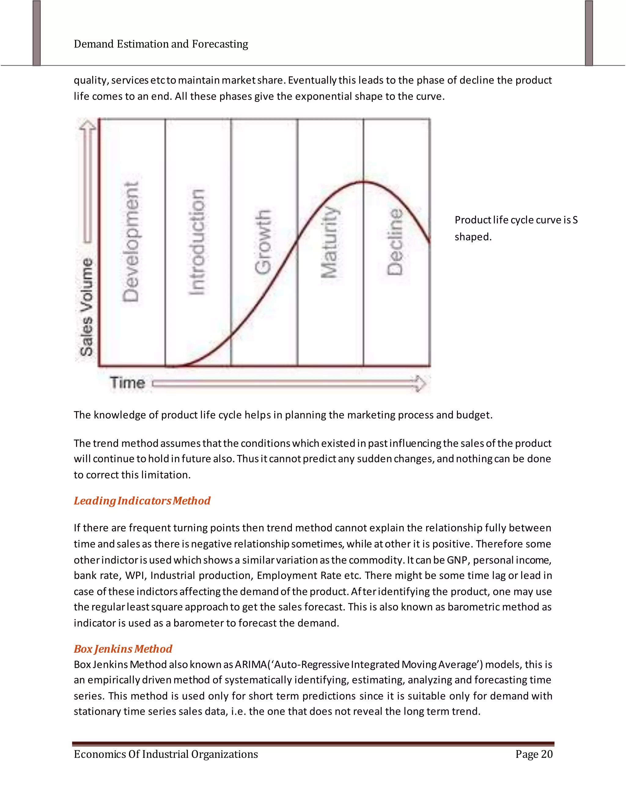
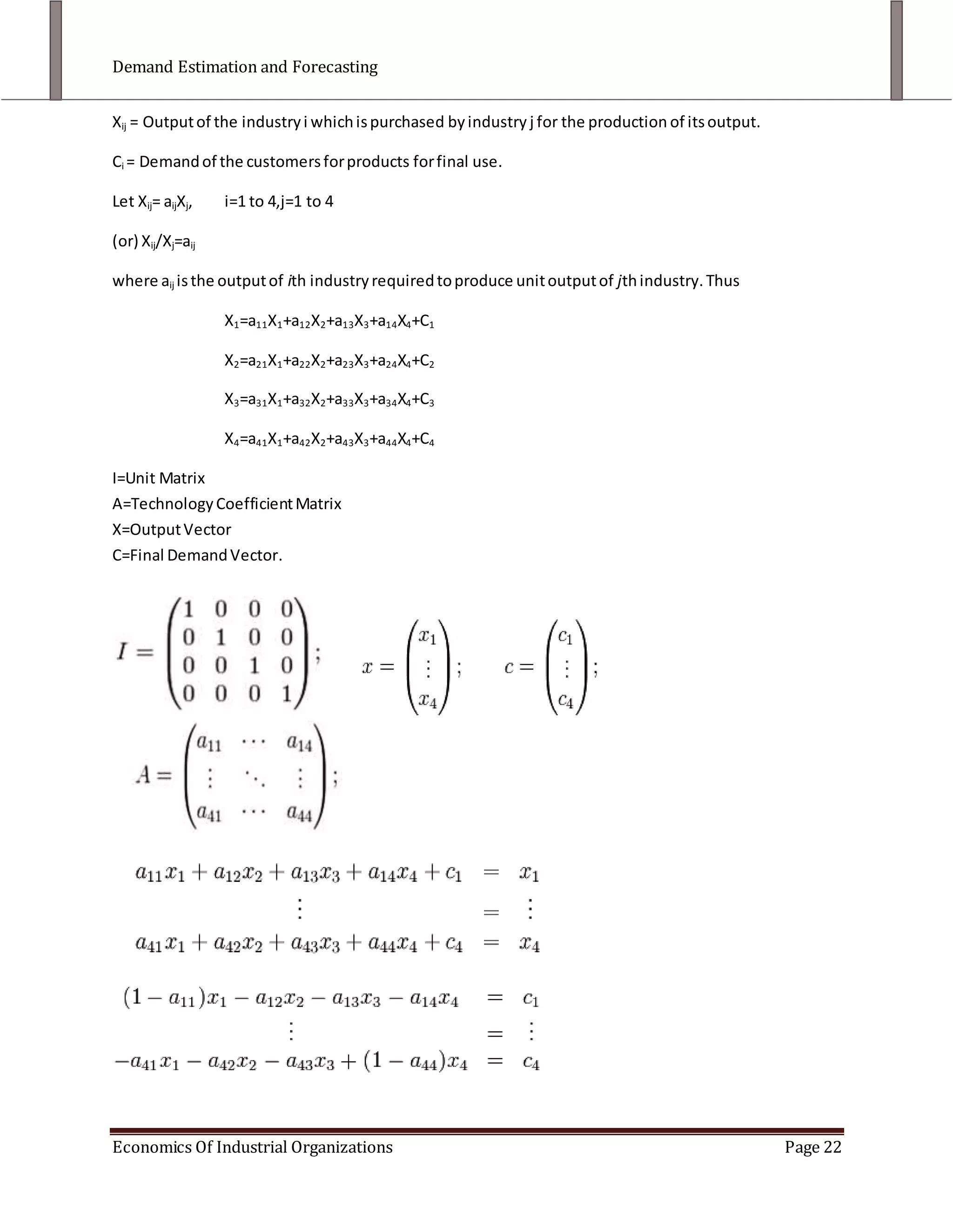
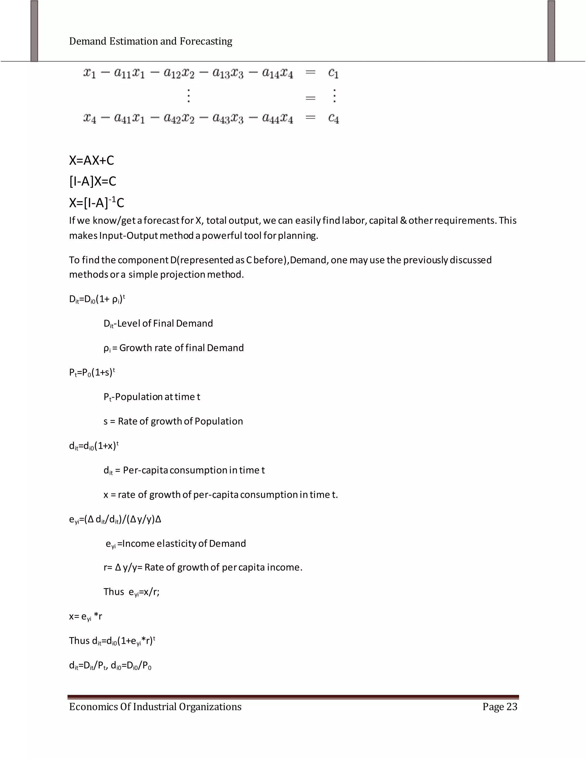
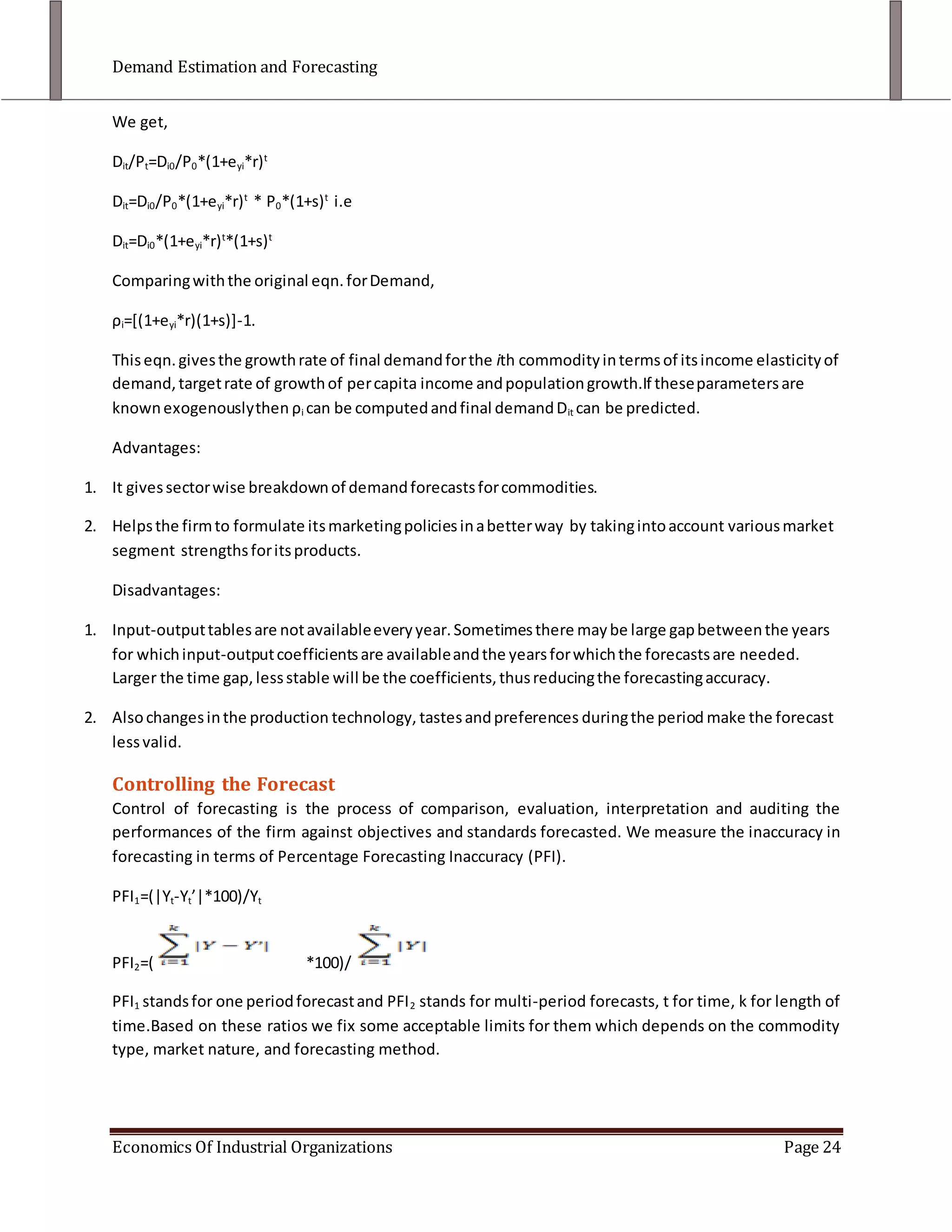
![Resource Needs Planning for HRM, Production, Financing, Marketing, etcType of Demand Forecasting<br />Based upon the time period for which demand forecasting is being done, it can either be short term or long term. Both are associated with the kind of business decisions that are required to be taken in order to meet the short term and long term changes in demand. A third type called medium term demand forecast can be done between the two. Short term demand forecast is usually done for periods of less than one year. <br />A short term demand forecast is done for production schedules of less than one year. It is done to deal with annual variations in sales. This takes care of an optimum use of current production capacity to meet the demand for the current financial year. Long term demand forecast are related to the need for capacity expansion or reduction depending upon the demand. It also takes care of changes in labor force needed and financial mechanism required to fund the expansion. This capacity expansion is usually not possible in the short run. If the firm anticipates major changes in demand then it will change the production capacity accordingly. For making a forecast a firm usually takes into account facts like population, competition in the market, technology, and government policies. The longer the time horizon of the forecast lesser is the accuracy of the forecast as the number of factors which can influence the demand becomes too high and their precise measurement is not possible. A medium term forecast is usually done to bridge the gap between the short term and long term forecast. It deals with business cycles that usually last for periods from two to five years. <br />The choice for the kind of forecast is also influenced by nature of the business. Where the output is diversified and it is easier to shift between different production mixes, short term forecast is preferred. In businesses with complex technology, like aircraft manufacturing, steel, motors where the shift in production mix is not easy and takes long time, long term forecast are done. The results of short term and the long term demand forecast may not be necessarily in agreement. The demand may be different for short term forecast and may show entirely different behavior for the long term forecast. <br />Approaches to Forecasting<br />Judgmental Approaches: the forecast is based upon the judgment and expertise of experts. <br />Experimental Approaches: A demand experiment is conducted among a small group of consumers who are adequately representative of characteristics of general population. This type of approach is adopted when the product being introduced is new, and there is no pre-existing data available. <br />Relational Causal Approaches: Interviews and other methods are used to determine the reasons why consumers purchase a particular product. Once these reasons are clear, the forecast can be done. <br />Time Series Approaches: Sales and other data for different markets, for different periods of time is analyzed to get a general trend or pattern in sales.<br />The Requirements for Demand Forecasting <br />For making a demand forecast of market firms have to do a market research in order to understand the probable future conditions of the markets thoroughly. Some of the elements of the market research are: <br />Consumer Related Elements: Total number of consumers, distribution of consumers/ products, total purchasing power and per capita household income, income elasticities, consumer tastes, social customs etc, consumer purchasing details, effect of design, color etc on consumer preferences. <br />Supplier Related Elements: Current level of sales, Current level of goods, Trends in sales and stocks, market share, patterns of seasonal fluctuations, Research and Development trends, company strength and weaknesses, product life cycle (age) and new product possibilities. <br />Market Related Elements: The effect of prices and price elasticities, product characteristics, identification of competitive and complementary products, number and nature of competitors, forms of market competition (price, advertisement, brand policy etc), general price levels, and prices of similar goods. <br />Other Elements: Economic environment of the country which includes levels of economic activities, employment, trends in income, national income, population, education etc, government policies, taxation and international economic climate. <br />The quantitative information related to these elements is collected and their effect on demand analyzed carefully. Then the firm may proceed to assess general economic and national situation in future (like population, income, price levels, technology, productivity, and international trade and government policies). Then the future total market demand for the commodity or product is estimated, based on the previously estimated general economic and national factors. In the last step the firm will estimate its share in the total market. <br />Factors affecting Method Selection<br />Time Factor: The lead time required for making decisions dependent on results of the model is crucial. Based on the time required for actually changing the output, in nature and level, it can be a short, medium or long term forecast. <br />Level of Forecasting: Demand forecasting may also be classified based upon whether it is done by an individual firm for its own product (micro), by an industrial or trade organization for the products of a particular industry (Industrial level) and if it is done for total industrial output based on national income or aggregate expenditure of that country.<br />General or Specific Forecasting: It can be general or total (if a firm has done a general forecast) or a specific forecast (if a firm has done area wise, commodity wise or industry wise forecast). <br />Problems and Methods of Forecasting: The methods and problems of forecasting demand for a new product (which has never been tested and there is no market data for it) are different from techniques used in forecasting for old product or commodity (for which market data and past behavior is available).<br />Classification of Goods: Demand forecast may depend upon the nature of goods like consumer and capital goods, durable and non-durables etc. <br />Knowledge of Different Market Conditions: Based upon the market structure and conditions (monopoly market, oligopolistic or competitive market) the forecast will be different. <br />Benefit Factors: The firms also have to do a cost-benefit analysis of the forecast method used. The expense and the effort invested should be justified by the potential benefits. The level of complexity and amount of accuracy required for forecast also effects the method selection. <br />Other Factors: Other special factors that need to be taken into account are political factors, sociological factors, psychology of consumers, and patterns of income distribution. <br />Techniques of Forecasting<br />The methods used may be divided broadly into two categories, qualitative and quantitative. Demand forecasting is full of uncertainties due to changing conditions. Consumer behavior is unpredictable as it is motivated and influenced by a multiplicity of forces. Every method developed for forecasting has its advantages and disadvantages and selection of the right method is crucial to make as accurate as possible forecast. A right combination of quantitative and qualitative methods is to be used.<br />Qualitative Techniques<br />Qualitative techniques are generally used when there is insufficient data available for quantitative analysis. They are also known as subjective methods as they are dependent upon intuition based on experience, intelligence, and judgment. They are also preferred for giving a quick estimate and cost savings. <br />Some of these techniques are as follows<br />Survey Method<br />The information about future demand of goods is obtained directly through a survey method. They are important for short term forecasts. Firms generally use them while introducing a new product into the market. It involves conducting consumer interviews, mailing questionnaires to consumers in order to judge their intentions about their demand for goods. Sometimes the employees, distributors and partners involved in the sales are interviewed. This is known as sales force composite method or collective opinion method. The salespersons are asked to report their estimates of expectations of sales in their territories. A similar exercise is done with the retailers and the wholesalers of the company. The average values thus obtained, from sales executives, marketing managers, business and managerial economists and other members of the trade, reflect the estimate of forecast.<br />Survey methods are dogged by numerous problems that are normally associated with surveys. There is always a risk of subjectivity, bias and over estimation or optimism about future (or a tendency to over report the expected sales), which may lead to a wrong forecast. The consumers picked for survey may not take the survey seriously or may not be a representative population sample. <br />Expert’s Opinion Method<br />This method is also known as the Delphi Method. Under this method a group of experts are repeatedly questioned for their opinion/comments on some issues and their agreements and disagreements are clearly identified. This involves a number of rounds involving their ‘interrogation, response and feedback’. In the first round they are asked for information necessary for forecast. The subsequent rounds involve questioning until a complete consensus is reached. The experts belong to a heterogeneous group with diverse background. This technique is used in technological forecasting, defense strategies, education and manpower planning, business demand forecasting etc. <br />This method has problems associated with selection of an appropriate expert panel, their timing schedules, time taken between different rounds and also the fact that the final result is not quantitative in nature. It is only a reasonable guess. <br />Consumer’s Interview Method<br />The consumers are contacted personally to know about their plans and preferences regarding the consumption of the product. All the potential buyers are then drawn and they are approached and asked how much they plan to buy the listed product in future. This method gives first hand information for demand forecast. There are three main methods for the interviews.<br />Complete Enumeration method: All the consumers of the product are interviewed and their future plans for product is ascertained. <br />Sample Survey Method: A sample of consumers is interviewed. <br />End use Method: Information about the end use of the product is collected form the industrial users to calculate the demand in industries, exports etc.<br />Historical Analogy Method<br />This method is used for forecasting demand for a new product or an existing product when introduced in a new area. When it is an existing product, then its sales data for a previous place (which has similar socio-economic conditions as the place where the product is being introduced) is taken for studying and estimating the future demand. In such cases one has to carefully account for sociological and psychological differences. Generally, places which are as similar as possible are taken for studying. If the product has not been used anywhere, then the past consumption pattern of some other similar product is taken as basis for forecasting the demand for the product. <br />The process is difficult as it is tough to find very similar locations, account for all the differences or find a similar product. <br />Test Marketing<br />It involves selecting a test area which can be regarded as true sample of total market. The product is launched in that area in the same manner in which it is intended to be used when product is launched nationally. All marketing devices are selected with this in mind. The sales data of the product tin the test area is then used to forecast the demand for the product nationally. <br />This method is costly and time consuming. Considerable energy and effort goes as all marketing devices are used for a small area. Selection of an appropriate test area is also difficult. The test needs to be run for a long period of time, to be sure about the sales data. Also differences in sociological and psychological characteristics need to be taken into account for this data. The launch if product in a test area gives competitors to prepare for the imitation of the product or prepare their own strategies to deal with the product. <br />Quantitative Techniques <br />Quantitative techniques are used for long run forecasting. They are used to explain time series and cross-section data for estimating long term demand. As they are quantitative in nature and give precise numbers, they are considered to be superior techniques of demand forecasting. Some of these methods are<br />Trend Method<br />The time series data of sales of a product may show some variation because of systematic forces. It may show a trend which is due to the effect of certain basic demand influencing factors like population, capital, technology etc. Cyclic variation in sales may be indicator of business cycles. There could be some variation based on seasonal variation also. Some other factors like strike, riots, theft, political disturbances etc will contribute to ‘random variation’. Time series analysis in statistics provides techniques by which all these variations and their effects on sales are isolated and identified. Several Quantitative techniques are used for this.<br />Graphical Method <br />Annual Sales data is plotted on paper and line is drawn through the points. This method is simple and less expensive.<br />Fitting Trend Equation<br />To get a relationship between sales of product and time, we have to fit the trend line by Least Square Method. The graph is plotted and trend line is plotted, which on extrapolation gives the forecasts for sale. The short term fluctuations are removed to get a more accurate forecast. This is ‘ironed out’ or ‘smoothened’ line. A three year moving average is used to remove the short term fluctuations in a more efficient manner. We may get the relationship in a form of an equation, each of which will tell us something unique about the sales relationship with time. If it is a <br />Linear Trend Equation: Demand for the product is increasing over time at a constant rate. <br />Quadratic Trend Equation: The marginal time increment of demand varies linearly with time, which means that total sales increases (or decreases) first and then decreases (or increases) thus showing a turning point on the sales-time graph. <br />Logarithmic Trend Equation: Time Elasticity of demand is constant. <br />Exponential Trend Equation: Rate of growth of demand is constant over time. <br />The advantage of this process is that it removes the short term fluctuations. Sales curve of any commodity eventually turns out to be ‘S’ shaped. This is known as product life cycle. The first stage is Research and Development, where product is market tested. No sales occur but a lot of expenditure is incurred. In Introduction stage product is launched and commercial exploitation and marketing begins. Sales grow in the next two stages of ‘market development’ and ‘exploitation’. Intensive advertising and sales promotion is done. At this optimum level of resource utilization the firm gets maximum profit here. As similar products by competitors flood the market, growth rate of sales decline in the ‘maturity’ stage. Price elasticity is very high, and in the later ‘saturation’ stage the high cross elasticity between different brands makes rate of sales growth zero. Marketing becomes ineffective, but firms maintain quality, services etc to maintain market share. Eventually this leads to the phase of decline the product life comes to an end. All these phases give the exponential shape to the curve. <br />Product life cycle curve is S shaped. <br />The knowledge of product life cycle helps in planning the marketing process and budget. <br />The trend method assumes that the conditions which existed in past influencing the sales of the product will continue to hold in future also. Thus it cannot predict any sudden changes, and nothing can be done to correct this limitation. <br />Leading Indicators Method<br />If there are frequent turning points then trend method cannot explain the relationship fully between time and sales as there is negative relationship sometimes, while at other it is positive. Therefore some other indictor is used which shows a similar variation as the commodity. It can be GNP, personal income, bank rate, WPI, Industrial production, Employment Rate etc. There might be some time lag or lead in case of these indictors affecting the demand of the product. After identifying the product, one may use the regular least square approach to get the sales forecast. This is also known as barometric method as indicator is used as a barometer to forecast the demand. <br />Box Jenkins Method<br />Box Jenkins Method also known as ARIMA(‘Auto-Regressive Integrated Moving Average’) models, this is an empirically driven method of systematically identifying, estimating, analyzing and forecasting time series. This method is used only for short term predictions since it is suitable only for demand with stationary time series sales data, i.e. the one that does not reveal the long term trend.The models are designated by the level of auto regression, integration and moving averages (P,d,q) where P is the order of regression, d is the order of integration and q is the order of moving average.<br />There are 3 components of the ARIMA process:<br />AR(Autoregressive) process.<br />MA(Moving Average) process.<br />Integration process.<br />AR process: Of order ‘p’, generates current observations as a weighted average of the past observations over p periods, together with a random disturbance in the current period.<br />Yt=μ+a1Yt-1+a2Yt-2+….+apYt-p+et<br />MA process: Order q, each observation of Yt is generated by the weighted average of random disturbances over the past q periods.<br />Yt= μ +et-c1et-1-c2et-2+….-cqet-q<br />Integrated Process: Ensures that the time series used in the analysis is stationary. The previous 2 equations are combined to form:<br />Yt=a1Yt-1+a2Yt-2+...+apYt-p+μ+et-c1et-1-c2et-2+…-cqet-q <br />Input-output model<br />An input-output model uses a matrix representation of a nation's (or a region's) economy to predict the effect of changes in one industry on others and by consumers, government, and foreign suppliers on the economy.One who wishes to do work with input-output systems must deal skillfully with industry classification, data estimation, and inverting very large, ill-conditioned matrices.Wassily Leontief, won the Nobel Memorial Prize in Economic Sciences for his development of this model in 1973. <br />Consider 4 industries,<br />Industry 1: X1=X11+X12+X13+X14+C1<br />Industry 2: X2=X21+X22+X23+X24+C2<br />Industry 3: X3=X31+X32+X33+X34+C3<br />Industry 4: X4=X41+X42+X43+X44+C4<br />Xij = Output of the industry i which is purchased by industry j for the production of its output.<br />Ci = Demand of the customers for products for final use. <br />Let Xij= aijXj, i=1 to 4,j=1 to 4<br />(or) Xij/Xj=aij <br />where aij is the output of ith industry required to produce unit output of jth industry. Thus<br />X1=a11X1+a12X2+a13X3+a14X4+C1<br />X2=a21X1+a22X2+a23X3+a24X4+C2<br />X3=a31X1+a32X2+a33X3+a34X4+C3<br />X4=a41X1+a42X2+a43X3+a44X4+C4<br />I=Unit Matrix <br />A=Technology Coefficient Matrix<br />X=Output Vector<br />C=Final Demand Vector.<br /> <br /> <br />X=AX+C<br />[I-A]X=C<br />X=[I-A]-1C<br />If we know/get a forecast for X, total output, we can easily find labor, capital & other requirements. This makes Input-Output method a powerful tool for planning.<br />To find the component D(represented as C before),Demand, one may use the previously discussed methods or a simple projection method.<br />Dit=Di0(1+ ρi)t<br />Dit-Level of Final Demand<br />ρi = Growth rate of final Demand <br />Pt=P0(1+s)t <br />Pt-Population at time t<br />s = Rate of growth of Population <br />dit=di0(1+x)t <br />dit = Per-capita consumption in time t<br />x = rate of growth of per-capita consumption in time t.<br />eyi=(∆ dit/dit)/(∆ y/y)∆ <br /> eyi =Income elasticity of Demand<br />r= ∆ y/y= Rate of growth of per capita income. <br />Thus eyi=x/r;<br />x= eyi *r<br />Thus dit=di0(1+eyi*r)t<br />dit=Dit/Pt, di0=Di0/P0<br />We get,<br />Dit/Pt=Di0/P0*(1+eyi*r)t<br />Dit=Di0/P0*(1+eyi*r)t * P0*(1+s)t i.e<br />Dit=Di0*(1+eyi*r)t*(1+s)t<br />Comparing with the original eqn. for Demand,<br />ρi=[(1+eyi*r)(1+s)]-1.<br />This eqn. gives the growth rate of final demand for the ith commodity in terms of its income elasticity of demand, target rate of growth of per capita income and population growth.If these parameters are known exogenously then ρi can be computed and final demand Dit can be predicted.<br />Advantages:<br />It gives sector wise breakdown of demand forecasts for commodities.<br />Helps the firm to formulate its marketing policies in a better way by taking into account various market segment strengths for its products. <br />Disadvantages:<br />Input-output tables are not available every year. Sometimes there may be large gap between the years for which input-output coefficients are available and the years for which the forecasts are needed. Larger the time gap, less stable will be the coefficients, thus reducing the forecasting accuracy.<br />Also changes in the production technology, tastes and preferences during the period make the forecast less valid. <br />Controlling the Forecast<br />Control of forecasting is the process of comparison, evaluation, interpretation and auditing the performances of the firm against objectives and standards forecasted. We measure the inaccuracy in forecasting in terms of Percentage Forecasting Inaccuracy (PFI).<br />PFI1=(|Yt-Yt’|*100)/Yt<br />PFI2=( *100)/ <br />PFI1 stands for one period forecast and PFI2 stands for multi-period forecasts, t for time, k for length of time.Based on these ratios we fix some acceptable limits for them which depends on the commodity type, market nature, and forecasting method. <br />REFERENCES/SOURCES:<br /> BIBLIOGRAPHY \l 1033 Armstrong, J. S. (2001). Standards and Practices for Forecasting. In Principles of Forecasting: A Handbook for Researchers and Practitioners (pp. 1-46). Kluwer Academic Publishers.<br />Barthwal, R. R. (2010). Industrial Economics An Introductory Textbook. New Age International Publishers.<br />J. Scott Armstrong, K. C. (2005). Demand Forecasting: Evidence-based Methods. In L. M. Southern, Strategic Marketing M.anagement: A Business Process Approach. <br />Savvides, D. S. (n.d.). Demand Estimation & Forecasting. EC611--Managerial Economics . Cyprus: European University Cyprus.<br />Webster, T. J. (2003). Managerial Economics Theory and Practice. San Diego: Academic Press.<br />Wilkinson, N. (2005). Managerial Economics A Problem Solving Approach. Cambridge: Cambridge University Press.<br />Mangerial Economics, Keat and Young<br />](https://image.slidesharecdn.com/demandestimationandforecasting-101120060005-phpapp01/75/Demand-estimation-and-forecasting-21-2048.jpg)

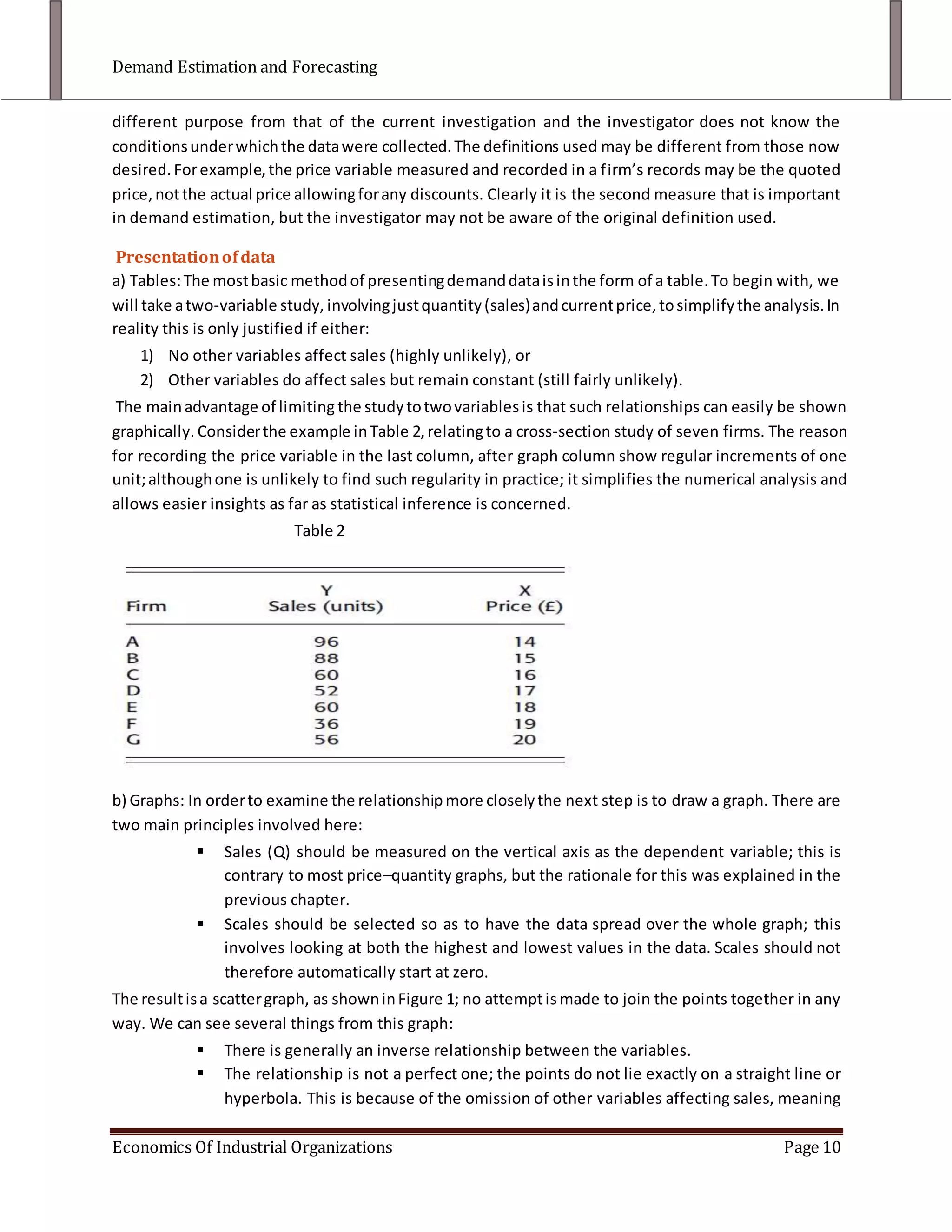
This document reviews demand estimation and forecasting methods in industrial organizations, detailing both qualitative and quantitative approaches. It outlines the process of demand estimation including model specification, data collection, and forecasting, while highlighting the importance of understanding market variables and their interrelationships. Additionally, it discusses various methodologies such as consumer surveys, market experiments, and statistical methods like regression analysis to estimate demand effectively.


