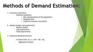
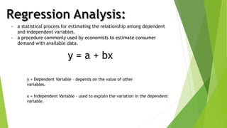
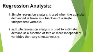
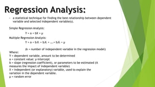
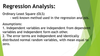
1. The document discusses demand estimation through regression analysis. Regression analysis uses empirical demand functions to estimate the relationship between a dependent variable (e.g. quantity demanded) and independent variables (e.g. price, income). 2. Simple and multiple regression analysis are explained. Simple regression uses one independent variable while multiple regression uses two or more. The Ordinary Least Squares method is commonly used to estimate coefficients. 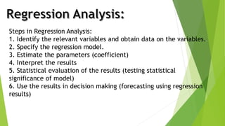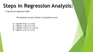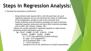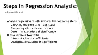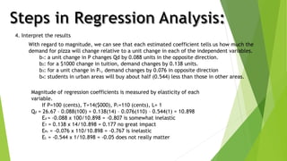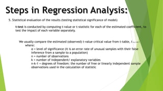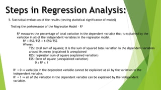3. The key steps in regression analysis are: specifying the model, estimating coefficients, interpreting results through statistical tests of significance, and using results for decision making like forecasting.

1. Reporter: Joone Elibert G. Eltanal
Program: MBA-I
Schedule: Block 1 Sat. 4:31-9:01
Professor: Judy Ann Ferrater-Gimena, DBA

2. - Define demand estimation
- Understand the methods of demand estimation
- Define and understand regression analysis

3. Demand Estimation is the process that involves
coming up with an estimate of the amount of
demand for a product or a service. It is confined to
particular period of time.

4. 1. Consumer interviews
- Potential problems:
• Not representative of the population
• Response bias
• Inability to answer accurately
2. Market studies and experiments
- Market studies
- Lab experiments
- Field experiments
3. Empirical demand functions
- In linear form, Q = a + bP + cM + dP᷊
- Regression analysis

5. - a statistical process for estimating the relationship among dependent
and independent variables.
- a procedure commonly used by economists to estimate consumer
demand with available data.
y = Dependent Variable – depends on the value of other
variables.
x = Independent Variable – used to explain the variation in the dependent
variable.
y = a + bx

6. 1.Simple regression analysis is used when the quantity
demanded is taken as a function of a single
independent variable.
2.Multiple regression analysis is used to estimate
demand as a function of two or more independent
variables that vary simultaneously.

7. - a statistical technique for finding the best relationship between dependent
variable and selected independent variable(s).
Simple Regression Analysis:
Y = a + bX + µ
Where:
Y = dependent variable, amount to be determined
a = constant value: y-intercept
b = slope (regression coefficient), or parameters to be estimated (it
measures the impact of independent variable)
X = independent (or explanatory) variable, used to explain the
variation in the dependent variable.
µ = random error
Multiple Regression Analysis:
Y = a + b1X1 + b2X2 + ….+ bkXk + µ
(k = number of independent variable in the regression model)

8. Ordinary Least Square (OLS)
- well-known method used in the regression analysis.
Assumptions:
1. Independent variables are independent from dependent
variables and independent form each other.
2. The error terms are independent and identically
distributed normal random variables, with mean equal to
zero.

9. Steps in Regression Analysis:
1. Identify the relevant variables and obtain data on the variables.
2. Specify the regression model.
3. Estimate the parameters (coefficient)
4. Interpret the results
5. Statistical evaluation of the results (testing statistical
significance of model)
6. Use the results in decision making (forecasting using regression
results)

10. 1. Identify the relevant variables and obtain data on the variables.
- Important variables are included in the regression analysis.
- The role of economic theory, the availability of data and other constraints help in
determining which variables to be included.
- main types of data used in regression
- cross sectional data
- time series
- pooled
2. Specify the regression model.
- For the purpose of illustration, let us assume that we have obtained cross-sectional data on
college students of 30 randomly selected college campuses during a particular month, with
the following equation: Qd = a + b1P + b2T + b3Pc + b4L + µ

11. 2. Specify the regression model.
Where:
Qd: Quantity demanded of pizza
P: average price of slice of pizza
T: annual tuition as proxy for income
Pc: price of cans of soft drinks
L: location of campuses
a: constant value or y-intercept
b: coefficient of independent variables to be estimated (slope)
µ: random error term standing for all other omitted variables
Qd = a + b1P + b2T + b3Pc + b4L + µ

12. 2. Specify the regression model.
The elasticity of each variable is calculated as usual:
Ed = dQ/dP x P/Q = b1 x P/Q
ET = dQ/dT x T/Q = b2 x T/Q
EPc = dQ/dPc x Pc/Q = b3 x Pc/Q
EL = dQ/dL x L/Q = b4 x L/Q

13. 3. Estimate the parameters (coefficient).
- Using ordinary least squares (OLS), with the particular set up of
regression equation we can now estimate the values of coefficients
of the independent variable as well as the intercept term.
- Usually statistical and econometrics packages are used to estimate
regression equation using excel and many other statistical packages
such as SPSS, SAS, EViews, LimDep, TSP…
- Results are usually reported in regression equation or table format,
containing certain information such as
Qd = 26.67 - 0.088P + 0.138T – 0.076 Pc – 0.544L
(0.018) (0.0087) (0.020) (0.884)
R² = 0.717 (the coefficient of determination)
R² (adj) = 0.67 (adjusted R²)
SE of Q estimate (SEE) = 1.64
F = 15.8 (F-Statistics)
Standard errors of the coefficient are listed in parentheses

14. 4. Interpret the results
Analyze regression results involves the following steps
Checking the signs and magnitudes
Computing elasticity coefficients
Determining statistical significance
It also involves two tasks
Interpretation of coefficients
Statistical evaluation of coefficients

15. 4. Interpret the results
Check signs of the coefficient according to economic theory and see
if they are as expected:
P: when price increases, Qd for Pizza decreases (negative sign)
T: Sign for proxy of income depends on whether pizza is a
normal or inferior good. (+,-)
Pc: expected sign for Pc is (-) because of complementary
relation (Pc increases, demand for pizza decreases)
L: Expected sign is (-) because in urban areas students have
varieties of restaurants (more substitutes), ⇒ they will
consume less pizza than their counterparts in other areas will.

16. 4. Interpret the results
With regard to magnitude, we can see that each estimated coefficient tells us how much the
demand for pizza will change relative to a unit change in each of the independent variables.
b1: a unit change in P changes Qd by 0.088 units in the opposite direction.
b2: for a $1000 change in tuition, demand changes by 0.138 units.
b3: for a unit change in Pc, demand changes by 0.076 in opposite direction
b4: students in urban areas will buy about half (0.544) less than those in other areas.
Magnitude of regression coefficients is measured by elasticity of each
variable.
If P=100 (cents), T=14($000), Pc=110 (cents), L= 1
Qd = 26.67 – 0.088(100) + 0.138(14) – 0.076(110) – 0.544(1) = 10.898
Ed = -0.088 x 100/10.898 = -0.807 is somewhat inelastic
ET = 0.138 x 14/10.898 = 0.177 no great impact
EPc = -0.076 x 110/10.898 = -0.767 is inelastic
EL = -0.544 x 1/10.898 = -0.05 does not really matter

17. 5. Statistical evaluation of the results (testing statistical significance of model)
t-test is conducted by computing t-value or t-statistic for each of the estimated coefficient, to
test the impact of each variable separately.
We usually compare the estimated (observed) t-value critical value from t-table, t α, n-k-1
where:
α = level of significance (it is an error rate of unusual samples with their false
inference from a sample to a population)
n = number of observations
k = number of independent/ explanatory variables
n-k-1 = degrees of freedom: the number of free or linearly independent sample
observations used in the calculation of statistic

18. 5. Statistical evaluation of the results (testing statistical significance of model)
t-test
To compare estimated t-value to critical t-value.
First: form the hypotheses
Second: Calculate t-value (observed t-value) of all independent variables
Third: Determine your level of significance (say 5%).
Fourth: Conclusion

19. 5. Statistical evaluation of the results (testing statistical significance of model)
t-test
First: form the hypotheses
Null hypothesis, H0: bi = 0
The null hypothesis means that there is no relationship between independent variable and
dependent variable. i.e. the variable in question has no effect on dependent variable when
other factors are held constant.
Alternative hypothesis, Ha: bi ≠ 0
The alternative hypothesis means that there is linear relationship between independent
variable and the dependent variable.
Since there are two hypotheses, rejecting one implies the other is automatically accepted (not
rejected)

20. 5. Statistical evaluation of the results (testing statistical significance of model)
t-test
Second: Calculate t-value (observed t-value) of all independent variables
In the pizza example:
tP = -0.088/0.018 = -4.89
tT = 0.138/0.087 = 1.58
tPc = -0.076/0.020 = -3.80
tL = -0.544/0.884 = -0.615

21. 5. Statistical evaluation of the results (testing statistical significance of model)
t-test
Third: Determine your level of significance (say 5%).
Using the rule of two, we can say that estimated coefficient is statistically significant (has an
impact on the dependent variable) if t-value is greater than or equal to 2.
In the pizza example above:
P & Pc are greater than 2 ⇒ statically significant ⇒the whole population has an effect on
demand.
T& L are Less than 2 ⇒ statistically insignificant ⇒the population as no effect on demand.
α = 0.05, n = 30, k= 4
t α, n-k-1 = t 0.05, 30-4-1 = t 05, 25 = 2.060

22. 5. Statistical evaluation of the results (testing statistical significance of model)
t-test
Compare absolute t-value with the critical t-value:
If absolute t-value > critical t-value, reject H0 and conclude that estimated coefficient is
statistically significant, otherwise accept H0.
var. t-value critical Decision Conclusion
P 4.889 > 2.060 reject significant
T 1.683 < 2.060 don’t reject not significant
Pc 3.800 > 2.060 reject significant
L 0.615 < 2.060 do not reject not significant

23. 5. Statistical evaluation of the results (testing statistical significance of model)
Testing the performance of the Regression Model – R²
R² measures the percentage of total variation in the dependent variable that is explained by the
variation in all of the independent variables in the regression model.
R² = RSS/TSS = 1-ESS/TSS
Where:
TSS: total sum of squares; it is the sum of squared total variation in the dependent variables
around its mean (explained & unexplained
RSS: regression sum of square (explained variation)
ESS: Error of square (unexplained variation)
0 ≤ R² ≤ 1
R² = 0 ⇒ variation in the dependent variable cannot be explained at all by the variation in the
independent variable.
R² = 1 ⇒ all of the variation in the dependent variable can be explained by the independent
variables

24. 5. Statistical evaluation of the results (testing statistical significance of model)
Testing the performance of the Regression Model – R²
In our example, R² = 0.717. This means that about 72% of the variation in the demand for pizza by college
students can be explained by the variation in the independent variables.

25. 5. Statistical evaluation of the results (testing statistical significance of model)
Adjusted R² (adjusted coefficient of determination)
In our example, adjusted R² = 0.67 which indicates that about 67% of the variation in Qd of pizza is
explained by the variations in the independent variables while 33% of these variations are unexplained
by the model.
Adjusted R² is calculated as
adjusted R² = R² - (k/(n-k-1))(1- R²)
adjusted R² = 0.72 – (4/25)(1-0.72) = .67

26. 5. Statistical evaluation of the results (testing statistical significance of model)
F-test
First: form the hypotheses
H0: All bi = 0 ( b1= b2 = b3 =…= bk = 0)
(k= number of independent variable in the regression model)
There is no relation between the dependent variable and independent variables. The
model cannot explain any of the variation in the dependent variable
Ha: at least one bi ≠ 0
A linear relation exists between dependent variable and at least one of the independent
variables.

27. 5. Statistical evaluation of the results (testing statistical significance of model)
F-test
Second: Calculate F-value
F = (explained variation/k) / (unexplained variation/n-k-1)
RSS = regression some of squares
ESS: error sum of squares
n: number of observation
k: number of explanatory variables
But F maybe re-written in term of R² as follows
In our example: F=15.8
The greater the value of F-statistics,
the more confident the researcher
would be that variables included in
the model have together a significant
effect on the dependent variable,
and the model has a high explanatory
power.

28. 5. Statistical evaluation of the results (testing statistical significance of model)
F-test
Third: Determine your level of significance (say 5%)
F α, k, n-k-1
α: level of significance
k: number of independent variables
n: number of observations or sample size
k, n-k-1: degrees of freedom
In our example: F.05, 4, 30-4-1 = F.05, 4, 25 = 2.76

29. 5. Statistical evaluation of the results (testing statistical significance of model)
F-test
Fourth: Compare F-value (observed F) with critical F-value
If F > Critical F value reject H0 and conclude that a linear relation exists between the
dependent variable and at least one of the independent variable F= 15.8 > F.05, 4, 25 = 2.76
6. Use the results in decision making (forecasting using regression results).
- Future values of demand can easily be predicted or forecasted by plugging values of independent
variables in the demand equation.
- Only we have to be confident at a given level that the true Y is close to the estimated Y.
- Since we do not know the true Y, we can only say that it lies between a given confidence interval.
- The interval is Ŷ± t α, n-k-1 X SEE
- Confidence interval tells that we are, say, 95% confident that the predicted value of Qd lies
approximately between the two limits.