The document discusses deadweight loss that occurs due to taxes and monopolies. It provides the following key points:
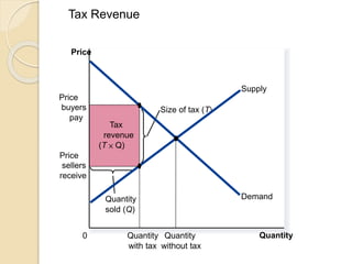
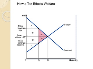
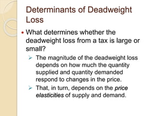
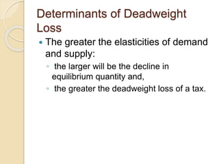
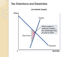
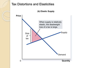
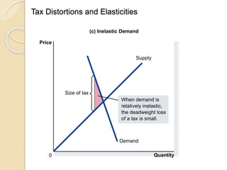
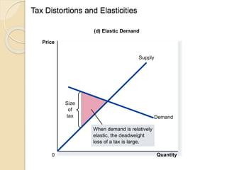
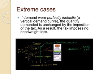
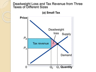
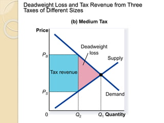
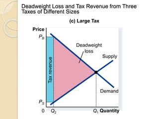
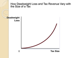
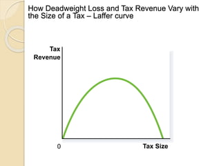
- A tax creates a wedge between the price paid by buyers and received by sellers, resulting in a reduction in quantity traded and deadweight loss for society. The size of the deadweight loss depends on the price elasticities of supply and demand.
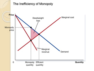
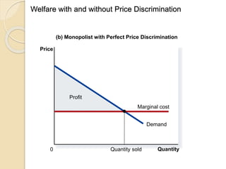
- Monopolies also create deadweight loss by setting price above marginal cost. Price discrimination allows monopolies to reduce deadweight loss by charging different prices to different customers.
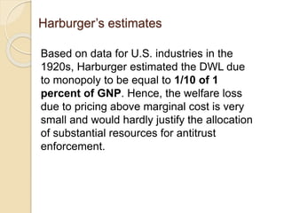
- Estimating deadweight loss is difficult but important for evaluating market efficiency. Two approaches discussed are Harburger's method using industry profit margins and Cowling and Mueller's method


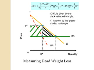
![Harburger’s Approach
The ABH dead weight triangle is approximated by the
following equation (equation 4.1 in the text):
))((
2
1
MCCM QQPPDWL
By algebraic manipulation it can be shown that:
**
2
1 2
QPdDWL [1]](https://image.slidesharecdn.com/deadweightloss-160220182149/85/Dead-weight-loss-33-320.jpg)


![To estimate industry-level price elasticities (),
Cowling and Mueller took advantage of the fact
that the firm’s profit maximizing price (P*)
satisfies the following condition:
MCP
P
*
* [2]
Recall that d is the price-cost margin . Thus we can
say:
MCP
P
d
*
*1
[3]
Thus by equation [2], we can say:
d
1 Thus if you can
estimate d, you
can estimate ](https://image.slidesharecdn.com/deadweightloss-160220182149/85/Dead-weight-loss-37-320.jpg)
![Thus substitute 1/d for in equation [1] and you
get:
**
2
1
**
1
2
1 2
QdPQPd
d
DWL
[4]
Substituting (P*- MC)/P* for d in equation [4] gives us:
*
2
1
*)*(
2
1
**
*
2
1
QMCPQP
P
MCP
DWL [5]
Thus, Cowling and Mueller showed that DWL for an
industry was equal to ½ of the economic profits () of
firms in the industry.](https://image.slidesharecdn.com/deadweightloss-160220182149/85/Dead-weight-loss-38-320.jpg)


![Interdependence of nations[1]](https://cdn.slidesharecdn.com/ss_thumbnails/interdependenceofnations1-111214194721-phpapp02-thumbnail.jpg?width=640&height=640&fit=bounds)


