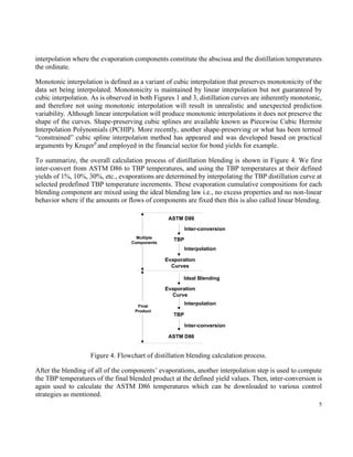
The document discusses a new technique for optimizing distillation blending and cutpoints in oil refineries to improve efficiency and control over product quality and yield. It involves manipulating true boiling point (TBP) curves by adjusting initial and final boiling points in order to optimize blending recipes and meet product specifications. The proposed method employs monotonic interpolation to replace traditional splines for enhanced accuracy in distillation temperature calculations, ultimately aiding in the production of ultra-low sulfur fuels.

1. 1
DISTILLATION BLENDING AND CUTPOINT TEMPERATURE
OPTIMIZATION IN SCHEDULING OPERATIONS
Brenno C. Menezes, Center for Information, Automation and Mobility, Technological Research Institute, São Paulo, SP, Brazil
Jeffrey D. Kelly, Industrial Algorithms, Toronto, ON, Canada
Ignacio E. Grossmann, Chemical Engineering Department, Carnegie Mellon University, Pittsburgh, PA, United States
Lincoln F.L. Moro, REVAP Refinery, PETROBRAS, São José dos Campos, SP, Brazil
Keywords: Cutpoint optimization, Distillation curve, Fuel production, Distillation and blending integration
Introduction
In oil refinery manufacturing, final products such as fuels, lubricants and petrochemicals are produced
from crude-oil in process units considering their operations in coordination with tanks, pipelines,
blenders, etc. In this process, the full range of hydrocarbon components (crude-oil) is transformed
(separated, reacted, blended) into smaller boiling-point temperature ranges resulting in intermediate and
final products, in which planning, scheduling and real-time optimization using distillation curves of the
streams can be used to effectively model the unit-operations and predict yields and properties of their
outlet streams.1
The hydrocarbon streams’ characterization or assays of both the crude-oil and its
derivatives are decomposed, partitioned or characterized into several temperature cuts based on what are
known as True Boiling Point (TBP) temperature distribution or distillation curves.2,3
These are one-
dimensional representations of how quantity (yields) and quality (properties) data of hydrocarbon
streams are distributed or profiled over its TBP temperatures where each cut is also referred to as a
component, pseudocomponent or hypothetical in process simulation and optimization technology.4
To improve efficiency, effectiveness and economy of mixing/blending, reacting/converting and
separating/fractionating inside the oil-refinery, we proposed a new technique to optimize the blending
of several streams’ distillation curves with also shifting or adjusting cutpoint temperatures of distilled
streams, i.e, their initial boiling point (IBP) and final boiling point (FBP), in order to manipulate their
TBP curves in either off-line or on-line environment. By shifting or adjusting the front-end and back-
end of the TBP curve for one or more distillate blending streams, it allows for improved control and
optimization of the final product demand quantity and quality, affording better maneuvering closer and
around downstream bottlenecks such as tight property specifications and volatile demand flow and
timing constrictions. This shifting or adjusting of the TBP curve’s IBP and FBP (front- and back-end
respectively) ultimately requires that the unit-operation has sufficient handles or controls to allow this
type of cutpoint variation where the solution from this higher-level optimization would provide set points
or targets to a lower-level advanced process control systems, which are now commonplace in oil
refineries.
The unit-operation processing and product blending are integrated in this novel technique using
monotonic interpolation to blend and cut distillation temperatures and evaporations for petroleum
products in an optimization environment. Blending distillation temperatures is well known in simulation

2. 2
whereby cumulative evaporations at specific temperatures are mixed together then these data points are
used in piece-wise cubic spline interpolations to revert back to the distillation temperatures. Our method
replaces the splines with monotonic splines to eliminate Runge's phenomenon (overshooting) and to
allow the distillation curve itself to be adjusted by optimizing its initial and final boiling points (IBP and
FBP) known as cutpoints. By optimizing both the recipes of the blended material and its blending
component distillation curves, very significant benefits can be achieved especially given the global push
towards ultralow sulfur fuels (ULSF) due to the increase in natural gas plays reducing the demand for
other oil distillates. One example is provided to highlight and demonstrate the technique.
Distillation Curve Overview
Hydrocarbon streams (crude-oils, fuels, petrochemicals) are characterized by distillation curves in terms
of their quantity (yield) and quality (properties) and how they vary with respect to temperature. These
data are determined by experimental methods using small-scale laboratory distillation columns in which
hydrocarbon fractions are collected at certain boiling-point temperatures to define their quantity and
quality data or assay at each boiling temperature. These data can then be used in mathematical models,
either in rigorous engineering or simplified empirical simulation and optimization environments, to
determine the yields and properties of distillation, separation or fractionation unit-operation outputs.3
Integrated with this can be the final product recipes necessary to match demand quantity and quality
specifications such as specific gravity, sulfur, pour-point and evaporation temperatures of the fuels so
that simultaneous distillation blending and cutpoint temperature shifting or adjusting can be simulated
and optimized together as is proposed in this paper.
Since obtaining TBP curve data directly from a laboratory distillation run is expensive and time-
consuming, the normal procedure for the distilled products is to determine distillation curves by applying
American Society for Testing and Material (ASTM) methods such as D86 (atmospheric) and D1160
(vacuum) or simulated distillation (SD) methods, which uses gas chromatography (GC) such as D2887
and D7169. These experiments are based on reduced numbers of separation stages and can fortunately
be easily interconverted to TBP data with sufficient accuracy and precision.2
Figure 1 shows both the
ASTM D86 and TBP data from the Colorado School of Mines (2012) for a straight-run gasoline stream
from a crude-oil distillation unit (CDU), plotted with volume yield percent as the ordinate and
temperature as the abscissa.
A well-known observation, with regard to Figure 1, is that the ASTM D86 and TBP temperatures are
near equal at their 50% yield point, whereas D86 yields are underestimated below the 50% yield and
D86 yields are overestimated above the 50% yield. Riazi correlations used to convert ASTM D86 (D01
to D99) to TBP (T01 to T99) temperatures at conventional yield percentages of 1%, 10%, 30%, 50%,
70%, 90%, and 99%, where the same equations can be simply inverted in order to convert from TBP to
ASTM D86 can be found in Colorado of Mines reference.5

3. 3
Figure 1. ASTM D86 and TBP volume yield percent curves.
Note that for the IBP and FBP we use the percent evaporated at 1% and 99% instead of 0% and 100%,
and this is a well-known recommendation found in several sources. Other interconversion correlations
can be found in Riazi and Daubert6
and Daubert.7
Also note that for temperatures greater than ca. 650
degrees F and at atmospheric pressure, thermal cracking may occur due to pyrolysis reactions. In these
situations, ASTM D1160 should be use, which is conducted at a lower pressure (near vacuum), where
its temperatures need to be corrected back to atmospheric pressure.
For product streams separated from unit-operations such as distillation columns and fractionation towers,
the experimental TBP and/or ASTM distillation curves reflect the non-ideal separation inside the vessels
as seen in Figure 2, where increments in the temperature (abscissa) cause a non-linear increment in the
evaporations (ordinate). For example, if we compare a CDU’s crude-oil feed distillation curve with all
of its product distillation curves as shown in Figure 3, it is interesting to see what are known as overlaps
between the light and heavy adjacent products; this represents what is referred to as non-sharp or non-
ideal fractionation.8
Figure 2. Non-linear behavior in the extremes of the distillation curves.

4. 4
Figure 3. Feed and product yield curves in a crude distillation unit (CDU).
Distillation Blending Using Monotonic Interpolation
The difficulty with blending the distillation temperatures from several component materials is that these
TBP distillation temperatures do not blend linearly on a mass or volume basis. Although there is some
use of what are commonly referred to as blending indices or property transforms for distillation
temperatures (and used effectively for other properties such as cloud-point, pour-point, viscosity, etc.)
which then allow the indexed or transformed properties to be blended linearly, literature on their
mathematical structure and coefficients is scarce. Instead, an acceptable approach is to convert the TBP
temperatures to evaporation cumulative compositions at several pre-defined temperatures using
monotonic interpolation of which linear interpolation is inherently monotonic but may not be as accurate
as higher-order monotonic interpolations. Unfortunately if non-monotonic interpolation is used such as
cubic splines, then oscillating behavior around the breakpoints will occur and is well known as Runge’s
phenomenon (overshooting). The temperature range should be defined to span all of the expected TBP
temperatures for all of the distillates included in the blend at a suitable level of resolution or temperature
discretization. After the set of evaporation components have been blended together using the recipes
fractions of each component blended, the blended product’s distillation temperatures at 1%, 10%, 30%,
50%, 70%, 90% and 99% evaporated, distilled or yielded are computed by again using monotonic

5. 5
interpolation where the evaporation components constitute the abscissa and the distillation temperatures
the ordinate.
Monotonic interpolation is defined as a variant of cubic interpolation that preserves monotonicity of the
data set being interpolated. Monotonicity is maintained by linear interpolation but not guaranteed by
cubic interpolation. As is observed in both Figures 1 and 3, distillation curves are inherently monotonic,
and therefore not using monotonic interpolation will result in unrealistic and unexpected prediction
variability. Although linear interpolation will produce monotonic interpolations it does not preserve the
shape of the curves. Shape-preserving cubic splines are available known as Piecewise Cubic Hermite
Interpolation Polynomials (PCHIP). More recently, another shape-preserving or what has been termed
“constrained” cubic spline interpolation method has appeared and was developed based on practical
arguments by Kruger9
and employed in the financial sector for bond yields for example.
To summarize, the overall calculation process of distillation blending is shown in Figure 4. We first
inter-convert from ASTM D86 to TBP temperatures, and using the TBP temperatures at their defined
yields of 1%, 10%, 30%, etc., evaporations are determined by interpolating the TBP distillation curve at
selected predefined TBP temperature increments. These evaporation cumulative compositions for each
blending component are mixed using the ideal blending law i.e., no excess properties and no non-linear
behavior where if the amounts or flows of components are fixed then this is also called linear blending.
Figure 4. Flowchart of distillation blending calculation process.
After the blending of all of the components’ evaporations, another interpolation step is used to compute
the TBP temperatures of the final blended product at the defined yield values. Then, inter-conversion is
again used to calculate the ASTM D86 temperatures which can be downloaded to various control
strategies as mentioned.
ASTM D86
TBP
Inter-conversion
Evaporation
Curves
Interpolation
Ideal Blending
Evaporation
Curve
Multiple
Components
Final
Product
ASTM D86
Interpolation
Inter-conversion
TBP

6. 6
Cutpoint Temperature Optimization (CTO)
Distillation curves of petroleum products are typically plotted as TBP temperature versus relative yield
percent, where we have chosen to represent the curves in the opposite way, indicating that the TBP
temperature is now our independent variable or degree-of-freedom in the optimization. When yields,
evaporations or relative amounts distilled of the distillates are used as a function of temperature, the IBP
(T01) and FBP (T99) can be manipulated for example to adjust or shift the distillation curve by
interpolation and/or extrapolation in order to increase or decrease the front-end and back-end of the
curves, as graphically depicted in Figure 5. The incremental or marginal adjustment or shifting can also
be likened to fine-tuning the distillation curve, and this will ultimately translate to changing all of the
relative yield values along the total or overall TBP temperature range of the distillate stream. This will
have the desired effect that we can alter the evaporation amounts in the downstream blending to better
control and optimize the blend quantity and quality specifications to meet market demands. However,
when we manipulate the T01 and/or T99 for any distillate component stream, these values
(interconverted to D01 and D99 if required) must be sent down as targets or setpoints to an appropriate
advanced process control strategy on the respective upstream unit-operation such as an atmospheric
crude-oil distillation column or the main fractionator tower of a fluidized bed catalytic cracking unit
(FCCU). Fortunately, such strategies are available whereby reliable online analyzers measure in real-
time or near-time (including sampling and analysis delays) ASTM D86 temperatures, which can be
linked to pump-around heat exchanger duty and draw tray temperature controls to achieve the desired
increase and/or decrease in initial and final cutpoint temperatures.
Figure 5. Distillation curve adjustment or shifting, as a function of TBP temperature.

7. 7
To manipulate distillation curves based on the cutpoint optimization proposed, process engineers need
to bear in mind that cutpoint temperatures (IBP and FBP) are strong functions of both the light and heavy
draw flows and temperatures for the distillates leaving the column, tower or side-strippers. Other causal
factors or process variables affecting cutpoint temperatures include draw tray technology, location,
efficiency and pressure, pump-around flows (intermediate refluxes), duty and return temperature as well
as stripping steam flow which all influence and contribute to the column’s internal vapor and liquid
traffic defining its separation/fractionation operation. For Nelson (1945)11
there are four principles to
manage the production of distillates. First, the yield of a given product or fraction is primarily a function
of the composition of the feed mixture, not the degree of separation. Second, the number of trays only
slightly alters the boiling range of the products as defined by ASTM initial and final boiling points.
Third, the initial boiling point of side draw products is always low, and must be corrected by either steam
stripping or reprocessing (refluxing). Forth, the final boiling point of a side draw product is primarily
controlled by opening or closing the draw valve to change the yield.
So, based on these principals regarding the cutpoint manipulation, we introduce the cutpoint temperature
optimization method, where the complete formulation is found in Kelly et al.4
Our new distillation curve
adjustment or shifting technique to perform temperature cutpoint optimization is straightforward to
implement mathematically. The concept is to assume that a typical distillation curve can be reasonably
decomposed or partitioned into three distinct regions or parts i.e., a front-end, middle and back-end. The
different sections can be sufficiently approximated as straight-lines or piece-wise continuous from OT01
to OT10 for the front-end, OT10 to OT90 for the middle and OT90 to OT99 for the back-end where “O”
stands for “old” and of course “N” stands for “new” for the new adjusted or shifted 1% and 99%
temperatures, found in eqs 1 and 2 i.e., NT01 and NT99.
Eqs 1a and 1b model both the yield (YNT01) and the change or difference in the yield (DYNTO1) when
we adjust or shift T01 from OT01 to NT01 assuming a constant slope determined from the unadjusted
or unshifted old or original curve. Obviously if NT01 = OT01 (no change) then YNT01 = 0.01 and
DYNT01 = 0.0 as expected.
YNT01 = 0.10 −
0.10 − 0.01
OT10 − OT01
(OT10 − NT01) (1a)
DYNT01 = 0.10 − YNT01 (1b)
Similarly, for the back-end regime we can model the new yield at NT99 and its delta yield DYNT99 in
eqs 2a and 2b, respectively. And, if NT99 = OT99 then YNT99 = 0.99 and DYNT99 = 0.0, trivially.
YNT99 = 0.90 +
0.99 − 0.90
OT99 − OT90
(NT99 − OT90) (2a)
DYNT99 = YNT99 − 0.99 (2b)

8. 8
Eq 3 easily models the increase or decrease in the new flow from the upstream unit-operation depending
on the amount of adjustment or shifting of the cutpoint temperature variables NT01 and NT99 where OF
is the old or measured flow value.
NF = OF(1 + DYNT01 + DYNT99) (3)
A useful feature of adjusting or shifting the distillation curve, along the original front and back-end
slopes, is its ability to predict the marginal increase or decrease in the distillate stream flow directly
without having to resort to a separate equation with unknown coefficients that will need to be
continuously calibrated.
Given that our TBP distillation curve plots relative yield versus temperature, we need to normalize each
new yield found in eq 4 which correspond to the temperatures NT01, OT10, OT30, OT50, OT70, OT90
and NT99. Again, if both DYNT01 = DYNT99 = 0.0 because NT01 = OT01 and NT99 = OT99 then we
are obviously left with our old or original TBP distillation curve for the upstream unit-operation
component distillate stream yield profile.
NY01 =
0.01
(1 + DYNT99)
(4a)
NY10 =
0.10 + DYNT01
(1 + DYNT01 + DYNT99)
(4b)
NY30 =
0.30 + DYNT01
(1 + DYNT01 + DYNT99)
(4c)
NY50 =
0.50 + DYNT01
(1 + DYNT01 + DYNT99)
(4c)
NY70 =
0.70 + DYNT01
(1 + DYNT01 + DYNT99)
(4d)
NY90 =
0.90 + DYNT01
(1 + DYNT01 + DYNT99)
(4e)
NY99 =
0.99 + DYNT01
(1 + DYNT01)
(4f)
The idea for these equations is straightforward, in the sense that if we increase or decrease the front-end
and back-end, then given their delta yield amounts found in eqs 1b and 2b we can easily adjust the new
yields given the old yields, where the old yields are, of course, the well-defined 1%, 10%, 30%, etc.
values. However, it is re-emphasized that our approach is to incrementally or marginally shift or adjust

9. 9
the NT01 and NT99 so as not to significantly disrupt the adjacent distillation streams, and can be
controlled by specifying acceptable bounds on NT01 and NT99 in the optimization.
Considering that the example shown in Figure 5 is a straight-run gasoline, its old IBP (OT01) and FBP
(OT99) are 91 and 230 o
F as seen in Figure 6. If in an optimization problem the new IBP (NT01) and
FBP (NT99) change to 85 and 214 o
F, respectively, we expect a hydrocarbon amount increase in the
front-end (lighter fraction) and decrease in the back-end (heavier fraction) of the distillation curve. By
using eqs 1 and 2, the new yields are YNT01 = -1.45% e YNT99 = 95.87%, which means the front-end
of the gasoline in the optimized problem receives heavier hydrocarbon fractions from its lighter adjacent
neighbor and the back-end is reduced giving material to its heavier adjacent neighbor, both with respect
to the extrapolation in the initial (front-end) and final (back-end) of the distillation curve. Finally, to
renormalize the curve, the yield deviations are calculated, giving DYNT01= 2.45% and DYNT99 = -
3.13%, and then a new distillation curve considering eq 4 to update the evaporations is plotted ( ).
The renormalization procedure is due to the relative value of the evaporations with respect to gained or
lost amounts of yields in the IBP and FBP extremes.
Figure 6. Distillation curve renormalization after the new IBP (NT01) and FBP (NT99).
Also, it should be pointed out that our use of the term cutpoint is somewhat different than is found, for
example in the work of Zhang et al.,11
Li et al.,8
Alattas et al.12
and Menezes et al.,3
in which a cutpoint
is defined as the lower/initial and upper/final temperatures on the TBP of the entire crude oil, which
hypothetically represents the crude-oil fraction distilled or evaporated from the distillation tower such
as a CDU. Instead given that the TBP curve of a CDU’s crude-oil mixture is not normally available in

10. 10
practice, and especially if the feed is to an FCCU main fractionator, which is rarely known, we use the
definition commonly found in oil-refinery operations of defining cutpoint temperatures as the smallest
and/or largest controllable separation or fractionation temperature (i.e., IBP, 5% or 10% and 90%, 95%
or FBP) between adjacent cuts, fractions or streams from a distillation tower. Other approaches as those
found in Mahalec and Sanchez13
use assay and CDU operations data to apply hybrid models, where
partial least squares (PLS) models involving operating variables to predict product distillation curves
define vertical deviation between front- and back-sections of the curves to the straight line in the middle
section.
Example: Diesel Blending and Cutpoint Temperature Optimization
This case is taken, in part, from Erwin15
in terms of using his ASTM D86 (1 atm) temperatures for his
four experimental diesel components (DC1 to DC4), as shown in Table 1 and Figure 7, where the dotted
line represents the final product blend distillation curve.
Table 1. Example 2's InterConverted TBP (ASTM D86) Temperatures in Degrees F.
Our blending and cutpoint temperature optimization objective function is to maximize the flow of DC1
and DC2, subject to their relative and arbitrary pricing of 0.9 for DC1 and 1.0 DC2, with lower and upper
bounds of 0.0 and 100.0 each. For simplicity, we have fixed each of the flows for DC3 and DC4 to a
marginal and arbitrary value of 1.0, and the total blend flow cannot exceed 100.0. The typical ASTM
D86 temperature specification for international diesel sales is D10 ≤ 480, 540 ≤ D90 ≤ 640, and D99 ≤
690 degrees F. To make this problem more interesting, we have set the bounds to D10 ≤ 470, 540 ≤ D90
≤ 630 and D99 ≤ 680. This ensures that it is not possible to satisfy the diesel blend with the most valuable
DC2 component as its D10, D90, and D99 temperatures are all greater than our blended diesel's
distillation temperature specification. Furthermore, it is also not possible to fill the blend with all DC1,
because its D90 does not comply with the specification. As such, this forces a mixture of DC1 and DC2
and as we shall see, this also requires an adjustment or shifting to the distillation curve for DC1 where
only the DC1 material is allowed to have manipulated cutpoint temperatures. At the optimized solution
NT01 = 312.8 and NT99 = 689.3, which are both different than their original values of OT01 = 305.2
and OT99 = 715.7. Since both their frontend and backend temperatures have been reduced we expect
DC1 DC2 DC3 DC4
1% 305.2 (353) 322.2 (367) 327.0 (385) 302.4 (368)
10% 432.9 (466) 447.1 (476) 405.2 (435) 369.7 (407)
30% 521.6 (523) 507.1 (509) 457.1 (462) 441.0 (449)
50% 565.3 (551) 549.5 (536) 503.3 (492) 513.8 (502)
70% 606.4 (581) 598.4 (573) 551.1 (528) 574.3 (550)
90% 668.3 (635) 666.1 (634) 605.8 (574) 625.4 (592)
99% 715.7 (672) 757.7 (689) 647.0 (608) 655.2 (620)

11. 11
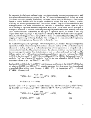
that the new flow for DC1 is less than the old flow and it is NF = 37.06 and OF = 39.24; consequently,
the flow for DC2 is 60.94, which is consistent with the total flow of 100.0. The new and optimized TBP
curve for DC1 given its front- and back-end shifts is now [(1.053%,312.8), (10.015%,432.9),
(31.188%,521.6), (52.361%,565.3), (73.534%,606.4), (94.707%,668.3), (98.995%,689.3)], where the
new yields are computed.
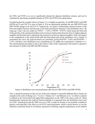
Figure 7. Example’s TBP distillation curves, including the final blend.
Distillation Blending and Cutpoint Temperature Optimization (DBCTO) in
Scheduling Operations
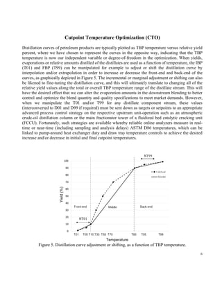
The cutpoint temperature optimization (CTO) is a conservative and adaptive TBP cutpoint method
to marginally/incrementally adjust/shift distillate yields when “non-sharp” (non-ideal, imperfect)
separation exists i.e., without an “infinite” number of stages and/or reflux. It uses ASTM D86
cutpoint temperatures or simulated distillation that are not as suitable as TBP temperatures given that
they over-predict the initial boiling-point (IBP) and under-predict the final boiling-point (FBP), but
these experimental methods are quicker to measure in the lab and field.
To apply the CTO method in the final fuel blending, we use the distillation curves of the distilled
streams from units such as CDU and FCCU to integrate their operation to variations in quantity and
quality of the produced intermediate fuels in order to fulfill final fuel demands in blendshops. Figure

12. 12
8 shows the crude-oil and fuel management systems, where the distillation blending and cutpoint
temperature optimization (DBCTO) is seen in between the crude-to-fuel transformations and the fuel
blending and distribution. The proposed technique opens an avenue in the search for applications
and opportunities on smart process operations in fuels industries.15
Figure 8. Crude-oil and fuel management systems.16
Conclusions
In this paper, we have presented the fine points of performing distillate blending and cutpoint
temperature optimization using monotonic interpolation. The first step of the procedure is to convert
from faster and less-expensive experimental methods, such as ASTM D86, to the slower and more
expensive TBP temperatures, using well-established interconversion analytical expressions. These
interconverted TBP temperatures are converted to cumulative evaporations similar to pseudo-
components in process design simulators using monotonic interpolation, blended linearly by mass or
volume, then converted back to TBP temperatures using another monotonic interpolation. If required,
these values are interconverted back to ASTM D86, and this defines the second step. The third step is to
adjust or shift the front-end and/or back-end of one or more of the component TBP distillation curves by
optimizing the T01 (1%) and/or T99 (99%) cutpoint temperatures, while respecting the relative yields
of the adjusted or shifted distillation curves. It is the third step that, to our knowledge, has not been
discussed in the literature prior to this work and if distillation blending indices are used instead of mixing,
cutting, and interpolating with evaporation components then this type of temperature cutpoint
optimization is not possible. As highlighted in the Introduction, significant economic benefits can be
achieved by implementing such an algorithm, especially for ultralow sulfur fuels which always require
accurate prediction of key evaporation points on the final product distillation curves.

13. 13
References
1. Kelly, J.D., “Formulating Production Planning Models”. Chemical Engineering Progress, 2004,
100, pages 43-50.
2. Riazi, M.R., “Characterization and Properties of Petroleum Fractions. American Society for
Testing and Materials”, 2005.
3. Menezes, B.C., Kelly, J.D. and Grossmann, I.E., “Improved Swing-Cut Modeling for Planning
and Scheduling of Oil-Refinery Process”. Industrial and Engineering Chemistry Research, 2013,
52, pages 18324-18333.
4. Kelly, J.D., Menezes, B.C. and Grossmann, I.E., “Distillation Blending and Cutpoint
Temperature Optimization using Monotonic Interpolation”. Industrial and Engineering
Chemistry Research, 2014, 53, pages 15146-15156.
5. Colorado School of Mines. “Refinery Feedstocks and Products - Properties & Specifications”.
http://home.comcast.net/~jjechura/CHEN409/02_Feedstocks_&_Products.pdf (accessed Jan 25,
2014).
6. Riazi, M.R., Daubert, T.E., “Analytical Correlations Interconvert Distillation Curve Types”. Oil
& Gas Journal, 1986 84, pages 50-57.
7. Daubert, T.E., “Petroleum Fraction Distillation Interconversion”. Hydrocarbon Process, 1994,
73(9), pages 75-78.
8. Li, W., Hui, C., Li, A., “Integrating CDU, FCC and Blending Models into Refinery Planning”.
Computers and Chemical Engineering, 2005, 29, pages 2010-2028.
9. Kruger, C.J.C., “Constrained Cubic Spline Interpolation for Chemical Engineering
Applications”. www.korf.co.uk./spline.pdf (accessed Jan 15, 2014).
10. Nelson, W.L., “Petroleum Refinery Engineering”, 1945.
11. Zhang, J., Zhu, X., Towler, G. “A Level-by-Level Debottlenecking Approach in Refinery
Operation”. Industrial and Engineering Chemistry Research, 2001, 40, pages 1528–1540.
12. Alattas, A.M., Grossmann, I.E., Palou-Rivera, I. “Integration of Nonlinear Crude Distillation
Unit Models in Refinery Planning Optimization”. Industrial and Engineering Chemistry
Research, 2011, 50, pages 6860−6870.
13. Mahalec, V., Sanchez, Y., “Inferential Monitoring and Optimization of Crude Separation Units
via Hybrid Models”. Computers and Chemical Engineering, 2012, 45, pages 15-26.
14. Erwin, J. “Assay of Diesel Fuel Components Properties and Performance”. Symposium of
Processing and Product Selectivity of Synthetic Fuels. American Chemical Society: Washington,
DC, August 1992, pages 1915-1923.
15. Menezes, B.C., Kelly, J.D., Grossmann, I.E., Moro, L.F.L. and Joly, M. “Smart process
manufacturing in crude-oil refining industries: applications and opportunities”. Aiche Annual
Meeting, November, 2015, Salt Lake City, UT.