Downloaded 80 times


![Predicting with Linear Regression
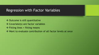
coef(lm1)[1] + coef(lm1)[2]*80
newdata <- data.frame(parent=80)
predict(lm1,newdata)](https://image.slidesharecdn.com/dataminingwithr-regression-131231060253-phpapp02/85/Data-mining-with-R-regression-models-16-320.jpg)
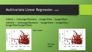
![Multivariate Linear Regression
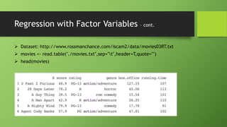
WHO childhood hunger data
Dataset:
http://apps.who.int/gho/athena/data/GHO/WHOSIS_000008.csv?pr
ofile=text&filter=COUNTRY:*
hunger <- read.csv("./hunger.csv")
hunger <- hunger[hunger$Sex!="Both sexes", ]](https://image.slidesharecdn.com/dataminingwithr-regression-131231060253-phpapp02/85/Data-mining-with-R-regression-models-17-320.jpg)
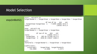


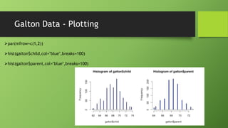
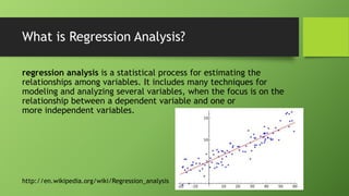
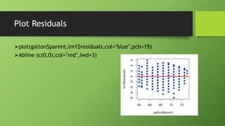
The document discusses data mining using R with a focus on regression models, demonstrating how to analyze and visualize relationships between variables using the Galton dataset. It explains the importance of model accuracy through measures such as p-values and confidence intervals, and introduces multivariate linear regression with examples. Additionally, it covers fitting models with factor variables and provides various data sources for practical applications.


