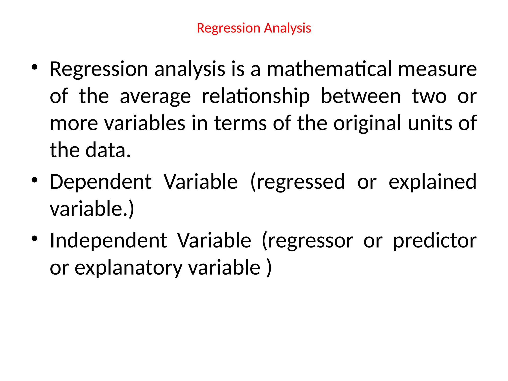
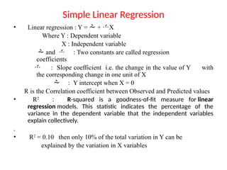
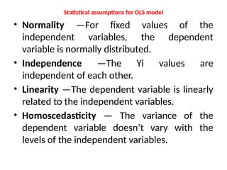
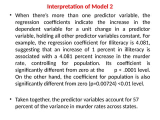
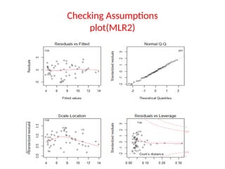
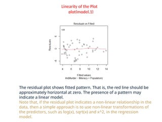
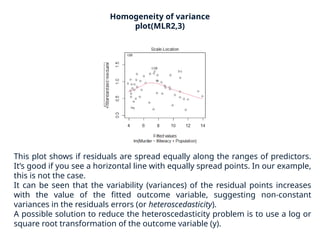
Regression Analysis
• Regression analysis is a mathematical measure
of the average relationship between two or
more variables in terms of the original units of
the data.
• Dependent Variable (regressed or explained
variable.)
• Independent Variable (regressor or predictor
or explanatory variable )
Simple Linear Regression
• Linear regression : Y =  + X
Where Y : Dependent variable
X : Independent variable
 and  : Two constants are called regression
coefficients
 : Slope coefficient i.e. the change in the value of Y with
the corresponding change in one unit of X
 : Y intercept when X = 0
R is the Correlation coefficient between Observed and Predicted values
• R2
: R-squared is a goodness-of-fit measure for linear
regression models. This statistic indicates the percentage of the
variance in the dependent variable that the independent variables
explain collectively.
.
• R2
= 0.10 then only 10% of the total variation in Y can be
explained by the variation in X variables
Statistical assumptions for OLS model
• Normality —For fixed values of the
independent variables, the dependent
variable is normally distributed.
• Independence —The Yi values are
independent of each other.
• Linearity —The dependent variable is linearly
related to the independent variables.
• Homoscedasticity — The variance of the
dependent variable doesn’t vary with the
levels of the independent variables.
• Click Regression icon
• Select Linear regression
• Bring dependent variable into dependent variable box and
bring independent scale variables into covariates box and
bring nominal independent variables into Factors box
• Under Model fit, select Fit measures and overall Model fit
• Click standardized estimates under model fit
• Under assumption option checks all assumptions
For Women Data
• From the output, you see that the prediction equation is
• Weight = −87.52 + 3.45 *Height, the regression coefficient (3.45) is
significantly different from zero(p < 0.001) and indicates that there’s an
expected increase of 3.45 pounds of weight for every 1 inch increase in
height.
• The multiple R-squared (0.991) indicates that the model accounts for 99.1
percent of the variance in weights. This fit is a good fit.
• The multiple R-squared is also the squared correlation between the actual
and predicted value.
• The residual standard error (1.53 lbs.) can be thought of as the average
error in predicting weight from height using this model.
• The F statistic tests whether the predictor variables taken together, predict
the response variable above chance levels.
• Because there’s only one predictor variable in simple regression, in this
example the F test is equivalent to the t-test for the regression coefficient
for height.
Multiple Linear Regression
• Ordinary Least Square regression fits models of
the form ; i=1,2,. . ., n
• Where n is the number of observations and k is
the number of predictor variables. In this equation
is the predicted value of the dependent variable
for observation i
• is the jth
predictor value for the ith
observation
• is the intercept and is the regression
coefficient for the jth predictor. Our aim is to
minimize the difference between observed value
and predicted value of the model.
In this model only variables Population and
Illiteracy are significant
Model2 contains only two significant
variables
Call:
lm(formula = Murder ~ Illiteracy + Population, data = state)
Residuals:
Min 1Q Median 3Q Max
-4.7652 -1.6561 -0.0898 1.4570 7.6758
Coefficients:
Estimate Std. Error t value Pr(>|t|)
(Intercept) 1.65154974 0.81011208 2.039 0.04713 *
Illiteracy 4.08073664 0.58481561 6.978 0.00000000883 ***
Population 0.00022419 0.00007984 2.808 0.00724 **
---
Signif. codes: 0 '***' 0.001 '**' 0.01 '*' 0.05 '.' 0.1 ' ' 1
Residual standard error: 2.481 on 47 degrees of freedom
Multiple R-squared: 0.5668, Adjusted R-squared: 0.5484
F-statistic: 30.75 on 2 and 47 DF, p-value: 0.000000002893
Interpretation of Model 2
• When there’s more than one predictor variable, the
regression coefficients indicate the increase in the
dependent variable for a unit change in a predictor
variable, holding all other predictor variables constant. For
example, the regression coefficient for Illiteracy is 4.081,
suggesting that an increase of 1 percent in illiteracy is
associated with a 4.081 percent increase in the murder
rate, controlling for population. Its coefficient is
significantly different from zero at the p < .0001 level.
On the other hand, the coefficient for population is also
significantly different from zero (p=0.00724) <0.01 level.
• Taken together, the predictor variables account for 57
percent of the variance in murder rates across states.
Checking Assumptions
plot(MLR2)
Linearity of the Plot
plot(model,1)
The residual plot shows fitted pattern. That is, the red line should be
approximately horizontal at zero. The presence of a pattern may
indicate a linear model.
Note that, if the residual plot indicates a non-linear relationship in the
data, then a simple approach is to use non-linear transformations of
the predictors, such as log(x), sqrt(x) and x^2, in the regression
model.
Homogeneity of variance
plot(MLR2,3)
This plot shows if residuals are spread equally along the ranges of predictors.
It’s good if you see a horizontal line with equally spread points. In our example,
this is not the case.
It can be seen that the variability (variances) of the residual points increases
with the value of the fitted outcome variable, suggesting non-constant
variances in the residuals errors (or heteroscedasticity).
A possible solution to reduce the heteroscedasticity problem is to use a log or
square root transformation of the outcome variable (y).
Normality of residuals
plot(MLR2,2)
The QQ plot of residuals can be used to visually check the normality
assumption. The normal probability plot of residuals should
approximately follow a straight line.
In our example, all the points fall approximately along this reference line
except point 28, so we can assume normality.
Outliers and high leverage points
Outliers:
An outlier is a point that has an extreme outcome variable value. The
presence of outliers may affect the interpretation of the model, because it
increases the RSE.
Outliers can be identified by examining the standardized
residual (or studentized residual), which is the residual divided by its
estimated standard error. Standardized residuals can be interpreted as the
number of standard errors away from the regression line.
Observations whose standardized residuals are greater than 3 in
absolute value are possible outliers (James et al. 2014).
High leverage points:
A data point has high leverage, if it has extreme predictor x values. This can
be detected by examining the leverage statistic or the hat-value. A value of
this statistic above 2(p + 1)/n indicates an observation with high leverage (P.
Bruce and Bruce 2017); where, p is the number of predictors and n is the
number of observations.
Outliers and high leverage points can be identified by inspecting
the Residuals vs Leverage plot:
Outliers and high leverage points
plot(MLR2,5)
The plot above highlights the only two most extreme points (#11,
#28), with a standardized residuals are nearly -1.5 and 3.0. However,
there is no outliers that exceed 3 standard deviations, what is good.
Additionally, there is 3 high leverage point in the data. That is, all
data points, have a leverage statistic below 2(p + 1)/n = 6/50 = 0.12.
Influential values
An influential value is a value, which inclusion or exclusion can
alter the results of the regression analysis. Such a value is
associated with a large residual.
Not all outliers (or extreme data points) are influential in linear
regression analysis.
Statisticians have developed a metric called Cook’s distance to
determine the influence of a value. This metric defines
influence as a combination of leverage and residual size.
A rule of thumb is that an observation has high influence if
Cook’s distance exceeds 4/(n - p - 1)(P. Bruce and Bruce 2017),
where n is the number of observations and p the number of
predictor variables.
The Residuals vs Leverage plot can help us to find influential
observations if any. On this plot, outlying values are generally
located at the upper right corner or at the lower right corner.
Those spots are the places where data points can be
par(mfrow=c(1,2))
plot(MLR2,4)
plot(MLR2,5)
By default, the top 3 most extreme values are labelled on the Cook’s
distance plot. If you want to label the top 5 extreme values, specify the
option id.n as follow:
plot(MLR2,id.n=5)
In our data only one observation value(28) Exceeds Cook’s Distance
4/(50-2-1)=0.08510638
• Keep this model as it

Regression_JAMOVI.pptx- Statistical data analysis

  • 1.
    Regression Analysis • Regressionanalysis is a mathematical measure of the average relationship between two or more variables in terms of the original units of the data. • Dependent Variable (regressed or explained variable.) • Independent Variable (regressor or predictor or explanatory variable )
  • 2.
    Simple Linear Regression •Linear regression : Y =  + X Where Y : Dependent variable X : Independent variable  and  : Two constants are called regression coefficients  : Slope coefficient i.e. the change in the value of Y with the corresponding change in one unit of X  : Y intercept when X = 0 R is the Correlation coefficient between Observed and Predicted values • R2 : R-squared is a goodness-of-fit measure for linear regression models. This statistic indicates the percentage of the variance in the dependent variable that the independent variables explain collectively. . • R2 = 0.10 then only 10% of the total variation in Y can be explained by the variation in X variables
  • 3.
    Statistical assumptions forOLS model • Normality —For fixed values of the independent variables, the dependent variable is normally distributed. • Independence —The Yi values are independent of each other. • Linearity —The dependent variable is linearly related to the independent variables. • Homoscedasticity — The variance of the dependent variable doesn’t vary with the levels of the independent variables.
  • 4.
    • Click Regressionicon • Select Linear regression • Bring dependent variable into dependent variable box and bring independent scale variables into covariates box and bring nominal independent variables into Factors box • Under Model fit, select Fit measures and overall Model fit • Click standardized estimates under model fit • Under assumption option checks all assumptions
  • 5.
  • 6.
    • From theoutput, you see that the prediction equation is • Weight = −87.52 + 3.45 *Height, the regression coefficient (3.45) is significantly different from zero(p < 0.001) and indicates that there’s an expected increase of 3.45 pounds of weight for every 1 inch increase in height. • The multiple R-squared (0.991) indicates that the model accounts for 99.1 percent of the variance in weights. This fit is a good fit. • The multiple R-squared is also the squared correlation between the actual and predicted value. • The residual standard error (1.53 lbs.) can be thought of as the average error in predicting weight from height using this model. • The F statistic tests whether the predictor variables taken together, predict the response variable above chance levels. • Because there’s only one predictor variable in simple regression, in this example the F test is equivalent to the t-test for the regression coefficient for height.
  • 8.
    Multiple Linear Regression •Ordinary Least Square regression fits models of the form ; i=1,2,. . ., n • Where n is the number of observations and k is the number of predictor variables. In this equation is the predicted value of the dependent variable for observation i • is the jth predictor value for the ith observation • is the intercept and is the regression coefficient for the jth predictor. Our aim is to minimize the difference between observed value and predicted value of the model.
  • 9.
    In this modelonly variables Population and Illiteracy are significant
  • 10.
    Model2 contains onlytwo significant variables
  • 11.
    Call: lm(formula = Murder~ Illiteracy + Population, data = state) Residuals: Min 1Q Median 3Q Max -4.7652 -1.6561 -0.0898 1.4570 7.6758 Coefficients: Estimate Std. Error t value Pr(>|t|) (Intercept) 1.65154974 0.81011208 2.039 0.04713 * Illiteracy 4.08073664 0.58481561 6.978 0.00000000883 *** Population 0.00022419 0.00007984 2.808 0.00724 ** --- Signif. codes: 0 '***' 0.001 '**' 0.01 '*' 0.05 '.' 0.1 ' ' 1 Residual standard error: 2.481 on 47 degrees of freedom Multiple R-squared: 0.5668, Adjusted R-squared: 0.5484 F-statistic: 30.75 on 2 and 47 DF, p-value: 0.000000002893
  • 12.
    Interpretation of Model2 • When there’s more than one predictor variable, the regression coefficients indicate the increase in the dependent variable for a unit change in a predictor variable, holding all other predictor variables constant. For example, the regression coefficient for Illiteracy is 4.081, suggesting that an increase of 1 percent in illiteracy is associated with a 4.081 percent increase in the murder rate, controlling for population. Its coefficient is significantly different from zero at the p < .0001 level. On the other hand, the coefficient for population is also significantly different from zero (p=0.00724) <0.01 level. • Taken together, the predictor variables account for 57 percent of the variance in murder rates across states.
  • 13.
  • 14.
    Linearity of thePlot plot(model,1) The residual plot shows fitted pattern. That is, the red line should be approximately horizontal at zero. The presence of a pattern may indicate a linear model. Note that, if the residual plot indicates a non-linear relationship in the data, then a simple approach is to use non-linear transformations of the predictors, such as log(x), sqrt(x) and x^2, in the regression model.
  • 15.
    Homogeneity of variance plot(MLR2,3) Thisplot shows if residuals are spread equally along the ranges of predictors. It’s good if you see a horizontal line with equally spread points. In our example, this is not the case. It can be seen that the variability (variances) of the residual points increases with the value of the fitted outcome variable, suggesting non-constant variances in the residuals errors (or heteroscedasticity). A possible solution to reduce the heteroscedasticity problem is to use a log or square root transformation of the outcome variable (y).
  • 16.
    Normality of residuals plot(MLR2,2) TheQQ plot of residuals can be used to visually check the normality assumption. The normal probability plot of residuals should approximately follow a straight line. In our example, all the points fall approximately along this reference line except point 28, so we can assume normality.
  • 17.
    Outliers and highleverage points Outliers: An outlier is a point that has an extreme outcome variable value. The presence of outliers may affect the interpretation of the model, because it increases the RSE. Outliers can be identified by examining the standardized residual (or studentized residual), which is the residual divided by its estimated standard error. Standardized residuals can be interpreted as the number of standard errors away from the regression line. Observations whose standardized residuals are greater than 3 in absolute value are possible outliers (James et al. 2014). High leverage points: A data point has high leverage, if it has extreme predictor x values. This can be detected by examining the leverage statistic or the hat-value. A value of this statistic above 2(p + 1)/n indicates an observation with high leverage (P. Bruce and Bruce 2017); where, p is the number of predictors and n is the number of observations. Outliers and high leverage points can be identified by inspecting the Residuals vs Leverage plot:
  • 18.
    Outliers and highleverage points plot(MLR2,5) The plot above highlights the only two most extreme points (#11, #28), with a standardized residuals are nearly -1.5 and 3.0. However, there is no outliers that exceed 3 standard deviations, what is good. Additionally, there is 3 high leverage point in the data. That is, all data points, have a leverage statistic below 2(p + 1)/n = 6/50 = 0.12.
  • 19.
    Influential values An influentialvalue is a value, which inclusion or exclusion can alter the results of the regression analysis. Such a value is associated with a large residual. Not all outliers (or extreme data points) are influential in linear regression analysis. Statisticians have developed a metric called Cook’s distance to determine the influence of a value. This metric defines influence as a combination of leverage and residual size. A rule of thumb is that an observation has high influence if Cook’s distance exceeds 4/(n - p - 1)(P. Bruce and Bruce 2017), where n is the number of observations and p the number of predictor variables. The Residuals vs Leverage plot can help us to find influential observations if any. On this plot, outlying values are generally located at the upper right corner or at the lower right corner. Those spots are the places where data points can be
  • 20.
    par(mfrow=c(1,2)) plot(MLR2,4) plot(MLR2,5) By default, thetop 3 most extreme values are labelled on the Cook’s distance plot. If you want to label the top 5 extreme values, specify the option id.n as follow: plot(MLR2,id.n=5) In our data only one observation value(28) Exceeds Cook’s Distance 4/(50-2-1)=0.08510638
  • 21.
    • Keep thismodel as it

Editor's Notes

  • #7 http://www.biostathandbook.com/linearregression.html