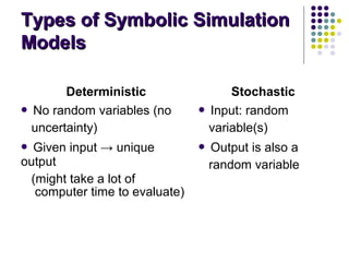
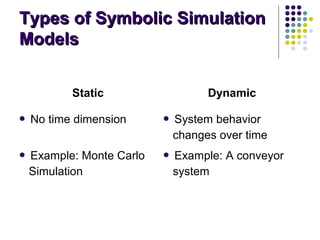
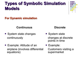
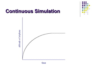
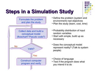
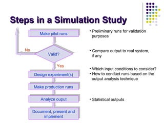
CS 8CS 85544
Computer SimulationComputer Simulation
Lecture Notes 01
Introduction to SimulationIntroduction to Simulation
 Simulation refers to a broad collection of methods
and applications to mimic the behavior of real
systems usually on a computer with appropriate
software.
 Simulation is the process of
 Formulating a model of the real system, and
 Conducting experiments with the model in order to
 understand (predict) the systems behavior, and
 evaluate various alternatives (design or
operational).
Introduction to SimulationIntroduction to Simulation
 System: Collection of elements working together
toward accomplishment of a specific objective.
 The facility or process of interest is usually called a
system.
 Ways to study a system include experimenting with
 the actual system, and
 a model of the system.
 Model: Simplified representation or abstraction of a
system.
Types of SimulationTypes of Simulation
 Iconic (physical) models
 Precise replica of an object (maybe in different
material or at smaller scale).
 Used primarily for training and research purposes.
 Examples:
Flight simulators (how to fly and handle emergency
situations)
Wind tunnels
Desktop manufacturing labs
 Symbolic models
 The real system is represented by mathematical equations
and logical relations.
 Basically computer simulation
Types of Symbolic SimulationTypes of Symbolic Simulation
ModelsModels
Deterministic Stochastic
 No random variables (no
uncertainty)
 Input: random
variable(s)
 Given input → unique
output
(might take a lot of
computer time to evaluate)
 Output is also a
random variable
Types of Symbolic SimulationTypes of Symbolic Simulation
ModelsModels
Static Dynamic
 No time dimension  System behavior
changes over time
 Example: Monte Carlo
Simulation
 Example: A conveyor
system
Types of Symbolic SimulationTypes of Symbolic Simulation
ModelsModels
Continuous Discrete
 System state changes
continuously
 System state
changes at discrete
points in time
 Example: Altitude of an
airplane (involves differential
equations)
 Example:
Customers visiting a
supermarket
For Dynamic simulationFor Dynamic simulation
Continuous SimulationContinuous Simulation
Discrete SimulationDiscrete Simulation
Monte Carlo (MC) SimulationMonte Carlo (MC) Simulation
 A random number (RN) is a random variable (RV) ~
Uniform (0,1)
 In Monte Carlo simulation, an iid sample of RNs is
obtained to solve a problem
Static, Stochastic MC SimulationStatic, Stochastic MC Simulation
Example: Estimation ofExample: Estimation of ππ
Area of the circle is π r2
= π
since r = 1
Area of shaded quarter-circle
= π/4
How can we use MC
simulation in estimating the
value of π ?
 Area of small square (in the main quadrant) = 1
 (Area of quarter-circle) / (Area of small square) = π/4
Algorithm:
 S1. Generate two RNs ~ uniform (0,1).
 S2. Using these as (x, y) coordinates of a point, find
the Euclidean distance, d, from the origin.
 S3. If d < 1 then the point is inside the quarter-circle,
otherwise it is outside the quarter-circle (but inside
the small square).
Static, Stochastic MC SimulationStatic, Stochastic MC Simulation
Example: Estimation ofExample: Estimation of ππ
Static, Stochastic MC SimulationStatic, Stochastic MC Simulation
Example: Estimation ofExample: Estimation of ππ
 Repeat (replicate) S1-S3 n times where n is a very
large number. (The points will be distributed
uniformly inside the small square.) Count the
number of times the generated point falls inside the
circle, nq. Then, is an estimate for π/4.
 95% confidence interval for π is :
nnp q /ˆ =
n
pp
p
)ˆ1(ˆ
)96.1(4ˆ4
−
±
Static, Stochastic MC SimulationStatic, Stochastic MC Simulation
Example: Estimation ofExample: Estimation of ππ
Empirical results (Seila et al., 2003, Applied Simulation Modeling)
Static, Stochastic MC SimulationStatic, Stochastic MC Simulation
Example: Estimation ofExample: Estimation of ππ
Plot showing convergence of estimates to π
1. Analytical Models: Represent the system by a set
of equations and logical relations. Some can be
solved analytically using algebra, calculus,
probability theory, e.g. LP models, queuing
models. Many real world problems are too
complex to be solved analytically.
2. Simulation: Often the only symbolic model
representing a complex system sufficiently. Yields
a different set of outputs (estimates) for each set of
inputs. No optimization in the strict sense.
Means of Analyzing a SystemMeans of Analyzing a System
Cone of AbstractionCone of Abstraction
Advantages andAdvantages and
Disadvantages of SimulationDisadvantages of Simulation
Advantages:
 Increased realism: Simulation is closer to reality
than analytical models. Fewer simplifying
assumptions are made. Hence, complex systems
can be modeled.
 Existing or non-existing systems can be studied.
New strategies for an existing system or a totally
new system can be studied without actually
investing in the physical system (great savings).
 Hazardous systems can be studied without risks.
Advantages andAdvantages and
Disadvantages of SimulationDisadvantages of Simulation
Advantages:
 Time compression or expansion is possible
 Bottleneck analysis can be performed
 “What if” questions can be answered
 Results are reproducible. No measurement errors
except round off.
Same random variates → same results.
Random variates: Realizations of an input random
variable generated during simulation.
Advantages andAdvantages and
Disadvantages of SimulationDisadvantages of Simulation
Advantages:
 Good control on experimental conditions
 to eliminate undesired sources of variability, and
 to try alternatives under identical conditions
 Ease of communication with the management,
especially with the help of animation.
Advantages andAdvantages and
Disadvantages of SimulationDisadvantages of Simulation
Disadvantages:
 Model building requires special training and data
collection
 Statistical analysis: Stochasticity requires more and
longer runs and special knowledge for analysis
 Expensive and time consuming to develop, code
and analyze
 No exact solutions are obtained. Results are only
estimates
Advantages andAdvantages and
Disadvantages of SimulationDisadvantages of Simulation
Disadvantages:
 Lack of generality: Results are valid only for a
particular configuration of a particular system (given
results for 3 servers, we cannot extrapolate for n
servers)
 Lack of optimization
Don’t Simulate When…Don’t Simulate When…
(Banks and Gibson, 1997, IIE Solutions)
 The problem can be solved using “common sense
analysis” (simple calculations), e.g. if customers
arrive at an average rate of 100/hr and they are
served at a mean rate of 12/hr, then we need
100/12 = 8.33 ~ 9 servers
 The problem can be solved analytically, e.g.
average waiting time of customers in system can be
found analytically for M/M/s queueing systems
 Direct experimentation in real system is easier, e.g.
direct observation in a drive-in fast food restaurant
Don’t Simulate When…Don’t Simulate When…
(Banks and Gibson, 1997, IIE Solutions)
 Cost of simulation exceeds possible savings
 Resources are not available
 The model cannot be verified or validated
 Project expectations cannot be met (do not
overpromise)
 The system behavior is too complex or cannot be
defined (ill-structured problem)
Don’t Simulate When…Don’t Simulate When…
Simulation projects cost money, but can produce a
significant return on investment when conducted
properly. If the project is successful then the money is
well spent, and this will promote the technology. If the
project is not successful, it hurts the reputation of
simulation and, by association, each of us.
Steps in a Simulation StudySteps in a Simulation Study
Collect data and build a
conceptual model
(flowchart? Pseudo code?)
Collect data and build a
conceptual model
(flowchart? Pseudo code?)
Formulate the problem
and plan the study
Formulate the problem
and plan the study
Yes
No
Valid?Valid?
Construct computer
program and verify
Construct computer
program and verify
• Define the problem (system and
environment) nad objectives
• Plan the study (team, cost, time)
• Probability distribution of input
random variables
• Start with simple, build up as
necessary
• Does the conceptual model
represent reality? (Talk to system
people)
• Choice of language
• Test if the program does what
you intend it to do
Steps in a Simulation StudySteps in a Simulation Study
• Preliminary runs for validation
purposes
• Which input conditions to consider?
• How to conduct runs based on the
output analysis technique
• Statistical outputs
• Compare output to real system,
if any
Document, present and
implement
Document, present and
implement
Make pilot runsMake pilot runs
Yes
No
Valid?Valid?
Design experiment(s)Design experiment(s)
Make production runsMake production runs
Analyze ouputAnalyze ouput
Elements in a SimulationElements in a Simulation
StudyStudy
 Entities: Objects of interest (customers, jobs, etc.)
that flow through the system.
An entity is characterized by its attributes and
usually interacts with resources.
 Events: An occurrence (arrival, service completion,
etc.) that changes the system state.
 Input parameters (constants or random variables):
 Uncontrollable, e.g. time between customer arrivals
 Controllable, e.g. number of parallel servers
Elements in a SimulationElements in a Simulation
StudyStudy
State variables: Variables that define system state
at any given time, e.g. number of customers in
system, number of busy servers.
Performance measures: Output statistics used to
evaluate objectives, e.g. average waiting time of
customers in system, percentage utilization of
servers.
Alternative strategies to be evaluated.
In developing our conceptual model, we must
identify/determine the above.
Examples of System andExamples of System and
ComponentsComponents
SystemSystem EntitiesEntities AttributesAttributes ActivitiesActivities EventsEvents State VariablesState Variables
Banking Customers
Checking
account
balance
Making
deposits
Arrival,
departure
Number of busy teller, number
of waiting customer
Rapid rail Riders
Origination,
destination
Traveling
Arrival at
station
Number of riders waiting at
each station, number of riders
in transit
Production Jobs
Arrival time,
process time(s)
Welding,
stamping
Completion
of welding,
breakdown
Status of machines (busy, idle
or down)
Communications Messages
Message
length,
destination
Transmitting
Arrival at
destination
Number of messages waiting to
be transmitted
Inventory Orders
Order quantity,
due date
Withdrawing
renewing
Demand
Levels of inventory, backlogged
demand

Cs854 lecturenotes01

  • 1.
    CS 8CS 85544 ComputerSimulationComputer Simulation Lecture Notes 01
  • 2.
    Introduction to SimulationIntroductionto Simulation  Simulation refers to a broad collection of methods and applications to mimic the behavior of real systems usually on a computer with appropriate software.  Simulation is the process of  Formulating a model of the real system, and  Conducting experiments with the model in order to  understand (predict) the systems behavior, and  evaluate various alternatives (design or operational).
  • 3.
    Introduction to SimulationIntroductionto Simulation  System: Collection of elements working together toward accomplishment of a specific objective.  The facility or process of interest is usually called a system.  Ways to study a system include experimenting with  the actual system, and  a model of the system.  Model: Simplified representation or abstraction of a system.
  • 4.
    Types of SimulationTypesof Simulation  Iconic (physical) models  Precise replica of an object (maybe in different material or at smaller scale).  Used primarily for training and research purposes.  Examples: Flight simulators (how to fly and handle emergency situations) Wind tunnels Desktop manufacturing labs  Symbolic models  The real system is represented by mathematical equations and logical relations.  Basically computer simulation
  • 5.
    Types of SymbolicSimulationTypes of Symbolic Simulation ModelsModels Deterministic Stochastic  No random variables (no uncertainty)  Input: random variable(s)  Given input → unique output (might take a lot of computer time to evaluate)  Output is also a random variable
  • 6.
    Types of SymbolicSimulationTypes of Symbolic Simulation ModelsModels Static Dynamic  No time dimension  System behavior changes over time  Example: Monte Carlo Simulation  Example: A conveyor system
  • 7.
    Types of SymbolicSimulationTypes of Symbolic Simulation ModelsModels Continuous Discrete  System state changes continuously  System state changes at discrete points in time  Example: Altitude of an airplane (involves differential equations)  Example: Customers visiting a supermarket For Dynamic simulationFor Dynamic simulation
  • 8.
  • 9.
  • 10.
    Monte Carlo (MC)SimulationMonte Carlo (MC) Simulation  A random number (RN) is a random variable (RV) ~ Uniform (0,1)  In Monte Carlo simulation, an iid sample of RNs is obtained to solve a problem
  • 11.
    Static, Stochastic MCSimulationStatic, Stochastic MC Simulation Example: Estimation ofExample: Estimation of ππ Area of the circle is π r2 = π since r = 1 Area of shaded quarter-circle = π/4 How can we use MC simulation in estimating the value of π ?
  • 12.
     Area ofsmall square (in the main quadrant) = 1  (Area of quarter-circle) / (Area of small square) = π/4 Algorithm:  S1. Generate two RNs ~ uniform (0,1).  S2. Using these as (x, y) coordinates of a point, find the Euclidean distance, d, from the origin.  S3. If d < 1 then the point is inside the quarter-circle, otherwise it is outside the quarter-circle (but inside the small square). Static, Stochastic MC SimulationStatic, Stochastic MC Simulation Example: Estimation ofExample: Estimation of ππ
  • 13.
    Static, Stochastic MCSimulationStatic, Stochastic MC Simulation Example: Estimation ofExample: Estimation of ππ  Repeat (replicate) S1-S3 n times where n is a very large number. (The points will be distributed uniformly inside the small square.) Count the number of times the generated point falls inside the circle, nq. Then, is an estimate for π/4.  95% confidence interval for π is : nnp q /ˆ = n pp p )ˆ1(ˆ )96.1(4ˆ4 − ±
  • 14.
    Static, Stochastic MCSimulationStatic, Stochastic MC Simulation Example: Estimation ofExample: Estimation of ππ Empirical results (Seila et al., 2003, Applied Simulation Modeling)
  • 15.
    Static, Stochastic MCSimulationStatic, Stochastic MC Simulation Example: Estimation ofExample: Estimation of ππ Plot showing convergence of estimates to π
  • 16.
    1. Analytical Models:Represent the system by a set of equations and logical relations. Some can be solved analytically using algebra, calculus, probability theory, e.g. LP models, queuing models. Many real world problems are too complex to be solved analytically. 2. Simulation: Often the only symbolic model representing a complex system sufficiently. Yields a different set of outputs (estimates) for each set of inputs. No optimization in the strict sense. Means of Analyzing a SystemMeans of Analyzing a System
  • 17.
  • 18.
    Advantages andAdvantages and Disadvantagesof SimulationDisadvantages of Simulation Advantages:  Increased realism: Simulation is closer to reality than analytical models. Fewer simplifying assumptions are made. Hence, complex systems can be modeled.  Existing or non-existing systems can be studied. New strategies for an existing system or a totally new system can be studied without actually investing in the physical system (great savings).  Hazardous systems can be studied without risks.
  • 19.
    Advantages andAdvantages and Disadvantagesof SimulationDisadvantages of Simulation Advantages:  Time compression or expansion is possible  Bottleneck analysis can be performed  “What if” questions can be answered  Results are reproducible. No measurement errors except round off. Same random variates → same results. Random variates: Realizations of an input random variable generated during simulation.
  • 20.
    Advantages andAdvantages and Disadvantagesof SimulationDisadvantages of Simulation Advantages:  Good control on experimental conditions  to eliminate undesired sources of variability, and  to try alternatives under identical conditions  Ease of communication with the management, especially with the help of animation.
  • 21.
    Advantages andAdvantages and Disadvantagesof SimulationDisadvantages of Simulation Disadvantages:  Model building requires special training and data collection  Statistical analysis: Stochasticity requires more and longer runs and special knowledge for analysis  Expensive and time consuming to develop, code and analyze  No exact solutions are obtained. Results are only estimates
  • 22.
    Advantages andAdvantages and Disadvantagesof SimulationDisadvantages of Simulation Disadvantages:  Lack of generality: Results are valid only for a particular configuration of a particular system (given results for 3 servers, we cannot extrapolate for n servers)  Lack of optimization
  • 23.
    Don’t Simulate When…Don’tSimulate When… (Banks and Gibson, 1997, IIE Solutions)  The problem can be solved using “common sense analysis” (simple calculations), e.g. if customers arrive at an average rate of 100/hr and they are served at a mean rate of 12/hr, then we need 100/12 = 8.33 ~ 9 servers  The problem can be solved analytically, e.g. average waiting time of customers in system can be found analytically for M/M/s queueing systems  Direct experimentation in real system is easier, e.g. direct observation in a drive-in fast food restaurant
  • 24.
    Don’t Simulate When…Don’tSimulate When… (Banks and Gibson, 1997, IIE Solutions)  Cost of simulation exceeds possible savings  Resources are not available  The model cannot be verified or validated  Project expectations cannot be met (do not overpromise)  The system behavior is too complex or cannot be defined (ill-structured problem)
  • 25.
    Don’t Simulate When…Don’tSimulate When… Simulation projects cost money, but can produce a significant return on investment when conducted properly. If the project is successful then the money is well spent, and this will promote the technology. If the project is not successful, it hurts the reputation of simulation and, by association, each of us.
  • 26.
    Steps in aSimulation StudySteps in a Simulation Study Collect data and build a conceptual model (flowchart? Pseudo code?) Collect data and build a conceptual model (flowchart? Pseudo code?) Formulate the problem and plan the study Formulate the problem and plan the study Yes No Valid?Valid? Construct computer program and verify Construct computer program and verify • Define the problem (system and environment) nad objectives • Plan the study (team, cost, time) • Probability distribution of input random variables • Start with simple, build up as necessary • Does the conceptual model represent reality? (Talk to system people) • Choice of language • Test if the program does what you intend it to do
  • 27.
    Steps in aSimulation StudySteps in a Simulation Study • Preliminary runs for validation purposes • Which input conditions to consider? • How to conduct runs based on the output analysis technique • Statistical outputs • Compare output to real system, if any Document, present and implement Document, present and implement Make pilot runsMake pilot runs Yes No Valid?Valid? Design experiment(s)Design experiment(s) Make production runsMake production runs Analyze ouputAnalyze ouput
  • 28.
    Elements in aSimulationElements in a Simulation StudyStudy  Entities: Objects of interest (customers, jobs, etc.) that flow through the system. An entity is characterized by its attributes and usually interacts with resources.  Events: An occurrence (arrival, service completion, etc.) that changes the system state.  Input parameters (constants or random variables):  Uncontrollable, e.g. time between customer arrivals  Controllable, e.g. number of parallel servers
  • 29.
    Elements in aSimulationElements in a Simulation StudyStudy State variables: Variables that define system state at any given time, e.g. number of customers in system, number of busy servers. Performance measures: Output statistics used to evaluate objectives, e.g. average waiting time of customers in system, percentage utilization of servers. Alternative strategies to be evaluated. In developing our conceptual model, we must identify/determine the above.
  • 30.
    Examples of SystemandExamples of System and ComponentsComponents SystemSystem EntitiesEntities AttributesAttributes ActivitiesActivities EventsEvents State VariablesState Variables Banking Customers Checking account balance Making deposits Arrival, departure Number of busy teller, number of waiting customer Rapid rail Riders Origination, destination Traveling Arrival at station Number of riders waiting at each station, number of riders in transit Production Jobs Arrival time, process time(s) Welding, stamping Completion of welding, breakdown Status of machines (busy, idle or down) Communications Messages Message length, destination Transmitting Arrival at destination Number of messages waiting to be transmitted Inventory Orders Order quantity, due date Withdrawing renewing Demand Levels of inventory, backlogged demand