Basics Of Modeling And Simulation, Simulation Software
1.
Course Notes for
CS1538
Introduction to Simulation
By
John C. Ramirez
Department of Computer Science
University of Pittsburgh
2.
2
• These notesare intended for use by students in CS1538 at the
University of Pittsburgh and no one else
• These notes are provided free of charge and may not be sold in any
shape or form
• These notes are NOT a substitute for material covered during course
lectures. If you miss a lecture, you should definitely obtain both
these notes and notes written by a student who attended the lecture.
• Material from these notes is obtained from various sources,
including, but not limited to, the following:
4 Discrete-Event System Simulation, Fifth Edition by Banks, Carson, Nelson
and Nicol (Prentice Hall)
• Also (same title and authors) Third and Fourth Editions
4 Object-Oriented Discrete-Event Simulation with Java by Garrido (Kluwer
Academic/Plenum Publishers)
4 Simulation Modeling and Analysis, Third Edition by Law and Kelton
(McGraw Hill)
4 A First Course in Monte Carlo by George S. Fishman (Thomson & Brooks/
Cole
3.
3
Goals of Course
•To understand the basics of computer
simulation, including:
4 Simulation concepts and terminology
4 When it is useful
4 Why it is useful
4 How to approach a simulation
4 How to develop / run a simulation
4 How to interpret / analyze the results
4.
4
Goals of Course
•To understand and utilize some of the
mathematics required in simulations
4 Statistical models and probability
distributions
• How various models are defined
• Which models are correct for which situations
4 Simple queuing theory
• Characteristics
• Performance measures
• Markovian models
5.
5
Goals of Course
4Random number theory
• Generating and testing pseudo-random numbers
• Generating pseudo-random values within various
distributions
4 Analysis / generation of input data
• How is input data generated?
• Is the data correct and appropriate for the
simulation?
4 Analysis / measurement of output data
• What does the output data mean and what can be
derived from it?
• How confident are we in our results?
6.
6
Goals of Course
•To implement some simulation tools and
some simulation projects
4 What enhancements do typical
programming languages need to facilitate
simulation?
4 Programming will be done in Java
• Review if you are rusty
• Find / keep a good Java reference
• There are special-purpose simulation languages,
but we will probably not be using them
7.
7
Introduction to Simulation
•What is simulation?
4 Banks, et al:
• "A simulation is the imitation of the operation of a
real-world process or system over time". It
"involves the generation of an artificial history of
a system, and the observation of that artificial
history to draw inferences … "
4 Law & Kelton:
• "In a simulation we use a computer to evaluate a
model (of a system) numerically, and data are
gathered in order to estimate the desired true
characteristics of the model"
8.
8
Introduction to Simulation
4More specifically (but still superficially)
• We develop a model of some real-world system
that (we hope) represents the essential
characteristics of that system
– Does not need to exactly represent the system –
just the relevant parts
• We use a program (usually) to test / analyze that
model
– Carefully choosing input and output
• We use the results of the program to make some
deductions about the real-world system
4 http://en.wikipedia.org/wiki/Computer_simulation
• Some interesting info here
9.
9
Introduction to Simulation
•Why (or when) do we use simulation?
• This is fairly intuitive
4 Consider arbitrary large system X
• Could be a computer system, a highway, a
factory, a space probe, etc.
4 We'd like to evaluate X under different
conditions
• Option 1: Build system X and generate the
conditions, then examine the results
– This is not always feasible for many reasons:
> X may be difficult to build
> X may be expensive to build
10.
10
Introduction to Simulation
>We may not want to build X unless it is "worthwhile"
> The conditions that we are testing may be difficult or
expensive to generate for the real system
• For example:
– A company needs to increase its production and
needs to decide whether it should build a new
plant or it should try to increase production in the
plants it already has
> Which option is more cost-effective for the
company?
– Clearly, building the new plant would be very
expensive and would not be desirable to do unless
it is the more cost-effective solution
– But how can we know this unless we have built the
new plant?
11.
11
Introduction to Simulation
•Another (ongoing) example:
– NASA wants to know if damage on the Space
Shuttle will threaten it upon re-entry
– If they wait until re-entry to make a judgment, it is
already too late
– In this case it is not feasible to do the real-world
test
12.
12
Introduction to Simulation
•Option 2: Model system X, simulate the conditions
and use the simulation results to decide
– Continuing with the same first example:
– Model both possibilities for increasing production
and simulate them both
> We then choose the solution that is most
economically feasible
– Continuing with the Space Shuttle example
– Model the damage and the stress that re-entry
imparts on the shuttle
> Determine via a simulation if the damage will
threaten the shuttle or not
> Note the importance of being correct here
13.
13
Introduction to Simulation
•Clearly, this is itself not a trivial task
– Simulations are often large, complex and difficult
to develop
– Just developing the correct system model can be a
daunting task
> There are many variables that must be taken into
account
– However, if a new plant costs hundreds of millions
or even billions of dollars, spending on the order of
thousands (or even hundreds of thousands) of
dollars on a simulation could be a bargain
– Note that with the Shuttle example, most of the
work for this must be done in advance
> Don't have time to design & implement this during
the duration of a flight
14.
14
Introduction to Simulation
4When is simulation NOT a good idea?
– See Section 1.2 of Banks text
– We will look at some of the guidelines now
• Don't use a simulation when the problem can be
solved in a "simpler" or more exact way
– Some things that we think may have to be
simulated can be solved analytically
– Ex: Given N rolls of a fair pair of dice, what are the
relative expected frequencies of each of the
possible values {2, 3, 4, … 12} ?
> We could certainly simulate this, "rolling" the dice N
times and counting
> However, based on the probability of each possible
result, we can derive a more exact answer analytically
15.
15
Introduction to Simulation
>How many ways do we have of obtaining each
outcome?
2:1, 3:2, 4:3, 5:4, 6:5, 7:6, 8:5, 9:4, 10:3, 11:2, 12:1
Total of 36 possible outcomes
For N "rolls", the expected frequency of value i is
N * (Pi) = N * (outcomes yielding i / total outcomes)
> For example, for 900 rolls, the expected number of 9s
generated would be 900 * (4 / 36) = 100
> Note that the expected value may not be a whole
number (nor should it necessarily be)
> Given 500 rolls, the expected number of 9s is
500 * (4 / 36) 55.55
– Note: You should be familiar with the general
approach above from CS 0441
> We will be looking at some more complex analytical
models later on
16.
16
Introduction to Simulation
•Don't use a simulation if it is easier or cheaper to
experiment directly on a real system
– Ex: A 24 hour supermarket manager wants to know
how to best handle the cash register during the
"midnight shift":
> Have one cashier at all times
> Have two cashiers at all times
> Have one cashier at all times, and a second cashier
available (but only working as cashier if the line gets
too long)
– Each of these can be done during operating hours
> An extra employee can be used to keep track of
queue data (and would not be too expensive)
> Differences are (likely) not that drastic so that
customers will be alienated
17.
17
Introduction to Simulation
•Don't use a simulation if the system is too
complex to model correctly / accurately
– This is often not obvious
– Can depend on cost and alternatives as well
> However, a bad model may not be helpful and could
actually be harmful
> Ex: With the Space Shuttle, lives were at risk – if the
model predicts incorrectly the results are
catastrophic
18.
18
Some Definitions
• System
4"A group of objects that are joined together
in some regular interaction or
interdependence toward the
accomplishment of some purpose" (Banks et
al)
• Note that this is a very general definition
• We will represent this system in our simulation
using variables (objects) and operations
4 The state of a system is the variables (and
their values) at one instance in time
19.
19
Some Definitions
• Discretevs. Continuous Systems
4 Discrete System
Discrete System
• State variables change at discrete points in time
– Ex: Number of students in CS 1538
> When a registration or add is completed, number of
students increases, and when a drop is completed,
number of students decreases
4 Continuous System
• State variables change continuously over time
– Ex: Volume of CO2 in the atmosphere
> CO2 is being generated via people (breathing),
industries and natural events and is being
consumed by plants
20.
20
Some Definitions
– Modelsof continuous systems typically use
differential equations to indicate rate of change of
state variables
– Note that if we make the time increment and the
unit of measurement small enough, we may be
able to convert a continuous system into a discrete
one
> However, this may not be feasible to do
> Why?
– Also note that systems are not necessarily
exclusively discrete or exclusively continuous
• We will be primarily concerned with Discrete
Systems in this course
21.
21
Some Definitions
• SystemComponents
4 Entities
• Objects of interest within a system
– Typically "active" in some way
– Ex: Customers, Employees, Devices, Machines, etc
• Contain attributes to store information about them
– Ex: For Customer: items purchased, total bill
• May perform activities while in the system
– Ex: For Customer: shopping, paying bill
– In many cases it is really just the period of time
required to perform the activity
• Note how nicely this meshes with object-oriented
programming
22.
22
Some Definitions
4 Events
•Instantaneous occurrences that may change the
state of a system
– Note that the event itself does not take any time
– Ex: A customer arrives at a store
– Note that they "may" change the state of the system
> Example of when they would not?
• Endogenous event
– Events occurring within the system
– Ex: Customer moves from shopping to the check-out
• Exogenous event
– Events relating / connecting the system to the outside
– Ex: Customer enters or leaves the store
23.
23
Some Definitions
• SystemModel
4 A representation of the system to be used /
studied in place of the actual system
• Allows us to study a system without actually building
it (which, as we discussed previously, could be very
expensive and time-consuming to do)
4 Physical Model
• A physical representation of the system (often scaled
down) that is actually constructed
– Tests are then run on the model and the results used
to make decisions about the system
– Ex: Development of the "bouncing bomb" in WWII
> http://www.sirbarneswallis.com/Bombs.htm
– Ex: Most things done on Mythbusters
24.
24
Some Definitions
4 MathematicalModel
Mathematical Model
• Representing the system using logical and
mathematical relationships
• Simple ex: d = vot + ½ at2
– This equation can be used to predict the distance
traveled by an object at time t
– However, will acceleration always be the same?
• Often this model is fairly complex and defined by
the entities and events
• This is the model we will be using
• However, in order to be useful, the model must be
evaluated in some way
– i.e. The behavior based on the model must be
determined
25.
25
Some Definitions
• Analyticalevaluation
– If the model is not too complex we can sometimes
solve it in a closed form using analytical methods
– One type of analytical evaluation is the Markov
process (or Markov chain)
– Nice simple example at:
http://en.wikipedia.org/wiki/Examples_of_Markov_chains
– We will see this more in Section 6.4
– Often problems that are too complex, even if they
can be modeled analytically, are too computation
intensive to be practical
• Simulation evaluation
– More often we need to simulate the behavior of
the model
26.
26
Some Definitions
4 DeterministicModel
• Inputs to the simulation are known values
– No random variables are used
– Ex: Customer arrivals to a store are monitored over a
period of days and the arrival times are used as input
to the simulation
4 Stochastic Model
Stochastic Model
• One or more random variables are used in the
simulation
– Results can only be interpreted as estimates (or
educated guesses) of the true behavior of the system
– Quality of the simulation depends heavily on the
correctness of the random data distribution
> Different situations may require different distributions
27.
27
Some Definitions
– Ex:Customers arrive at a store with exponentially
distributed interarrival times having a mean of 5
minutes
• In most cases we do not know all of the input data
in advance, and at least some random data is
required
– Thus, our simulations will typically use the
stochastic model
28.
28
Some Definitions
4 StaticModel
• Models a system at a single point in time, rather
than over a period of time
• Sometimes called Monte Carlo simulations
– We'll briefly discuss these later (they are interesting
and very useful)
4 Dynamic Model
Dynamic Model
• Models a system over time
• Our simulations will typically use this model
• In summary our models will typically be:
discrete, mathematical, stochastic and
dynamic
29.
29
The Clock
• Sincewe are using the dynamic model, we
need to represent the passage of time
4 We need to use a clock
4 Three fundamental approaches to time
progression
• Next-event time advance
– Clock initialized to zero
– As the times of future events are determined, they
are put into the future event list (FEL)
– Clock is advanced to the time of the next most
imminent event, the event is executed and removed
from the list
– See example in Section 3.1.1
30.
30
The Clock
4 Ex:People (P) using a MAC machine
• Event A == arrival of a customer at MAC machine
• Event C == completion of a transaction by a customer
Clock FEL Event Action
0 (A2,t1), (C1,t2) A1
P1 arrives, is served; Events A2 and
C1 generated, placed in FEL
t1 (C1,t2), (A3,t3) A2
P2 arrives, waits; Event A3
generated, placed in FEL
t2 (A3,t3), (C2,t4) C1
P1 completes; P2 is served; Event C2
generated, placed in FEL
t3 (A4,t5), (C2,t4) A3
P3 arrives, waits; Event A4
generated, placed in FEL (note:
t5<t4)
t5 (C2,t4), (A5,t6) A4
P4 arrives, waits; Event A5
generated, placed in FEL
t4 (A5,t6), (C3,t7) C2
P2 completes; P3 is served; Event C3
generated, place in FEL
31.
31
The Clock
• Fixed-incrementtime advance (activity scanning)
– Clock initialized to zero
– Clock is incremented by a fixed amount (ex. 1)
– With each increment, list of events is checked to
see which should occur (could be none)
– Clock is typically easier to implement in this way
– However, execution is less efficient, esp. if time
between events is large
> Potentially many scans for each event
32.
32
The Clock
• Process-interactionapproach
– Entities are associated with processes
– Processes interact as entities progress through
system
– Could delay while waiting for a resource, or during
an interaction with another process
> Can be implemented with multithreading or
multiprocessing
33.
33
Simple Example
• Let'sconsider a very simple example:
4 Single-Channel Queue (Example 2.5 in text)
• Small grocery store with a single checkout counter
• Customers arrive at the checkout at random
between 1 and 8 minutes apart (uniform)
• Service times at the counter vary from 1 to 6 minutes
– P(1) = 0.1, P(2) = 0.2, P(3) = 0.3, P(4) = 0.25
P(5) = 0.1, P(6) = 0.05
• Start with first customer arriving at time 0
• Run for a given number of customers (text uses 100)
• Calculate some results that may be useful
34.
34
Simple Example
4 Theentities are the customers
4 The system is discrete since states are
changed at specific points in time
• ex: a customer arrives or leaves
4 The model is mathematical (since we don't
have real customers)
4 The model is stochastic since we are
generating random arrivals and random
service times
4 The model is dynamic since we are
progressing in time
35.
35
Simple Example
4 Whatresults are we interested in?
• In this simple case we may want to know
– What fraction of customers have to wait in line
– What is the average amount of time that they wait
– What is the fraction of time the cashier is idle (or
busy)
• We probably want to do several runs and get
cumulative results over the runs (ex: averages)
• There are more complex statistics that may be
relevant
– We will discuss some of these later
36.
36
Simple Example
4 Wecan program this example, but in this
simple case we could also use a table or
spreadsheet to obtain our results
• Let's first look at an "Excel novice" approach to this
– See sim1.xls
• Although some of the spreadsheet formulas require
some thought, this is fairly simple to do
• Note that each row in the spreadsheet depends only
on some local data (generated in that row) and the
data in the previous row
– We do not need a "memory" of all rows
• Authors have a much nicer spreadsheet with macros
– See http://www.bcnn.net
37.
37
Programming a SimpleExample
• If we do program it, how would we do it?
4 Using Java, it is logical to do it in an object-
oriented way
4 Let's think about what is involved
• We need to represent our entities
– As text indicates, for this simple example we do not
have to explicitly represent them
– However, we can do it if we want to – and have our
Customers and CheckOut as simple Java objects
• We need to represent our events
– We need to store events in our Future Event List
(FEL) and we have two different kinds of events
(arrival of a customer, finish of a checkout)
38.
38
Programming a SimpleExample
> We need to distinguish between the different event
types (since different actions are taken for different
events)
> We need to order our events based on the
simulation clock time that they will occur
– Thus we probably need to explicitly represent the
events in some way
> Use classes and inheritance to represent the
different events
> This enables events to share characteristics but also
to be distinguished from each other
> So we need a event time instance variable and a
method to compare event times
> Look at SimEvent.java, ArrivalEvent.java,
CompletionEvent.java
39.
39
Priority Queue toRepresent the FEL
• We need to represent the FEL itself
– Since we are inserting items and then removing
them based on priority (earliest next time of an
event is removed first), we should use a priority
queue (PQ) with the following operations:
> add (Object e) – add a new Object to the PQ
> remove() – remove and return the Object with the
min (best) priority value
> peek() – return the Object with the min (best) priority
value without removing it
– It's also a good idea to have some helper methods
> size() – how many items are in the PQ
> isEmpty() – is the PQ empty
– There are variations of these ops depending on the
implementation, but the idea is the same
40.
40
Priority Queue toRepresent the FEL
– How to efficiently implement a Priority Queue?
> How about an unsorted array or linked list?
> add is easy but remove is hard – why? – discuss
> How about a sorted array or linked list?
> removeMin is easy but add is hard – why? – discuss
– Neither implementation is adequate in terms of
efficiency
> Note that the premise of a PQ is that everything that
is inserted is eventually removed
> Thus, with N adds you have N removes
> Discuss / show on board overall time required for
both implementations
> You may have seen this already in CS 1501
– Thus we need a better approach
> Implementation of choice is the Heap
41.
41
Heap Implementation ofa Priority Queue
– Idea of a Heap:
> Store data in a partially ordered complete binary
tree such that the following rule holds for EACH
node, V:
Priority(V) betterthan
Priority(LChild(V))
Priority(V) betterthan
Priority(RChild(V))
> This is called the HEAP PROPERTY
> Note that betterthan here often means smaller
> Note also that there is no ordering of siblings – this
is why the overall ordering is only a partial ordering
– ex:
10
30
40 70
90 45
20
80
35
85
42.
42
Heap Implementation ofa Priority Queue
– How to do our operations?
> peek() is easy – return the root
> add() and remove() are not so obvious
> Let's look at them separately
– add(Object e)
> We want to maintain the heap property
> However, we don't know where in advance the new
object will end up
> We also don't want a lot of rearranging or searching
if we can avoid it – remember time is key
> Solution: Add new object at the next open leaf in the
last level of the tree, then push the node UP the tree
until it is in the proper location
> This operation is called upHeap
> See example on board
43.
43
Heap Implementation ofa Priority Queue
– remove()
> Clearly, the min node is the root
> However, removing it will disrupt the tree greatly
> How can we solve this problem?
• Remember BST delete?
– Did not actually delete the root, but
rather the _______________ (fill in blank)
• We will do a similar thing with our Heap
– Copy the last leaf to the root and delete
(easily) the leaf node
– Then re-establish the heap property by a
downHeap
– See example on board
44.
44
Heap Implementation ofa Priority Queue
– Run-Time?
> Since our tree is complete, it is balanced and thus
for N nodes has a height of ~ lgN
> Thus upHeapand downHeap require no more than
~lgN time to complete
> Thus, if we have N adds and N removeMins, our total
run-time will be NlgN
> This is a SIGNIFICANT improvement of the simpler
implementations, especially for a long simulation
> Ex: Compare N2
with NlgN for N = 1M (= 220
)
– Note:
> For our simple example, a heap is probably not
necessary, since we have few items in our FEL at any
given time
> However, for more complex simulations, with many
different event types, a heap is definitely preferable
45.
45
Implementing a Heap
–How to Implement a Heap?
> We could use a linked binary tree, similar to that used
for BST
Will work, but we have overhead associated with
dynamic memory allocation and access
> But note that we are maintaining a complete binary
tree for our heap
> It turns out that we can easily represent a complete
binary tree using an array
We simply must map the tree locations onto the
array indexes in a reasonable / consistent way
– Idea:
> Number nodes row-wise starting at 0 (some
implementations start at 1)
> Use these numbers as index values in the array
46.
46
Implementing a Heap
>Now, for node at index i
> See example on board
– Now we have the benefit of a tree structure with the
speed of an array implementation
• So now should we write the code?
– No! Luckily, in JDK 1.5 a heap-based PriorityQueue
class has been provided!
– It's still a good idea to understand the
implementation, however
– Look at API
Parent(i) = floor((i-1)/2)
LChild(i) = 2i+1
RChild(i) = 2i+2
47.
47
Queue for WaitingCustomers
• We need to represent the queue (or line) of
customers waiting at the checkout
– This is a FIFO queue and can simply be
implemented in various ways
> We can use a circular array
> We can use a linked-list
– You should be already familiar with queue
implementations from CS 0445
– In JDK 1.5 Queue is an interface which is
implemented by the LinkedList class
> See API
> Q: Would a similar approach using an ArrayList also
be good?
48.
48
Programming a SimpleExample
• We need to represent the clock
– This is fairly easy – we can do it with an integer
> In some cases it might be better to use a double
• We need to implement some activities
– These are actually better defined as the time
required for activities to execute
– Typically interarrival times or service times, either
specified exactly (with deterministic model) or by
probability distributions (with stochastic model)
> In our case, we have the interarrival times of
customers and the time required for checkout,
specified by the distributions shown on pp. 45-46 of
the text
> We will discuss various distributions in more detail
later
49.
49
Programming a SimpleExample
4 Let's put this all together: GrocerySim.java
• This is a fairly object-oriented implementation,
using newer JDK 1.5 features
4 Note that there is also a Java version from
authors in Chapter 4
• Look over this one as well
• Does not utilize JDK 1.5 and not quite as object-
oriented
• The author also switches distributions in this
implementation
– Uses an exponential distribution for arrivals
– Uses a normal distribution for service times
> We will look at these later
50.
50
One More Example
•News Dealer's Problem
4 Example 2.7 in text
4 Simple inventory problem
• Each day new inventory is produced and used, but is
not carried over to successive days
• Thus, time is more or less removed from this
problem
4 Used where goods are only useful for a short
time
• Ex: newspaper, fresh food
4 In this case, our goal is to try to optimize our
profit
51.
51
News Dealer's Problem
4Specifics of the News Dealer's Problem
• Seller buys N newspapers per day for 0.33 each
• Seller sells newspapers for 0.50 each
• Unused papers are "scrapped' for 0.05 each
• If seller runs out, lost revenue is 0.17 for each not
sold paper
– Text says this is controversial, which is true
– How to predict how many would have been sold?
> Perhaps seller goes home when he/she runs out
> May be a goal to run out every day – easier than
returning the papers for scrap
• See sim2.xls
52.
52
News Dealer's Problem
4In fact we do we really need to simulate this
problem at all?
• The data is simple and highly mathematical
• Time is not involved
4 Let's try to come up with an analytical solution
to this problem
• We have two distributions, the second of which utilizes
the result of the first
• Let's calculate the expected values for random
variables using these distributions
– For a given discrete random variable X, the expected
value,
E(X) = Sum [xi p(xi)] (more soon in Chapter 5)
all i
53.
53
News Dealer's Problem
•Let our random variable, X, be the number of
newspapers sold
– Let's first consider the expected value for each of
the demands of good, fair and poor
Demand Probability Distribution
Demand Good Fair Poor
40 0.03 0.10 0.44
50 0.05 0.18 0.22
60 0.15 0.40 0.16
70 0.20 0.20 0.12
80 0.35 0.08 0.06
90 0.15 0.04 0.00
100 0.07 0.00 0.00
54.
54
News Dealer's Problem
•Egood(X) = (40)(0.03) + (50)(0.05) + (60)(0.15) +
(70)(0.20) + (80)(0.35) + (90)(0.15) +
(100)(0.07) = 75.2
• Efair(X) = (40)(0.10) + (50)(0.18) + (60)(0.40) +
(70)(0.20) + (80)(0.08) + (90)(0.04) +
(100)(0.00) = 61
• Epoor(X) = (40)(0.44) + (50)(0.22) + (60)(0.16) +
(70)(0.12) + (80)(0.06) + (90)(0.00) +
(100)(0.00) = 51.4
4 Now we need to use the second distribution
(of good, fair and poor days) to determine the
overall expected value
55.
55
News Dealer's Problem
•E(X) = (Egood(X))(0.35) + (Efair(X))(0.45) +
(Epoor(X))(0.20) = 64.05
4 Now we utilize the expected number of
newspapers sold to find results for each of
the potential number that we stock
• Let sales = expected value calculated above
• Let stock = number vendor purchases
• Let left = stock – sales (only if stock > sales, else 0)
• Let lost = sales – stock (only if sales > stock, else 0)
• Profit = (Min(sales,stock))(0.5) – (stock)(0.33) +
(left)(0.05) – (lost)(0.17)
56.
56
News Dealer's Problem
StockProfit
40 2.71
50 6.11
60 9.51
70 9.2
80 6.4
90 3.6
100 0.82
Expected profit
values for given
stock amounts
Note that this table
shows that 60 is
the best choice
(more or less
agreeing with the
simulation results)
57.
57
News Dealer's Problem
4Is this analytical solution correct?
• Not entirely
• We are using an expected value to derive another
expected value – oversimplifying the actual analysis
• The variance from the expected value will cause our
actual results to differ
• Note that the simulation results are almost identical
to the analytical for small and large inventories
• In the middle there is more variation and this is
where using the expected value is inadequate
• However, as a basis for choosing the best number
of papers to stock, it still works
58.
58
Other Simulation Examples
4There are other examples in Chapters 2 and
3
• Read over them carefully
• We may look at some of these types of
simulations later on in the term
59.
59
Simulation Software
• Simulationscan be written in any good
programming language
• However, many things that need to be
done in simulations can be built into
languages to make them easier
4 Random values from various probability
distributions
4 Tools for modeling
4 Tools for generating and analyzing output
4 Graphical tools for displaying results
60.
60
Simulation Software
4 Lookat the various described languages
4 Our simple queueing example (Example 2.5)
is shown using many of the languages
• Even if you don't completely understand all of the
code, look it over to note some differences
4 We may look at one of these packages later
in the term if we have time
61.
61
Probability and Statisticsin Simulation
• Why do we need probability and
statistics in simulation?
4 Needed to validate the simulation model
4 Needed to determine / choose the input
probability distributions
• Needed to generate random samples / values
from these distributions
4 Needed to analyze the output data / results
4 Needed to design correct / efficient
simulation experiments
62.
62
Experiments and SampleSpace
• Experiment
4 A process which could result in several
different outcomes
• Sample Space
4 The set of possible outcomes of a given
experiment
• Example:
4 Experiment: Rolling a single die
4 Sample Space: {1, 2, 3, 4, 5, 6}
• Another example?
63.
63
Random Variables
• RandomVariable
4 A function that assigns a real number to
each point in a sample space
4 Example 5.2:
• Let X be the value that results when a single die is
rolled
• Possible values of X are 1, 2, 3, 4, 5, 6
• Discrete Random Variable
4 A random variable for which the number of
possible values is finite or countably infinite
• Example 5.2 above is discrete – 6 possible values
64.
64
Random Variables andProbability Distribution
• Countably infinite means the values can be
mapped to the set of integers
– Ex: Flip a coin an arbitrary number of times. Let X
be the number of times the coin comes up heads
• Probability Distribution
4 For each possible value, xi, for discrete
random variable X, there is a probability of
occurrence, P(X = xi) = p(xi)
4 p(xi) is the probability mass function (pmf)
of X, and obeys the following rules:
– p(xi) >= 0 for all i
– = 1
i
all
i
x
p )
(
65.
65
Random Variables andProbability Distribution
4 The set of pairs (xi, p(xi)) is the probability
distribution of X
4 Examples:
• For Example 5.2 (assuming a fair die):
– Probability Distribution:
> {(1, 1/6), (2, 1/6), (3, 1/6), (4, 1/6), (5, 1/6), (6, 1/6)}
• From Example 2.5 for Service Times
– Probability Distribution:
> {(1, 0.1), (2, 0.2), (3, 0.3), (4, 0.25), (5, 0.1), (6, 0.05)}
• From Example 2.7 for Type of Newsday
– Probability Distribution:
> {(0, 0.35), (1, 0.45), (2, 0.20)}
> Note in this case we are assigning the values 0, 1, 2 to the
outcomes somewhat arbitrarily
66.
66
Cumulative Distribution
• CumulativeDistribution Function
4 The pmf gives probabilities for individual
values xi of random variable X
4 The cumulative distribution function (cdf),
F(x), gives the probability that the value of
random variable X is <= x, or
F(x) = P(X <= x)
4 For a discrete random variable, this can be
calculated simply by addition:
F(x) =
x
x
i
i
x
p )
(
67.
67
Cumulative Distribution
4 Propertiesof cdf, F:
1) F is non-decreasing
2)
3)
and
P(a < X b) = F(b) – F(a) for all a < b
4 Ex: Probability that a roll of two dice will
result in a value > 7?
• Discuss
4 Ex: Probability that 10 flips of a fair coin will
yield between 6 and 8 (inclusive) heads?
• Discuss
0
)
(
lim
x
F
x
1
)
(
lim
x
F
x
68.
68
Expected Value
• ExpectedValue (for discrete random variables)
4 Also called the mean
4 Ex: Expected value for roll of 2 fair dice?
E(X) = (2)(1/36) + (3)(2/36) + (4)(3/36) + (5)(4/36) + (6)
(5/36) + (7)(6/36) + (8)(5/36) + (9)(4/36) + (10)(3/36) +
(11)(2/36) + (12)(1/36)
= 7
• Note that in this case the expected value is an actual
value, but not necessarily
i
all
i
i x
p
x
X
E )
(
)
(
69.
69
Expected Value andVariance
4 If each value has the same "probability", we
often add the values together and divide by
the number of values to get the mean
(average)
• Ex: Average score on an exam
• Variance
4 We won't prove the identity, but it is useful
]
])
[
[(
)
( 2
X
E
X
E
X
V
)
10
.
5
(
2
2
)]
(
[
)
( Equation
X
E
X
E
70.
70
Expected Value andVariance
• In the original definition, we need to subtract the
mean from each of the X values before squaring
– So we need each X value to calculate the mean
AND AFTER the mean has been calculated
> Must look at them twice
• In the right side of the equation (Equation 5.10 in
the text), we need to calculate the mean of X and
the mean of the squares of X
– We can do this as we process the individual X
values and need to look at them only one time
• Ex: What is the variance of the following group of
exam scores: { 75, 90, 40, 95, 80 }
– Since each value occurs once, we can consider this
to have a uniform distribution
71.
71
Expected Value andVariance
• V(X) using original definition:
E(X) = (75+90+40+95+80)/5 = 76
V(X) = E[(X – E[X])2
] = [(75-76)2
+ (90-76)2
+ (40-76)2
+ (95-76)2
+ (80-76)2
]/5
= (1 + 196 + 1296 + 361 + 16)/5 =
374
• V(X) using Equation 5.10
E(X) = (75+90+40+95+80)/5 = 76
E(X2
) = (5625+8100+1600+9025+6400)/5 = 6150
V(X) = 6150 – (76)2
= 374
– Note that in this case we can add each number to
one sum and its square to another, so we can
calculate our overall answer with one a single
"look" at each number
72.
72
Discrete Distributions
• DiscreteDistributions of interest:
4 Bernoulli Trials and the Bernoulli Distribution
• Consider an experiment with the following properties
– n independent trials are performed
– each trial has two possible results – success or failure
– the probability of success, p and failure, q (= 1 – p) is
constant from trial to trial
– for random variable X, X = 1 for a success and X = 0 for
a failure
• Probability Distribution:
P(X = 1) = p
P(X = 0) = 1 – p = q
or 0 for all other values of X
73.
73
Bernoulli Distribution
• ExpectedValue
– E(X) = (0)(q) + (1)(p) = p
• Variance
– V(X) = [02
q + 12
p] – p2
= p(1 – p)
4 A single Bernoulli trial is not that interesting
• Typically, multiple trials are performed, from
which we can derive other distributions:
– Binomial Distribution
– Geometric Distribution
74.
74
Binomial Distribution
4 BinomialDistribution
• Given n Bernoulli trials, let random variable X denote
the number of successes in those trials
• Note that the order of the successes is not important,
just the number of successes
– Thus, we can achieve the same number of successes in
various different ways
– Since the trials are independent, we can multiply the
probabilities for each trial to get the overall probability
for the sequence
otherwise
n
x
q
p
x
n
x
p
x
n
x
,
0
,
,
1
,
0
,
)
(
75.
75
Binomial Distribution
• Recallthat the number of combinations of n items
taken x at a time is
• E(X) = np
– Discuss
• V(X) = npq
• Consider an example:
– Exercise 5.1
– Read
– Do solution on board
)!
(
!
!
x
n
x
n
x
n
76.
76
Binomial Distribution
• Consideragain coin-flip ex. on slide 67
• Generally speaking binomial distributions can be
used to determine the probability of a given
number of defective items in a batch, or the
probability of a given number of people having a
certain characteristic
– Ex: The trait of having a klinkled flooje occurs on
average in 10% of Kreptoplomians (krep-tō-plō'-
mē-əns). Given a group of 20 Kreptoplomians,
what is the probability that 3 of them have klinkled
floojes?
P(3) = (20 C 3)(0.1)3
(0.9)17
= (1140)(0.001)(0.1668)
= 0.1902
> Note that if we wanted "at least 3" the answer would
be different – how to calculate?
77.
77
Geometric Distribution
4 GeometricDistribution
• Given a sequence of Bernoulli trials, let X represent
the number of trials required until the first success
– i.e. we have x – 1 failures, followed by a success
– Note that the maximum probability for this is at X =
1, regardless of p and q
• E(X) = 1/p
• V(X) = q/p2
– We will omit the proofs of the above, since they are
fairly complex (involving series solutions)
otherwise
x
p
q
x
p
x
,
0
,
2
,
1
,
)
(
1
78.
78
Geometric Distribution
• Ex:What is the probability that the first
Kreptoplomian found to have a klinkled flooje will
be the 5th
Kreptoplomian overall?
(0.9)4
(0.1) = 0.0656
• Ex: The probability that a certain computer will fail
during any 1-hour period is 0.001
– What is the probability that the computer will
survive at least 3 hours?
> Here p = 0.001 and q = (1 – p) = 0.999
– Using a geometric distribution, we want to solve
P(X >= 4) = 1 – P(1) – P(2) – P(3)
= 1 – (0.001) – (0.999)(0.001)
– (0.999)2
(0.001)
= 0.997
79.
79
Geometric Distribution
• TheGeometric Distribution is memoryless
– Consider the following two scenarios where p =
probability that a component will fail in the next
hour. Assume the current hour is hour 0.
1) What is the probability that the component will fail by
the end of hour 3?
2) What is the probability that the component will fail by
the end of hour 6, given that it has not failed by the end
of hour 3 ?
> For 1) the solution is P(1) + P(2) + P(3)
> For 2), since the component did NOT fail by the end of
hour 3, and since the probability is for the next hour
(whatever that hour may be), the solution is the same
– We can prove this property with fairly simple algebra
> First we need one additional definition
80.
80
Geometric Distribution
• Theconditional probability of an event, A, given
that another event, B, has occurred is defined to
be:
• Applying this to the geometric distribution we get
– Clearly, if X > s+t, then X > s (since t cannot be
negative), so we get
)
(
)
(
)
|
(
B
P
B
A
P
B
A
P
)
(
])
[
]
([
)
|
(
s
X
P
s
X
t
s
X
P
s
X
t
s
X
P
)
(
)
(
)
|
(
s
X
P
t
s
X
P
s
X
t
s
X
P
81.
81
Geometric Distribution
– Considerthat P(X > s) =
– We can use similar logic to determine that
P(X > s + t) = qs+t
– Now our conditional probability becomes
– and thus we have shown that the geometric distribution is
memoryless
> We will see shortly that the exponential distribution is also
memoryless
1
1
1
1
1
1
)
1
(
s
j
j
j
s
j
j
s
j
j
q
q
q
q
p
q
s
s
s
s
s
s
s
q
q
q
q
q
q
q
3
2
2
1
1
)
(
)
|
( t
X
P
q
q
q
s
X
t
s
X
P t
s
t
s
82.
82
Poisson Distribution
4 PoissonDistribution
• Often used to model arrival processes with constant
arrival rates
• Gives (probability of) the number of events that
occur in a given period
• Formula looks quite complicated (and NOT discrete),
but it is discrete and using it is not that difficult
• Where is the mean arrival rate. Note that must
be positive
• E(X) = V(X) =
otherwise
x
x
e
x
p
x
,
0
,
1
,
0
,
!
)
(
83.
83
Poisson Distribution
• Note:The Poisson Distribution is actually the
convergence of the Binomial Distribution as the
number of trials, n, approaches infinity
– If we think of n as the number of subintervals of a
given unit of time
– As n , the subintervals get smaller and smaller
– We will skip the detailed math here
– One nice feature of this is that we can use a Poisson
Distribution to approximate a Binomial Distribution
when n is large
x
i
i
i
e
x
F
0 !
)
(
84.
84
Poisson Distribution
• Example
–Number of people logging onto a computer per
minute is Poisson Distributed with mean 0.7
– What is the probability that 5 or more people will
log onto the computer in the next 10 minutes?
– Solution?
>Must first convert the mean to the 10 minute period –
if mean is 0.7 in 1 minute, it will be (0.7)(10) = 7 in a ten
minute period
>Now we can plug in the formula
>P(X >= 5) = 1 – P(0) – P(1) – P(2) – P(3) – P(4)
= 1 – F(4) (where F is the
cdf)
= 1 – 0.173 (from Table A.4
in the text)
= 0.827
85.
85
Continuous Random Variables
•Continuous Random Variable
4 Random variable X is continuous if its sample
space is a range or collection of ranges of real
values
4 More formally, there exists non-negative function
f(x), called the probability density function, such
that for any set of real numbers, S
a) f(x) >= 0 for all x in the range space
b) – the total area under f(x) is 1
c) f(x) = 0 for all x not in the range space
– Note that f(x) does NOT give the probability that X = x
– Unlike the pmf for discrete random variables
space
range
dx
x
f 1
)
(
86.
86
Continuous Random Variables
•The probability that X lies in a given interval [a,b] is
– We see this visually as the "area under the curve"
– Note that for continuous random variables,
P(X = x) = 0 for any x (see from
formula above)
– Rather we always look at the probability of x within a
given range (although the range could be very small)
• The cumulative density function (cdf), F(x) is simply the
integral from - to x or
– This gives us the probability up to x
b
a
dx
x
f
b
X
a
P )
(
)
(
x
dt
t
f
x
F )
(
)
(
87.
87
Continuous Random Variables
•Ex: Consider the uniform distribution on the range
[a,b] (see text p. 189)
– Look at plots on board for example range [0,1]
> What about F(x) when x < a or x > b?
4 Expected Value for a continuous random variable
– Compare to the discrete expected value
otherwise
b
x
a
if
a
b
x
f
0
1
)
(
x
a
x
a
b
x
a
if
a
b
a
x
dy
a
b
dy
y
f
x
F
1
)
(
)
(
dx
x
xf
X
E )
(
)
(
88.
88
Continuous Random Variables
4Variance for continuous random variables
• Defined in same way as for discrete variables
– Calculating it will clearly be different, however
4 Ex: Uniform Distribution
2
)
(
2
)
)(
(
)
(
2
)
(
2
)
(
2
2
2
a
b
a
b
a
b
a
b
a
b
a
b
a
b
x
a
b
dx
a
b
x
X
E
b
a
V(X) = E(X2
) − E(X)
[ ]
2
(Eq 5.10)
=
x2
b − a
dx −
a
b
∫ E(X)
[ ]
2
=
b
a
x3
3(b − a)
−[E(X)]2
90
Uniform Distribution
• Generallyspeaking we will not be calculating
these values from scratch (good news, in all
likelihood!)
– However, it is good (and fun!) to see how it can be
done for at least one (simple) distribution
4 The Uniform Distribution will be useful
primarily in the generation of other
distributions
• Ex: Most random number generators on
computers minimally will provide a uniform value
from [0,1)
– We will later see how that can be used to generate
other random variates (See Chapter 8)
91.
91
Exponential Distribution
4 Givena value > 0, the pdf of the Exponential
Distribution is
• Since the exponent is negative, the pdf will decrease
as x increases – see shape on board and p. 191
• is the rate: number of occurrences per time unit
– Ex: arrivals per hour; failures per day
• Note that 1/ can thus be considered to be the time
between events or the duration of events
– Ex: 10 arrivals per hour 1/10 hr (6min) average
between arrivals
– Ex: 20 customers served per hour 1/20 hr (3min)
average service time
otherwise
x
e
x
f
x
,
0
0
,
)
(
92.
92
Exponential Distribution
• Somemore definitions
– See shape of cdf on board and p. 191
• Ex: Assume the hard drives manufactured by Herb's
Hard Drives have a mean lifetime of 4 years,
exponentially distributed
a) What is the probability that one of Herb's Hard Drives
will fail within the first two years?
b) What is the probability that one of Herb's Hard Drives
will last at least 8 years (or twice the mean)?
x
x
t
x
e
dt
e
x
x
F
X
V
X
E
0
2
0
,
1
0
,
0
)
(
1
)
(
1
)
(
93.
93
Exponential Distribution
• Likethe geometric distribution, the exponential
distribution is memoryless
– Implies that P(X > s+t | X > s) = P(X > t)
– The proof of this is similar in nature to that for the
geometric distribution
> See pp. 193 in text
• Ex: Exercise 5.19 in the text
– Component has exponential time-to-failure with
mean 10,000 hrs
a) Component has already been in operation for its mean
life. What is the prob. that it will fail by 15,000 hrs?
b) Component is still ok at 15,000 hrs. What is the prob.
that it will operate for another 5,000 hrs
The first thing we need to do here is be sure we
understand the problem correctly
94.
94
Exponential Distribution
– First,let's determine our distribution
> X is the time to failure, and is exponentially
distributed with mean 10,000 hours
> This gives us a cumulative distribution
> Here the failure rate = = 1/10000
– a) is pretty clear – we want the probability that it
lasts at most 15,000 given that it has lasted 10,000
> We want P(X <= 15000 | X > 10000)
> Due to the memoryless property of the exponential
distribution, this reduces to P(X <= 5000) which is
1 – e-1/2
= 0.3935
0
,
1
)
( 10000
x
e
x
F
x
95.
95
Exponential Distribution
– b)is trickier (and actually not phrased well)
> Do they mean the prob. that it will last exactly 5000
more hours?
If so, the probability is 0,
since continuous distributions have 0 prob.
for a specific value
> Do they mean it will last at most 5000 more hours?
If so, the answer is the
same as a) due to the memoryless property
> Do they mean it will last at least 5000 more hours?
If so, we want 1 – F(5000) =
0.6065
96.
96
Gamma Distribution
4 GammaDistribution
• More general than exponential
• Based on the gamma function, which is a
continuous generalization of the the factorial
function
base case (1) = 1
is called the shape parameter
– The gamma function also has , the scale
parameter
– This leads the the following pdf:
when
)!
1
(
)
1
(
)
1
(
)
(
otherwise
x
e
x
x
f
x
,
0
0
,
)
(
)
(
)
(
1
97.
97
Gamma Distribution
– Theseformulas look complicated (and they are)
– However, they allow for more flexibility in the
distributions
> Allow more different curves (See Fig. 5.11)
> See also: http://en.wikipedia.org/wiki/Gamma_distribution
– Note that if =1, the equations simplify to the
exponential distribution with rate
> Look at the formulas to see this
0
,
0
0
,
)
(
)
(
1
)
(
1
)
(
1
)
(
1
2
x
x
dt
e
t
x
F
X
V
x
E
x
t
98.
98
Erlang Distribution
4 When is an arbitrary positive integer, k, the
Gamma Distribution is also called the Erlang
Distribution of order k
• In general terms, it represents the sum of k
independent, exponentially distributed variables,
each with rate k (= )
X = X1 + X2 + … + Xk leading to
0
,
0
0
,
!
)
(
1
)
(
1
)
(
1
)
(
1
)
(
1
)
(
1
1
1
1
)
(
1
0
2
2
2
2
x
x
i
x
k
e
x
F
k
k
k
k
X
V
k
k
k
X
E
k
i
i
x
k
99.
99
Erlang Distribution
• Thisallows us to determine probabilities for
sequences of exponentially distributed events
– Note that the rates for all events in the sequence
must be the same
• Ex: Exercise 5.21 in text
– Time to serve a customer at a bank is exponentially
distributed with mean 50 sec
a)Probability that two customers in a row will each
require less than 1 minute for their transaction
b)Probability that the two customers together will
require less than 2 minutes for their transactions
– It is important to recognize the difference between
these two problems
100.
100
Erlang Distribution
– Fora) we are looking at the probability that each of
two independent events will be < 1 minute
> In this case, the probability overall is the product of
the two probabilities, each of which is exponential
= rate = 1/mean = 1/50
We want P(X < 60) = F(60) = 1 – e-(1/50)(60)
= 0.6988
> Thus the total probability is (0.6988)2
= 0.4883
– For b) we are looking at the probability that two
events together will be < 2 minutes
> In this case the probability overall is an Erlang
distribution with k = 2 and k = 1/50, and we want to
determine P(X < 120) = F(120)
> Substituting into our equation for F, we get
101.
101
Erlang Distribution
– Notethat these results are fairly intuitive
> Requiring both to be < 1 minute is more restrictive a
condition than requiring the sum to be < 2 minutes,
and would seem to have a lower probability
– How about if we add another part: Probability that
the next 3 customers will have a cumulative time of
more than 2.5 minutes?
> Now we want P(X > 150) = 1 – F(150)
> But F has changed since we now have 3 events
> Let's do this one on the board
6916
.
0
)
2177
.
0
(
)
0907
.
0
(
1
!
)
50
/
120
(
1
)
120
(
1
2
0
)
50
/
120
(
i
i
i
e
F
102.
102
Normal Distribution
4 Avery common distribution is the Normal
Distribution
• It has some nice properties
– Discuss these
• The pdf for the normal distribution is also quite
complex
– We won't even show it here
– However, we can use tables and another nice property
to allow solution for arbitrary normal distributions
)
(
))
(
max(
)
(
)
(
)
(
lim
0
)
(
lim
f
x
f
x
f
x
f
x
f
x
f x
x
103.
103
Normal Distribution
• Define(z) to be the normal distribution with mean
() 0 and variance (2
) 1
= N(0, 1)
– We call this the standard normal distribution
– This can be calculated using numerical methods, and
its cdf is typically provided in tables in statistics (and
simulation) textbooks (see Table A.3 in text)
– We use the notation Z ~ N(0, 1) to mean that Z is a
random variable with a standard normal distribution
• Naturally, most normal distributions of interest will
not be the standard normal distribution
– However, Eqs 5.42 & 5.43 in the text relate any
normal distribution to the standard normal
distribution in the following way
104.
104
Normal Distribution
– Givenan arbitrary normal distribution, X ~ N(, 2
),
let Z = (X – )/
– Through Eq. 5.43, we know that
> where (z) is the cumulative density function for the
standard normal distribution
– Thus we can use the tabulated values of the
standard normal distribution to determine
probabilities for arbitrary normal distributions
– Ex:Student GPA's are approximately normally
distributed with =2.4 and =0.8. What fraction of
students will possess a GPA in excess of 3.0?
x
x
F )
(
Example is from From Mathematical Statistics with Applications,
Second Edition by Mendenhall, Scheaffer and Wackerly
105.
105
Normal Distribution
– LetZ = (X – 2.4)/0.8
– We want the area under the normal curve with
mean 2.4 and standard deviation 0.8 where x > 3.0
This will be 1 – F(3.0)
F(3.0) = [(3.0 – 2.4)/0.8] = (0.75)
– Looking up (0.75) in Table A.3 we find 0.77337
– Recall that we want 1 – F(3.0), which gives us our
final answer of 1 – 0.77337 = 0.2266
• The idea in general is that we are moving from
the mean in units of standard deviations
– The relationship of the mean to standard deviation
is the same for all normal distributions, which is
why we can use the method indicated
106.
Normal Distribution
4 Tryanother example:
• A class of 50 students have exam scores that are
normally distributed with μ= 70 and σ= 9.8
• The teacher grades on a "curve" with the following
policy for score X
X < μ-2σ F
μ- 2σ< X < μ-σ D
μ-σ < X < μ+σ C
μ+σ< X < μ+2σ B
μ+2σ< X A
> For simplicity, we will assume that no score will be exactly
μ± kσ for any k
– To the nearest integer, how many students will get B
grades?
– Discuss
106
107.
107
Other Distributions
4 Thereare a LOT of probability distributions
• More in the text that we did not discuss
• Many others not in the text
4 For simulation, the idea for using them is:
• How well does the distribution of choice model
the actual distribution of events / times that are
relevant to our model
• The more possibilities and variations, the more
closely we can model our actual behavior
• However, we need to be able to determine if a
distribution fits observed data
– We will look at this in Chapter 9
108.
108
Poisson Arrival Process
4Before we finish Ch. 5, let's revisit the
Poisson Distribution
• In this case, indicates the mean value, or
number of arrivals (total)
– Does not factor in arrivals over time
– However, this can be done, and in this case we say
the arrivals follow a Poisson Process
> In this case we are counting the number of arrivals
over time
– However, some rules must be followed
x
i
i
x
i
e
x
F
otherwise
x
x
e
x
p
0 !
)
(
,
0
,
1
,
0
,
!
)
(
109.
109
Poisson Arrival Process
1)Arrivals occur one at a time
2) The number of arrivals in a given time period
depends only on the length of that period and not on
the starting point
– i.e. the rate does not change over time
3) The number of arrivals in a given time period does
not affect the number of arrivals in a subsequent
period
– i.e. the number of arrivals in given periods are
independent of each other
– Discuss if these are realistic for actual "arrivals"
• We can alter the Poisson distribution to include
time
– Only difference is that t is substituted for
otherwise
n
n
t
e
n
t
N
P
n
t
,
0
,
1
,
0
,
!
)
(
]
)
(
[
110.
110
Poisson Arrival Process
•Just like the Poisson Distribution, V = E = = t
• In fact, if you look at the example from slide 84, we
are in fact using the Poisson Arrival Process there
4 The Poisson Arrival Process has some nice
properties
• The three required from the previous slide (obviously)
– These imply that the arrivals follow an exponential
distribution
• Random Splitting
– Consider a Poisson Process N(t) with rate t
– Assume that arrivals can be divided into two groups, A
and B with probability p and (1-p), respectively
> Show on board
111.
111
Poisson Arrival Process
–In this case N(t) = NA(t) + NB(t)
– NA is a Poisson Process with rate p and NB is a Poisson
Process with rate (1-p)
– Splitting can be used in situations where arrivals are
subdivided to different queues in some way
> Ex: At immigration US citizens vs. non-US citizens
• Pooled Process
– Consider two Poisson Processes N1(t) and N2(t), with
rates 1 and 2
– The sum of the two, N1,2(t) is also a Poisson Process with
rate 1 + 2
– Pooling can be used in situations where multiple arrival
processes feed a single queue
> Ex: Cars arrive in New York City from many bridges and
tunnels, each at a different rate
112.
112
Poisson Arrival Process
•Ex: Exercise 5.28 in text:
– An average of 30 customers per hour arrive at the
Sticky Donut Ship in accordance with a Poisson
process. What is the probability that more than 5
minutes will elapse before both of the next two
customers walk through the door?
> As usual, the first thing is to identify what it is that we
are trying to solve.
> Discuss (and see Notes)
> Note: We could also model this as Erlang Discuss
– [I added this part] If (on average) 75% of Sticky
Donut Shop's customers get their orders to go, what
is the probability that 3 or more new customers will
sit in the dining room in the next 10 minutes?
> Discuss
113.
113
Brief Intro. toMonte Carlo Simulation
• We discussed previously that our
simulations will typically follow the dynamic
model
4 Progress over time
• Stochastic simulations using the static model
are often called Monte Carlo Simulations
4 Idea is to determine some quantity / value using
random numbers that could be very difficult to
do by other means
• Ex: Evaluating an integral that has no closed analytical
form
114.
114
Brief Intro. toMonte Carlo Simulation
• Before any formal definitions, let's
consider a simple example
4 Let's assume we don't know the formula for
the area of a circle, but we do know the
formula for the area of a square
4 We'd like to somehow find the area of a
circle of a given radius (let's say 1)
2
115.
115
Brief Intro. toMonte Carlo Simulation
4 Let's generate a (large) number of random
points known to be within the square
• We then test to see if each point is also within the
circle
– Since we know the circle has a radius of 1, we can
put its center at the origin and any random point a
distance <= 1 from the origin is within the circle
• The ratio of points in the circle to total points
generated should approximate the ratio of the
area of circle to the area of the square
• We can then calculate the area of the circle by
multiplying the area of the square by that ratio
• See Circle.java
116.
116
Brief Intro. toMonte Carlo Simulation
• Some informal theory behind M.C.
4 Empirical probability
• Consider a random experiment with possible
outcome C
• Run the experiment N times, counting the
number of C outcomes, NC
• The relative frequency of occurrence of C is the
ratio NC/N
• As N , NC/N converges to the probability of C,
or
N
N
C
p C
N
lim
)
(
117.
117
Brief Intro. toMonte Carlo Simulation
4 Axiomatic probability
• Set theoretic approach that determines probabilities
of events based on the number of ways they can
occur out of the total number of possible outcomes
• Gives the "true" probability of a given event, whereas
empirical probability only gives an estimate (since we
cannot actually have N be infinity)
• However, for complex situations this could be quite
difficult to do
4 When axiomatic probability is not practical,
empirical probability (via Monte Carlo sims) can
often be a good substitute
• Can also be used to verify axiomatic results
118.
118
Let's Make aDeal
• Ex: Famous Let's Make a Deal problem
4 Player is given choice of 3 curtains
• One has a grand prize
• Other two are duds
4 After player chooses a curtain, Monty shows one
of the other two, which has a dud
• Now player has option to keep the same curtain or to
switch to the remaining curtain
4 What should player do?
4 At first thought, it seems like it should not matter
• However, it DOES matter – player should always switch
119.
119
Let's Make aDeal
4 We can look at this axiomatically
• Initially there is a 1/3 probability that the player's
choice is correct and 2/3 that it is incorrect
• Revealing an incorrect curtain does not change
that probability, so if the user does not switch
his/her chance of winning is still 1/3
• However, now what do we know?
– There is a 2/3 chance that the winning curtain is
NOT the one originally picked
– Of that 2/3, there is a 0 chance that it is the curtain
already revealed
– Therefore, there is a 2/3 chance that the remaining
curtain is the winner, so we should switch to it
120.
120
Let's Make aDeal
4 In case we are still skeptical, we can verify
this result with a Monte Carlo Simulation
• See MontyMonte.java
4 Note that the larger our number of trials, the
better our result agrees with the axiomatic
result
121.
121
Monte Carlo Integration
•Let's apply this idea to another common
problem – evaluating an integral
4 Many integrals have no closed form and can
also be very difficult to evaluate with
"traditional" numerical methods
4 How can we utilize Monte Carlo simulation
to evaluate these?
4 Let's look at this in a somewhat simplified
way (i.e. we will be light on the theory)
122.
122
Monte Carlo Integration
4Consider function f(x) that is defined and
continuous on the range [a,b]
• The first mean value theorem for integral calculus
states that there exists some number c, with a < c <
b such that:
– The idea is that there is some point within the range
(a,b) that is the "average" height of the curve
– So the area of the rectangle with length (b-a) and
height f(c) is the same as the area under the curve
b
a
b
a
c
f
a
b
dx
x
f
or
c
f
dx
x
f
a
b
)
(
)
(
)
(
)
(
)
(
1
123.
123
Monte Carlo Integration
4So now all we have to do is determine f(c)
and we can evaluate the integral
4 We can estimate f(c) using Monte Carlo
methods
• Choose N random values x1, … , xN in [a,b]
• Calculate the average (or expected) value, ḟ(x) in
that range:
• Now we can estimate the integral value as
)
(
)
(
1
)
(
1
c
f
x
f
N
x
f
N
i
i
b
a
x
f
a
b
dx
x
f )
(
)
(
)
(
124.
124
Monte Carlo Integration
4There is some error in this, but as N the
error approaches 0
• It is inversely proportional to the square root of N
• Thus we may need a fairly large N to get
satisfactory results
4 Let's look at a few simple examples
• In practice, these would be solved either
analytically or through other numerical methods
• Monte Carlo methods are most useful for multiple
integrals that are not analytically solvable
• See Monte.java
125.
125
Simulated Annealing
• SimulatedAnnealing
4 Yet another interesting use of Monte Carlo
Simulation
• See: http://en.wikipedia.org/wiki/Simulated_annealing
4 Idea:
• Mimic physical annealing processes used in
materials science
– What is annealing?
– See: http://en.wikipedia.org/wiki/Annealing_%28metallurgy%29
• Goal is to obtain a global optimum for some
problem by randomly changing candidate
solutions to "neighbor" solutions
126.
126
Simulated Annealing
• Froma given solution pick a random "neighbor"
solution
– If that solution is "better", keep it
– If that solution is "worse", keep it with some
probability
> This probability depends on several factors,
including the "temperature" of the system
– Over time gradually decrease the temperature
• The possibility of choosing a "worse" solution
allows the system to "back out" of a local
optimum, keeping it alive to get to a better
solution
4 This is very cool!
127.
127
Simulated Annealing
4 Asan example consider a famous NP-Complete
problem – Traveling Salesman Problem (TSP)
• Given a completely connected graph with weighted
edges, what is the shortest cycle that visits each
vertex exactly one time
– i.e. what is the shortest route that a traveling
salesman can take to see customers in all cities
• Deterministically this is very difficult to solve
– No algorithm has been developed with less than
exponential run-time
• Can we perhaps get better results using SA?
128.
128
Simulated Annealing
• TSPvia Simulated Annealing
4 Idea:
• A solution for TSP is simply a permutation of the
vertices
• At each iteration in the annealing process,
"mutate" the current solution by either reversing a
few cities in the cycle or cutting a few out and
pasting them elsewhere
– To keep the new solution as a "neighbor" of the
original solution only a small fraction of the nodes
in the solution can be changed
– If the new solution is shorter, keep it
– If the new solution is longer, keep it with a small
probability
129.
129
Simulated Annealing
• Specifically,the probability is
– Where –deltaLength is the negative difference in the path
lengths of the old and new solutions
• Note two important trends from this formula
– As deltaLength increases, probability of acceptance
decreases
> We don’t want to take a solution whose length is MUCH worse
than the current one
– As temperature decreases, probability of acceptance
decreases
> Initially (high temp) we want these to be more likely
> As the system cools (i.e. approaches a more stable state) we
want these to be less likely
• For more info see:
– http://www.codeproject.com/KB/recipes/simulatedAnnealingTSP.aspx
– http://www.svengato.com/salesman.html
e
temperatur
h
deltaLengt
e
130.
130
Simple Queueing Theory
•Many simulations involve use of one or
more queues
4 People waiting in line to be served
4 Jobs in a process or print queue
4 Cars at a toll booth
4 Orders to be shipped from a company
• Queueing Theory can get quite complex
4 We are interested in a few of the more
important results / guidelines
131.
131
Simple Queueing Theory
•First, we should define queue
characteristics in a consistent way
4 Standard Queueing Notation:
A/B/c/N/K
• where A is the interarrival time distribution
• where B is the service-time distribution
– A and B can follow any distribution (ex: the ones we
discussed in Chapter 5):
> D Deterministic
Distribution is not random
(ex: real data that has been measured / calculated)
132.
132
Simple Queueing Theory
>M Exponential (Markov)
This is probably the most
common and most studied of the random
distributions – more on this below
> Ek Erlang of order k
> G General
4 So why is an exponential distribution called
Markov?
• Relates to Markov processes (continuous time)
and Markov chains (discrete time)
• Let's consider a Markov chain for now (it is easier
to conceptualize)
133.
133
Simple Queueing Theory
•A set of random variables (or states) X1, X2, …
forms a Markov Chain if the probability that we
transition from state Xi to state Xi+1 does not
depend on any of the previous states X1, … Xi-1
– In other words, the past history of the chain does
not affect its future
– The idea is the same for a continuous time Markov
process
• Let's consider now a random variable Y that
describes how long a system will be in one state
before transitioning to a different state
– For example, in a queueing system, this could
model how long before another arrival into the
system (which changes the system state)
134.
134
Simple Queueing Theory
–This time should not depend on how long the
process has been in the current state
> i.e. it must be memoryless
– As we discussed in Chapter 5, the exponential
distribution is the only continuous distribution that
is memoryless
– Thus, when arrivals or services times are
exponentially distributed, they are often called
Markovian
– We will touch on a bit more of this theory later
– Now back to our description of the terminology…
A/B/c/N/K
135.
135
Simple Queueing Theory
•where c is the number of parallel servers
– A single queue could feed into multiple servers
• where N is the system capacity
– Could be "infinite" if the queue can grow arbitrarily
large (or at least larger than is ever necessary)
> Ex: a queue to go up the Eiffel Tower
– Space could be limited in the system
> Ex: a bank or any building
> This can affect the effective arrival rate, since some
arrivals may have to be discarded
• where K is the size of the calling population
– How large is the pool of customers for the system?
– It could be some relatively small, fixed size
> Ex: The computers in a lab that may require service
136.
136
Simple Queueing Theory
–It could be very large (effectively infinite)
> Ex: The cars coming upon a toll booth
– The size of the calling population has an important
effect on the arrival rate
> If the calling population is infinite, customers that
are removed from the population and enter the
queueing system do not affect the arrival rate of
future customers (-1 = )
> If the calling population is finite, removal of
customers from the population (and putting them
into and later out of the system) must affect future
arrival rates
Ex: In a computer lab with 10 computers, each has a
10% chance of going down in a given day. If a
computer goes down, the repair takes a mean of 2
days, exponentially distributed
137.
137
Simple Queueing Theory
In the first day, the expected number of failures is
10*0.1=1
However, once a failure occurs, the faulty computer is out
of the calling population, so the expected number of
failures in the next day is 9 * 0.1 = 0.9
Clearly this changes again if another computer fails
• What about the system you are testing in Programming
Assignment 1?
– We cannot actually classify it with this notation, due to
the single initial queue branching into multiple queues
for the toll booths
– However, if we consider only the toll booth queues, we
could make each queue M/M/1/10/
> However, since a single queue buffers all of the individual
queues, the arrival rate into the queues will change if
traffic backs up onto the single queue
138.
138
Long-Run Measures ofPerformance
• What are some important queueing
measurements?
4 L = long-run average number of customers
in the system
4 LQ = long-run average number in queue
4 w = long-run average time spent in system
4 wq = long-run average time spent in queue
4 = server utilization (fraction of time server
is busy)
139.
139
Time-Average Number inSystem
• Let's discuss these in more detail
4 Time-Average Number in the System, L
• Given a queueing system operating for some period
of time, T, we'd like to determine the time-weighted
average number of people in the system,
• We'd also like to know the time-weighted average
number of people in the queue,
– Note that for a single queue with a single server, if the
system is always busy,
> However, it is not the case when the server is idle part of
the time
– The "hats" indicate that the values are "estimators"
rather than analytically derived long-term values
L
Q
L
1
L
LQ
140.
140
Time-Average Number inSystem
• We can calculate for an interval [0,T] in a fairly
straightforward manner using a sum:
– Note that each Ti here represents the total time that the
system contained exactly i customers
> These may not be contiguous
– i is shown going to infinity, but in reality most queuing
systems (especially stable queuing systems) will have all
Ti = 0 for i > some value
> In other words, there is some maximum number in the
system that is never exceeded
– See GrocerySimB.java
L
0
1
i
i
T
i
T
L
141.
141
Time-Average Number inSystem
4 Let's think of this value in another way:
• Consider the number of customers in the system
at any time, t
– L(t) = number of customers in system at time t
• This value changes as customers enter and leave
the system
• We can graph this with t as the x-axis and L(t) as
the y-axis
• Consider now the area under this plot from [0, T]
– It represents the sum of all of the customers in the
system over all times from [0, T], which can be
determined with an integral
T
dt
t
L
Area
0
)
(
142.
142
Time-Average Number inSystem
• Now to get the time-average we just divide by T, or
– See on board
• For many stable systems, as T (or, practically
speaking, as T gets very large) approaches L, the long-
run time-average number of customers in the system
– However, initial conditions may determine how large T
must be before the long-run average is reached
4 The same principles can be applied to , the time-
average number in the queue, and LQ, the long-
run time average number in the queue
T
i
i dt
t
L
T
T
i
T
L
0
0
)
(
1
1
Q
L
L
143.
143
Average Time inSystem Per Customer
4 Average Time in System Per Customer, w
• This is also a straightforward calculation during our
simulations
– where N is the number of arrivals in the period [0,T]
– where each Wi is the time customer i spends in the
system during the period [0,T]
• If the system is stable, as N , ŵ w
– w is the long-run average system time
• We can do similar calculations for the queue alone to
get the values ŵQ and wQ
– We can think of these values as the observed delay and
the long-run average delay per customer
N
i
i
W
N
w
1
1
144.
144
Arrival Rates, ServiceRates and Stability
4 We have seen a few times now
• "for stable systems…"
• What does this mean and what are the implications?
4 For simple queueing systems such as those
we have been examining, stability can be
determined in a fairly easy way
• The arrival rate, , must be less than the service rate
– i.e. customers must arrive with less frequency than
they can be served
• Consider a simple single queue system with a single
server (G/G/1//)
– Define the service rate to be
– This system is stable if <
145.
145
Arrival Rates, ServiceRates and Stability
– If > , then, over a period of time there is a net
rate of increase in the system of –
> This will lead to increase in the number in the
system (L(t)) without bound as t increases
– Note if == some systems (ex: deterministic) may
be stable while others may not be
• If we have a system with multiple servers (ex:
G/G/c//) then it will be stable if the net service
rate of all servers together is greater than the
arrival rate
– If all servers have the same rate , then the system
is stable if < c
• See GrocerySimB.java
146.
146
Arrival Rates, ServiceRates and Stability
• Note that if our system capacity or calling
population (or both) are fixed, our system can be
stable even if the arrival rate exceeds the service
rate
– Ex: G/G/c/k/
> With a fixed system capacity, in a sense the system is
unstable until it "fills" up to k. At this point, excess
arrivals are not allowed into the system, so it is stable
from that point on
> The idea here is that the net arrival rate decreases
once the system has filled
– Ex: G/G/c//k
> With a fixed calling population, we are in effect
restricting the arrival rate
> As arrivals occur, the arrival rate decreases and the
system again becomes stable
147.
147
Conservation Law
4 Animportant law in queueing theory states
L = w
• where L is the long-run number in the system, is
the arrival rate and w is the long-run time in the
system
– Discuss intuitively what this means
• Often called "Little's Equation"
– http://en.wikipedia.org/wiki/Little's_theorem
• This holds for most queueing systems
• Text shows the derivation
– Read it but we will not cover it in detail here
148.
148
Server Utilization
4 ServerUtilization
• What fraction of the time is the server busy?
• Clearly it is related to the other measures we have
discussed (we will see the relationship shortly)
• As with our other measures we can calculate this
for a given system (G/G/1//)
– We assume that if at least 1 customer is in the
system, the server will be busy (which is why we
start at T1 rather than T0)
• However, we can also calculate the server
utilization based on the arrival and service rates
1
1
i
i
T
T
149.
149
Server Utilization
4 G/G/1//systems
• Consider again the arrival rate and the service rate
• Consider only the server (without the queue)
• With a single server, it can be either busy or idle
• If it is busy, there is 1 customer in the "server system",
otherwise there are 0 customers in the "server
system" (excluding the queue)
– Thus we can define Ls = = average number of
customers in the "server system"
• Using the conservation equation this gives us
– Ls = sws
> where s is the rate of customers coming into the server
and ws is the average time spent in the server
150.
150
Server Utilization
– Forthe system to be stable, s = , since we cannot
serve faster than customers arrive and if we serve
more slowly the line will grow indefinitely
– The average time spent in the server, ws, is simply
1/ (i.e. 1/(rate of the server))
– Putting these together gives us
– = Ls = sws = (1/) = /
– Note that this indicates that a stable queueing
system must have a server utilization of less than 1
> The closer we get to one, the less idle time for the
server, but the longer the lines will be (probably)
> Actual line length depends a lot not just on the rates,
but also on the variance – we will discuss shortly
– See GrocerySimB.java
151.
151
Server Utilization
4 G/G/c//systems
• Applying the same techniques we did for the
single server, recalling that for a stable system
with c servers:
< c
• we end up with the the final result
= /c
152.
152
Markov Systems inSteady-State
• Consider stable M/G/c queueing systems
• Exponential interarrival times
• Arbitrary service times
• 1 or more servers
4 As long as they are kept relatively simple, we
can calculate some of the long-run steady
state performance measures for these
analytically
4 May enable us to avoid a simulation for simple
systems
4 May give us a good starting point even if the
actual system is more complicated
153.
153
Markov Systems inSteady-State
4 First, what do we mean by steady-state?
• The probability that the system is in a particular
state is not time-dependent
• For example, consider a stable queueing system S
– What is the probability that fewer than 10 people
are in the queue?
– If we start with an empty queue, this probability is
initially 1
– However, as the system runs over time, the length
of the queue will approach its long-run average
length LQ
> It no longer depends on the initial state
> The actual length will still vary, but only due to
variations in the arrival and service times
154.
154
Markov Systems inSteady-State
4 Let's look at it another way
• Consider a stable M/G/1 queueing system with a
given long-run average customer delay wQ
• We start the system with a certain number of
customers, s, in the queue
• For each customer processed, we re-calculate the
mean delay up to that point
– In other words (ŵQ)j = average customer delay up to
and including customer j
• As j increases, (ŵQ)j wQ , despite the different
starting values of s
– When this occurs the steady-state has been reached
• See graph from Law text on board
155.
155
Markov Systems inSteady-State
4 We will not concentrate on the derivation of
the formulas, but it is useful to know them
and how to use them
4 M/G/1 Queue (see p. 248 of text for complete
list)
)
1
(
2
)
1
(
)
1
(
2
)
1
(
2
2
2
2
2
2
Q
L
L
Note that is as we previously
defined it (and is equal to the
average number in the server)
Note that 2
is the variance in
the service times
Note that (intuitively) the
long-run queue length is equal
to the long-run number in the
system minus the average
number in the server
156.
156
Markov Systems inSteady-State
4 Let's look at these a bit more closely
• Consider first if 2
= 0
– i.e. the service times are all the same (= mean)
> For example a deterministic distribution
– In this case the equations for L and LQ greatly
simplified to
– In this case LQ is dependent solely upon the server
utilization,
– Note as 0 (low server utilization) LQ 0
– Note as 1 (high server utilization) LQ
)
1
(
2
)
1
(
2
)
0
1
( 2
2
2
2
Q
L
157.
157
Markov Systems inSteady-State
• However, as 2
increases with a fixed utilization, LQ also
increases
– Other measures such as w and wQ increase with 2
as well
– This indicates that all other factors being equal, a system
with a lower variance will tend to have better performance
> In fact (See Ex. 6.9) in some cases a lower will give shorter
lines than a higher , if it also has a lower 2
Able: 1/ = 24min, 2
= 400min2
Baker: 1/ = 25min, 2
= 4min2
Able: LQ = 2.711, P0 = 0.20
Baker: LQ = 2.097, P0 = 0.167
> Note that Able has a longer long-run queue length despite
his faster rate
> However, he also has a higher P0, indicating that more
people experience no delay
158.
158
Markov Systems inSteady-State
4 We can generalize this idea, comparing
various distributions using the coefficient of
variation, cv:
(cv)2
= V(X)/[E(X)]2
– i.e. it is the ratio of the variance to the square of
the expected value
• Distributions that have a larger cv have a larger LQ
for a given server utilization, ρ
– In other words, their LQ values increase more
quickly as ρincreases
– Ex: Consider an exponential service distribution:
V(X) = 1/μ2
and E(X) = 1/μ, so (cv)2
= (1/μ)2
/[(1/μ)]2
= 1
> See chart from 4th
Edition of text
159.
159
Markov Systems inSteady-State
4 Consider again the special case of an
exponential service distribution (M/M/1),
then
• The mean service time is 1/ and the variance on
the service time is 1/2
4 This simplifies our equations to
)
1
(
)
1
(
2
)
1
1
(
)
1
(
)
1
(
)
1
(
)
1
(
)
1
(
2
)
1
1
(
2
2
2
2
2
2
2
2
Q
L
L
160.
160
Markov Systems inSteady-State
• The M/M/1 queue gives us a closed form expression
for a measure that the M/G/1 queue does not:
– Pi , the long-run probability that there will be exactly i
customers in the system
– Note: We can use this value to show L for this system
> The last equality is based on the solution to an infinite
geometric series when the base is < 1
> We know ρ < 1 since system must be stable
n
n
P
)
1
(
)
1
1
(
)
1
(
3
3
2
2
0
]
1
[
3
]
1
[
2
]
1
[
1
]
1
[
0
3
2
4
3
3
2
2
3
2
1
0
0
i
i
P
i
L
161.
161
Markov Systems inSteady-State
4 The text has formulas for a number of
different queue possibilities:
• M/G/1 already discussed
• M/M/1 already discussed
• M/M/c Exponential arrivals and service with
multiple servers
• M/G/ "Infinite" servers (or service capacity >>
arrivals, or "how many servers are needed"?)
• M/M/c/N/ Limited capacity system
• M/M/c/K/K Finite population
4 Let's look at an example where these
formulas would be used
162.
162
Markov Systems inSteady-State
4 Exercise 6.6
– Patients arrive for a physical exam according to a
Poisson process at the rate of 1/hr
– The physical exam requires 3 stages, each one
independently and exponentially distributed with a
service time of 15min
– A patient must go through all 3 stages before the
next patient is admitted to the facility
– Determine the average number of delayed
patients, LQ, for this system
– Hint: The variance of the sum of independent
random variables is the sum of the variance
> Discuss and develop the solution
163.
163
Markov Systems inSteady-State
4 Exercise 6.23
– Copy shop has a self-service copier
– Room in the shop for only 4 people (including the
person using the machine)
> Others must line up outside the shop
> This is not desirable to the owners
– Customers arrive at rate of 24/hr
– Average use time is 2 minutes
– What impact will adding another copier have on
this system
• How to solve this?
– Determine the systems in question
– Calculate for each system the probability that 5 or
more people will be in the system at steady-state
164.
164
Markov Systems inSteady State
4 Exercise 6.21:
– A large consumer shopping mall is to be
constructed
– During busy periods the expected rate of car
arrivals is 1000 per hour
– Customers spend 3 hrs on average shopping
– Designers would like there to be enough spots in
the lot 99.9% of the time
– How many spaces should they have?
• We will model this as an M/G/ queue, where the
spaces are the servers
– We want to know how many servers, c, are
necessary so that the probability of having c+1 or
more customers in the system is < 0.001
165.
165
Markov Systems inSteady State
4 Text also has some examples showing the
M/M/c/N Queue and the M/M/c/K/K Queue
• Idea is similar but the formulas and applications
are different
166.
166
Markov Systems inSteady State
• Before we finish with this topic…
4 Let's just talk a LITTLE bit about how these
formulas are derived (being light on theory)
4 Let's look at the simplest case, an M/M/1 queue
with arrival rate and service rate
4 Consider the state of the system to be the number
of customers in the system
4 We can then form a state-transition diagram for
this system
• A transition from state k to state k+1 occurs with
probability
• A transition from state k+1 to state k occurs with
probability
167.
167
Markov Systems inSteady State
4 From this we can obtain
4 We also know that
• Since the sum of the probabilities in the distribution
must equal 1
• This will allow us to solve for P0
0 1 2 k
k-1 k+1
…
)
1
.
138
.
(
0
1
0
0 Eq
P
P
P
k
k
i
k
0
1
k
k
P
168.
168
Markov Systems inSteady State
1
0
1
0
0
0
0
1
1
1
1
1
1
k
k
k
k
k
k
k
k
P
P
P
P
•All that is needed for this derivation is
fairly simple algebra
•Before completing the derivation, we
must note an important requirement: to
be stable, the system utilization
/ < 1
must be true
•This allows the series to converge
See:
http://mathworld.wolfram.com/GeometricSeries.html
169.
169
Markov Systems inSteady State
• Which is the solution for P0 from the M/G/1 Queue in
Table 6.3
4 Utilizing Eq. 138.1, we can substitute back to get
• Which is the formula indicated in Table 6.4
• The other values can also be derived in a similar manner
1
1
)
/
(
1
1
1
)
/
(
1
/
)
/
(
1
)
/
(
1
1
)
/
(
1
/
1
1
0
0
P
P
k
k
k
k P
P
)
1
(
1
0
170.
170
Markov Systems inSteady State
4 A lot of theory has been left out of this process
4 If you want to read more about queueing theory,
there are a number of books on the topic:
• Queueing Systems Volume 1: Theory by L. Kleinrock
(Wiley and Sons, 1975)
– Old but still relevant and still available – well known text
on the topic
• Many newer textbooks as well – Go to Amazon.com
select "Books" and search "Queueing Theory"
4 One final note: spelling!
• Both "Queueing Theory" and "Queuing Theory" seem
to be acceptable (and both spellings are in dictionary)
– Search both to cover all options
171.
171
Random Numbers
• Stochasticsimulations require random data
4 If we want true random data, we CANNOT use an
algorithm to derive it
• We must obtain it from some process that itself has random
behavior
– http://en.wikipedia.org/wiki/Hardware_random_number_generator
• Ex: thermal noise
– http://noosphere.princeton.edu/reg.html
• Ex: atmospheric noise
– http://www.random.org/randomness/
• Ex: radioactive decay
– http://www.fourmilab.ch/hotbits/
– http://www.enginova.com/radioactive_random_number_genera.ht
m
172.
172
Pseudo-Random Numbers
4 However,these require either purchase of
hardware or a service
4 For stochastic simulations we also need very
large amounts of random data quickly
• Possibly more than can be obtained from a true
random source in a reasonable amount of time
4 Often in testing and running our simulations, we
also want to reuse the same "random" values
• If we are debugging it helps to be able to see the
execution repeatedly with the same data
• If we are comparing systems, we may want to use the
same data on both systems
173.
173
Pseudo-Random Numbers
• Thus,more often than not, simulations rely
on pseudo-random numbers
4 These numbers are generated deterministically
(i.e. can be reproduced)
4 However, they have many (most, we hope) of
the properties of true random numbers:
• Numbers are distributed uniformly on [0,1]
– Assuming a generator from [0,1), which is the most
common
• Numbers should show no correlation with each other
– Must appear to be independent
– There are no discernable patterns in the numbers
174.
174
Pseudo-Random Numbers
4 Let'slook at a decidedly non-random
distribution in the range [0,1)
• Ex: Assume 100 numbers, X1…X100 are generated
X1 = 0.00;
Xi = Xi-1 + 0.01
– This will generate the sequence of numbers
0.00, 0.01, 0.02, 0.03, … , 0.99
– Clearly these numbers are uniformly distributed
throughout the range of values
– However, also as clearly they are not independent and
thus would not be considered to be "random"
– Often, uniformity and independence are not as
obvious, and must be determined mathematically
> We will discuss how to test for each shortly
175.
175
Linear Congruential Generators
•Linear Congruential Generators
4 These are perhaps the best known pseudo-
random number generators
• Easy and fairly efficient
– Depending upon parameter choices
• Simple to reproduce sequences
• Give good results (for the most part, and when
used properly)
– Again depending upon parameter choices
4 Based on mathematical operations of
multiplication and modulus
176.
176
Linear Congruential Generators
4Standard Equation:
X0 = seed value
Xi+1 = (aXi + c) mod m for i = 1, 2, …
– where
a = multiplier
c = increment
m = modulus
• For c == 0 it is called a multiplicative congruential
generator
• For c != 0 it is called a mixed congruential generator
– Both can achieve good results
• Initially proposed by Lehmer and studied extensively by
Knuth
– See references at end of the chapter
177.
177
Linear Congruential Generators
4Note that the generator as shown will
produce integers
4 If we want numbers in the range [0,1) we will
have to convert the integer to a float in some
way
• This can be done in a fairly straightforward way
by dividing by m
• However, sophisticated generators can do the
conversion in a better (more efficient) way
• Clearly, however, the more possible integers, the
denser the values will be in the range [0,1)
178.
178
Linear Congruential Generators
4For now, consider three properties
• The density of the distribution
– How many different values in the range can be
generated?
• The period of the generator
– How many numbers will be generated before the
generator cycles?
> Since the values are deterministic this will inevitably
happen
> Clearly, a large period is desirable, especially if a lot of
numbers will be needed
> A large period also implies a denser distribution
• The ease of calculation
– We'd like the numbers to be generated reasonably
quickly, with few complex operations
179.
179
Linear Congruential Generators
4Consider a multiplicative linear congruential
generator (i.e. c == 0)
Xi+1 = (aXi) mod m
• If m is prime, this will produce a maximum period of (m–1)
if ak
– 1 is not divisible by m for all k < (m–1)
– The period and density here are good, but with m as a
prime, the mod calculation is somewhat time-consuming
• If m = 2b
for some b, this will produce a maximum period
of 2b-2
if X0 is odd and either a = 3 + 8k or a = 5 + 8k for
some k
– This allows more efficient calculation of the numbers, but
gives a smaller period
– The importance of a good seed also makes this less practical
(programmer must understand algorithm and seed
requirements to use generator effectively)
180.
180
Linear Congruential Generators
4Consider a mixed linear congruential
generator (i.e. c != 0)
Xi+1 = (aXi + c) mod m
• If m = 2b
for some b, this will produce a maximum
period of 2b
if c and m are relatively prime and a =
(1+4k) for some k
• This allows a good period, an easy mod calculation
with the relatively small overhead of an addition
• This is the generator used by Java in the JDK
• Let's take a look at that in more detail
• See JDKRandom.java
• See TestRandom.java
181.
181
Quality of LinearCongruential Generators
4 The previous criteria for m, a and c can
guarantee a full period of m (or m-1 for
multiplicative congruential generators)
• However, this does not guarantee that the generator
will be good
• We must also check for uniformity and independence
in the values generated
• General criteria for good values of m, a and c are still
unsure
• If you are creating a new LCG, a good rule of thumb
is:
– Choose m, a and c to guarantee a good period
– Test the resulting generator for uniformity and
independence
182.
182
Chi Square Testingfor Uniformity
• Idea:
4 Consider discrete random variable X, which has
possible values x1, x2, …, xk and probabilities p1,
p2, …, pk (which sum to 1)
4 Assume n random values for X are chosen
4 Then the expected number of times each value
will occur Ei = npi
4 Now assume n random values of distribution Y
thought to be the same as X are chosen
• How can we tell if distribution Y is the same as X?
• We can at least get a good idea if the occurrences
more or less match those of the Ei
183.
183
Chi Square Testingfor Uniformity
4 Ex: Consider our dice-throwing example from
earlier this term (see Slides 14-15)
E2 = (n/36), E3 = (2n/36), E4 = (3n/36), E5 = (4n/36)
E6 = (5n/36), E7 = (6n/36), E8 = (5n/36), E9 = (4n/36)
E10 = (3n/36), E11 = (2n/36), E12 = (n/36)
• Now consider a sequence of n = 360 rolls with the
following distribution
N2 = 8, N3 = 19, N4 = 35, N5 = 38, N6 = 53, N7 = 64
N8 = 46, N9 = 40, N10 = 27, N11 = 17, N12 = 13
– Question: Are these dice "fair"?
• We need a way of comparing empirical results with
theoretical predictions
– We can use the Chi-Square (2
) test for this
184.
184
Chi Square Test
4Consider the following formula:
• Where Yi is the observed number of occurrences
of value xi and Ei is the expected number of
occurrences of value xi
• This is showing the square of the differences the
observed values and the expected values (divided
by the expected values to normalize it)
• Now consider two hypotheses:
– NULL Hypothesis, H0 : Y matches distribution of X
– Hypothesis H1: Y does not match distribution of X
k
i i
i
i
E
E
Y
V
1
2
185.
185
Chi Square Test
•If V is too large, we reject the null hypothesis (i.e. the
distributions do not match)
• If V is small(ish) we do not reject the null hypothesis
(i.e. the distributions may match)
4 Staying with our dice example:
V = (8-10)2
/10 + (19-20)2
/20 + (35-30)2
/30 + (38-40)2
/40 +
(53-50)2
/50 + (64-60)2
/60 + (46-50)2
/50 +
(40-40)2
/40 + (27-30)2
/30 + (17-20)2
/20 + (13-10)2
/10
= 4/10 + 1/20 + 25/30 + 4/40 + 9/50 + 16/60 + 16/50 +
0/40 + 9/30 + 9/20 + 9/10
= 228/60
• Ok, so what does this number mean?
• Should we accept the null hypothesis or reject it?
186.
186
Chi Square Test
•To answer this question we need to look at the test
a bit more closely
• The test is called the Chi Square Test because for n
large enough (standard rule is that each Yi should
be at least 5) the value for V gives a Chi Square
distribution under the null hypothesis
– Since V is normalized it is not dependent on the
original distributions – only the differences between
them and the "degrees of freedom" (k – 1, where k is
the number of possible values of the random
variable).
– Thus a standard chart can be used – see p. 599 in
text to see how it looks
– The idea is that, given the null hypothesis (i.e. the
distributions match), it is more likely that V will fall
into the "middle" part than either end
187.
187
Chi Square Test
–The closer we get to the ends (the "tails") the less likely
it is that V should fall here, given the null hypothesis
– Thus if V is too large (or in some cases small), we reject
the null hypothesis
• How to determine values for "too large" or "too
small"?
– We must set a level of significance,
= Pr(reject H0 | H0 true)
> Or, is the probability that we reject the null hypothesis
even though it is true (i.e. the probability that we reject it
by mistake)
> Clearly, the lower the value for the less likely we are to
reject a distribution by mistake
> Ex: if = 0.1, we are saying we are willing to reject the
null hypothesis even though there is a 10% chance that it
is true
188.
188
Chi Square Test
–Mapping this onto our Chi Square graph, we locate the
point of the graph that corresponds to our level of
significance,
> For example, if = 0.1, which values of V would cause us
to reject the null hypothesis?
> This corresponds to the area in the Chi Square graph
where there is less than 0.1 chance that V would
legitimately be mapped
> See handout
– Depending upon the application, we can use the full
on one "tail" of the graph (one-sided test)
> Usually the right tail – in this case V can be 0 but should
not be too large
– We may also want to split between the left and right
"tails" of the graph
> If it is either too big or too small we reject the null
hypothesis
189.
189
Chi Square Test
4Consider again our die-tossing experiment
• We have 10 degrees of freedom (since we have 11
possible values)
• Our value for V = 228/60 = 3.8
• Assume our level of significance is 0.05, using a two-
tailed test (so 0.025 on each side)
– In other words, if the expected values are varied from
by too much, OR if they are matched too closely, we
will assume that the sequence of throws is not random
• Looking at the charts in the handout, we see:
– For the right tail, with critical value 0.025, the value of V
for 10 degrees of freedom is 20.483
> Since our value of V is much less than this, we do not
reject the null hypothesis on this basis
190.
190
Chi Square Test
–For the left tail, with critical value 0.025, we actually
want the critical value for (1 – 0.025) = 0.975
> The value of V here for 10 degrees of freedom is
3.247
> Since our value of V is GREATER than this (but not by
a lot) we do not reject the null hypothesis on this
basis either
• Note that under repeated testing, there is a
reasonable chance that we WILL occasionally
reject a null hypothesis (perhaps) improperly
– Ex: if = 0.1 and we do 100 trials, we are likely to
reject 10 of them even if the distribution is valid
– We need to take this into account during testing
191.
191
Chi Square Test
4So how do we apply this test to our Uniform
distribution (i.e. to test a generator)?
• After all, the values shown are discrete, and the uniform
distribution is continuous!
4 We simply divide U[0,1) into subranges that
represent each discrete value
• Ex: For 10 subranges we can have {[0,0.1), [0.1,0.2), …,
[0.9,1.0)}
• Then we count the values in each subrange and perform
the Chi Square test as indicated
– Note that for a uniform distribution all of the Ei will be the
same = n/(# of subranges)
• We could also use the form of the LCG that returns an int
in a given range
192.
192
Chi Square Test
•We probably want the two-tail test here (why?)
4 Look at handout RandTest1.java
• Here some linear congruential generators are
tested with the Chi Square Test
• Note the comments and why some of the
generators are poor in some situations
4 The Chi Square test is not perfect
• Doesn't work well for small number of trials
• As shown does not directly test independence
– Thus we need other tests as well before deciding
upon quality of a random number generator
• However, Chi Square can be applied in
conjunction with other tests – we may see this
later
193.
193
Kolmogorov-Smirnov Test
• Anothertest for uniformity is the
Kolmogorov-Smirnov test
4 Has a different approach than Chi-Square
• Does not count number of values in each subrange
of U[0,1)
• Instead it compares the empirical distribution (i.e.
the numbers generated) to the cumulative
distribution function (cdf) for a uniform distribution
– Recall from Chapter 5 and Slide 87:
F(x) = x where 0 <= x <= 1
– Think about what this means
> Discuss
194.
194
Kolmogorov-Smirnov Test
– Nowconsider the empirical distribution generated by our
random number generator (assume N values are gen'ed)
> Call it SN(x)
– Of the N total values generated by our random number
generator, say that k of them are <= x
> Then SN(x) in this case is k/N
– For any value x, we can determine SN(x) by counting the
number of values <= x and dividing by N
– For example, consider the following 10 values:
(0.275, 0.547, 0.171, 0.133, 0.865, 0.112, 0.806, 0.155, 0.572, 0.222)
SN(0.25) = 5/10 since 5 values above are <= 0.25
SN(0.5) = 6/10 since 6 values above are <= 0.5
SN(0.75) = 8/10 since 8 values above are <= 0.75
– K-S test checks to see how much SN(x) differs from F(x)
> If it is too much we reject the null hypothesis
195.
195
Kolmogorov-Smirnov Test
4 Morespecifically:
• Sort the empirical data
• Calculate the maximum "SN(x) above F(x)" value,
D+
for the empirical data
• Calculate the maximum "SN(x) below F(x)" value, D-
for the empirical data
– Idea is that if the empirical data matches the
uniform distribution, it should not ever be too
much above or below the cdf – See Figure 7.2
• Test max(D+
, D-
) for the desired level of
significance against the table of critical values for
the given degree of freedom (see Table A.8)
– If it is too high, reject the null hypothesis
196.
196
Kolmogorov-Smirnov Test
• Ex:For previous data, call it R
(0.275, 0.547, 0.171, 0.133, 0.865, 0.112, 0.806, 0.155, 0.572, 0.222)
• Sorted, and compared to F(x) (actually, i/N), we get
(0.112, 0.133, 0.155, 0.171, 0.222, 0.275, 0.547, 0.572, 0.806, 0.865)
(0.100, 0.200, 0.300, 0.400, 0.500, 0.600, 0.700, 0.800, 0.900, 1.0)
• i/N – Ri
( ----- , 0.067, 0.145, 0.229, 0.278, 0.325, 0.153, 0.228, 0.094, 0.135)
• Ri – (i-1)/N
(0.112, 0.033, ----- , ----- , ----- , ----- , ----- , ----- , 0.006, ----- )
• D+
= 0.325; D-
= 0.112
• D = 0.325
• Assume = 0.05
– N = 10, critical value = 0.41 (from Table A.8)
– So the null hypothesis is not rejected
197.
197
Chi-Square vs. Kolmogorov-Smirnov
4There is debate about which test is more
effective
• Each seems to work better under certain
circumstances
• It is probably best to run both tests on the data to
thoroughly test for uniformity
198.
198
Tests for Independence
•There are many tests for independence
4 There are a lot of ways data can correlate
4 From one point of view it could appear
independent, while from another it could
appear very non-independent
4 For best results, many different independence
tests should be run on the data
• Only if it "passes" them all should the generator be
accepted
4 We will briefly look at a few of these tests
• Most not taken from the text
– Many taken from older (3rd
) edition
199.
199
Runs Tests
4 Arun can be considered a sequence of
events whose outcome is "the same"
• For example, a sequence of increasing values
– Old game show "Card Sharks" was based on this
> 2, 5, 8, J, Q, A
4 In random data the number and length of
various runs should not be too great (or too
small)
• If so, it indicates some non-independence of the
data
4 Many types of runs can be tested
• We'll look at a few
200.
200
Runs Tests
4 Runsup and Runs down
• In a random sequence of N values in U[0,1), some
properties of the runs up and runs down are
Max = N – 1 (every other number switches)
Min = 1 (monotone increasing or decreasing)
= (2N – 1)/3
2
= (16N – 29)/90
(don't worry about why this is true)
• If N > 20, this distribution is about normal
• Assume we observed r actual runs in our data
– If our data is random, r should not be too far from
> If it is we reject it
201.
201
Runs Tests
– Wenormalize using our standard formula:
Z0 = (r - )/
– And look up the result in our normal table
> If is our level of significance, our value r should not
be more than z/2 standard deviations from the
predicted mean in either direction
> If it is we reject the null hypothesis
– See example 7.8 in handout and show on board
> Now consider the same number of values (40) but
with only 4 runs – is it still acceptable?
4 Runs above and below the mean
• Runs up and down don't indicate any absolute
organization of the data (or lack thereof)
202.
202
Runs Tests
• Wemay also want to test the number of runs (i.e
consecutive values) above and below the mean
– Too many or too few is not a good sign
• Calculation for mean and variance is more
complex, but we handle this test in more or less
the same way as the runs up and runs down test
– Don't want the our number to be too far from the
mean
– Use the standard normal distribution to test
– See handout for formulas
4 We can also test the lengths of runs for
both of our previous options
203.
203
Runs Tests
• Themath in this case is more complex, but the idea
is similar
– Given a sequence of random numbers, we can expect
a certain number of runs of each length 1, 2, 3, …
> Clearly the probability should get lower as the lengths
increase
– If the run lengths in our empirical tests differ too
much from the expected distribution, we can reject
the generator
– Idea is to determine the empirical distribution of runs
of various lengths, then compare it with the expected
distribution given random data
> The distributions are compared using the Chi-Square
test
– See handout for details
204.
204
Other Tests
4 Othertests for independence include
• Autocorrelation tests
– Tests relationship of items m locations apart
> See simple ex on board
• Gap tests
– Tests the gap between repetitions of the same digit
> For U[0,1) we can discretize it and test for the gap
between values in the same bin
> See simple ex on board
• Poker test
– Tests frequencies of digits within numbers
– Looks at possible poker hands and their
frequencies vs. the expected values
> See simple ex on board
205.
205
Other Tests
• SerialTest
– Let's start with an example here:
– Given a sequence of random values in U[0,1):
X1, X2, X3, X4, …
– Consider the values in non-overlapping pairs
(X1, X2), (X3, X4), …
– Now let's consider the distribution of the pairs of
values in a plane
> We can approach this in a similar way to what we did
with the Chi-Square frequency test
> Now, however, rather than dividing U[0,1) into (for
example) 10 bins we instead divide U[0,1)2
into (for
example) 100 bins, one for each pair
> We then check the empirical results with the expected
values for each bin (using Chi-Square)
206.
206
Other Tests
– Wecan generalize this to an arbitrary number of
dimensions
– However, note that the number of bins increases
dramatically as we increase dimensions
> Recall the Chi-Square is only effective if the number
of values in each bin is ~5 or more
> For large dimensions we have to generate an
incredibly large number of values to obtain accurate
results
– However, if our generator "passes" in 2 and 3
dimensions, for many purposes it should be ok
> As long as it passes other tests as well
207.
207
Other Tests
4 Thereare many other empirical tests that we
can run on our generators
4 There are also theoretical ways to test
generators
• In this case we do not generate any actual values
with a generator
• Rather, we use the generation algorithm to
determine how well (or poorly) it "can perform"
4 Two famous theoretical tests are the spectral
test and the lattice test
– Both are similar in what they are trying to do
• Measure the theoretical randomness / distribution
of sequences of values generated
208.
208
Spectral Test &Lattice Test
4 These tests are (more or less) theoretical
extensions of the serial test
4 Let's look at a simple example with sets of pairs
• (Xn, Xn+1) for n = 1 up to period – 1.
• If we consider these sets in two-dimensional space,
we get points in a plane
– These points tend to fall on a set of parallel lines
> Show on board
– The more lines required to touch all of the points, the
better the distribution (for d = 2)
– If few lines are required, it indicates that the
generator does not disperse the pairs well in 2
dimensions
– See handout
209.
209
Spectral Test &Lattice Test
• We can extend this test to an arbitrary number of
dimensions
– Generally, for dimension d we will look at (d-1)-
tuples and see how many d-1 dimension
hyperplanes are needed to capture all of the points
> Actually we are looking at "how far apart" the
hyperplanes are, but it is more or less the same idea
• See handouts from Knuth and Kelton
– Note that the process is highly mathematical
– However, if a generator does not pass this test in
at least the first few dimensions, it is probably not
a good generator to use
210.
210
Other Random NumberGenerators
• Other random number generation
techniques have been tried, with varying
degrees of success
4 Middle Square method
• Original method proposed by von Neumann
Start with a four-digit positive integer Z0
and square it to obtain an integer
with up to eight digits; if necessary, append zeros to the left to make it
exactly eight digits. Take the middle four digits of this eight-digit
number as the next four-digit number, Z1.
Place a decimal point at the
left of Z1
to obtain the first U[0,1) random number, U1
. Then let Z2
be
the middle four digits of Z1
2
and let U2
be Z2
with a decimal point at the
left, and so on.
– Try an example
• Interesting idea and at first glance looks good, but has
been shown to be quite poor
211.
211
Other Random NumberGenerators
4 Combined LCGs
• In this case multiple LCGs are combined (in a specific
way) to produce generators with longer periods
– See Section 7.3.2
• These must be handled very carefully
– Oddly enough, the best random generators tend to be
those that follow strict mathematical formulas
4 Additive Generators
• These generators add previously generated values to
generate new values
• They typically differ on how many values are added
and which previous values are chosen to add
– These choices have a large effect on the quality!
212.
212
Additive Generators
4 Famousinitial attempt: Fibonacci Generator:
• Initialize X0 and X1 using an LCG
Xi = (Xi-1 + Xi-2) mod 232
– The name is fairly obvious
• Unfortunately, this generator does not do too well in
empirical tests
4 Researchers determined better choices for terms
to add – Lagged Fibonacci Generators
4 Ex: The generator used for Unix BSD random()
• Initialize X0, X1, … X31 using an LCG
Xi = Xi-31 + Xi-3
– Has a HUGE period – good for long simulations
– See handout for details
213.
213
Random Variate Generation
•Generating Random Variates
4 Once we have obtained / created and
verified a quality random number generator
for U[0,1), we can use that to obtain random
values in other distributions
• Ex: Exponential, Normal, etc.
4 A variety of techniques exist for generating
random variates
• Some are more efficient than others
• Some are easier to implement than others
4 We will briefly look at just a few
214.
214
Random Variate Generation
•Inverse Transform Technique
4 Distributions that have a closed
mathematical formula can be generated in
this way
4 Idea is that some function F-1
will map values
from U[0,1) into the desired distribution
4 An obvious example is the exponential
distribution that you used in Project 1
4 Let's look this one in more detail
• Recall what the distribution is
215.
215
Inverse Transform Technique
4Recall the cdf, as shown below
4 Now consider a uniform distribution over
U[0,1) – we will call this R
4 We then set F(x) = R and solve for x
• This will give us the transformation needed to
convert from R to F(x)
0
,
1
0
,
0
)
(
x
e
x
x
F x
)
ln(
)
/
1
(
)
1
ln(
)
/
1
(
)
1
ln(
1
1
R
R
x
R
x
R
e
R
e
x
x
216.
216
Inverse Transform Technique
4The last equality seems incorrect, but note that
if R is a random distribution on U[0,1), then so
is 1-R, so we can use the slightly simpler form
• Let's look at another example:
4 The Uniform Distribution over an arbitrary
range
• We could have it continuous, such as U(1,2) or U(0,4)
• We could have it discrete, such as
– Uniform distribution over integers 1-10
– Uniform distribution over integers 100-200
217.
217
Uniform Distributions onDifferent Ranges
• Continuous uniform distributions
– Given R U[0,1), we may need to do 2 different
things to get an arbitrary uniform distribution
> Expand (or compress) the range to be larger (or
smaller)
> Shift it to get a different starting point
– The text shows a derivation of the formula, but we
can do it intuitively, based on the two goals above
> To expand the range we need to multiply R by the
length of the range desired
> To get the correct starting point, we need to add (to
0) the starting point we want
– Consider the desired range [a,b]. Our
transformations yield
X = a + (b – a)R
218.
218
Uniform Distributions onDifferent Ranges
• Discrete uniform distributions
– The formula in this case is quite similar to that for
the continuous case
– However, care must be paid to the range and any
error due to truncation
– Consider a discrete uniform range [m, n] for
integers m, m+1, … , n-1, n
– If we use
X = m + (n – m)R
> The minimum value is correct, since the minimum
result for X is m (since R can be 0)
> Now we need to be sure of two things:
1) The maximum value is correct
2) The probabilities of all values are the same
219.
219
Uniform Distributions onDifferent Ranges
– First let's consider the maximum value
> Although the continuous range (b – a) worked as we
expected, the discrete range (n – m) does NOT work
> Since R U[0,1), we know it can never actually be 1
> Thus, (n – m)R will always be strictly less than n – m
and thus m + (n – m)R will always be strictly less than
n (it will be n – 1 , since it is discrete)
– To solve this problem, we need to increase the
range by 1
> (n – m + 1)
– So we get overall
X = m + (n – m + 1)R
– Now are all values uniform (i.e. equal probability)?
> Consider breaking U[0,1) up into (n – m + 1) intervals
220.
220
Uniform Distributions onDifferent Ranges
• Each sub-interval is equal in range and thus has
equal probability
• Given R in each sub-interval, a distinct value in the
range [m,n] will result
– Ex: Assume R is in the second sub-interval above
– We then have
m + (n – m + 1)(1/(n – m + 1)) = m + 1 X <
m + (n – m + 1)(2/(n – m + 1)) = m + 2
– Since X is an integer, and is strictly less than m + 2,
the entire sub-interval maps into m + 1
1
1
,
1
1
2
,
1
1
,
1
1
,
0
m
n
m
n
m
n
m
n
m
n
m
n
m
n
221.
221
Inverse Transform Technique
4The inverse transform technique can be
applied to other distributions as well
• See text for more examples
4 Note that in some situations, the inverse
transform technique may NOT be the most
efficient way of generating random variates
• However for relatively simple cdfs such as the
exponential distribution, it can be easily done
222.
222
Convolution Technique
4 Recallthat the Erlang distribution can be
thought of as the sum of K independent
exponential random variables, each with the
same mean 1/K
• Thus, since we can already calculate the
exponential distribution using the inverse
transform technique, we should be able to easily
also generate an Erlang distribution
• However, for efficiency, we can generate the
answer in a slightly different way
• Let's look at it in some detail
223.
223
Erlang Distribution
• Fromthe text we see:
– where the contents of the parenthesis is an
exponential variate with mean 1/k
– We could calculate the sum directly, but that would
require calculating a log k times
> Since logarithms are typically time-consuming, we'd
like to calculate fewer if possible
– The equation continues in the text
– Now only one logarithm is required
> But how did they get that last step?
)
ln
1
(
1 1
i
k
i
k
i
i R
k
X
X
k
i
i
i
k
i
k
i
i R
k
R
k
X
X
1
1 1
ln
1
)
ln
1
(
224.
224
Erlang Distribution
• Recallproperties of logarithms
Given values x1 and x2
logb(x1) + logb(x2) = logb(x1x2)
– Ex: log10(1000) + log10(100) = log10(100000) = 5
• Applying the rule multiple times gives us our desired
result
• We haven't talked too much about efficiency up to
this point, but note that for large simulations, very
high numbers of variates may be required
– If we save even a few cycles in each generation
overall it can add up to substantial savings
• In fact there are more efficient ways than this as
well, which would probably be used in a large
simulation
225.
225
Other Techniques
4 Notall distributions can be easily
transformed
• Some may not have a closed form inverse
• We can still use the inverse transform technique if
we are willing to approximate the distribution
• However, if we want to be more precise we may
have to use other means
4 In these cases we can use alternative
techniques to generate the variates
• There are many different techniques, some of
which are quite specific to a particular distribution
226.
226
Normal Variates
4 Recallthat the cdf for a normal distribution
is complex and cannot be inverted in a
closed form
• However, with a different approach we can still
generate normal variates with good results
• The text shows a polar technique that generates
two normal values at a time
– There are many other techniques as well
4 Let's take a look at these four distributions,
using the implementations just discussed
• Look at Variates.java
227.
227
Variate Generation Summary
•In a professional simulation
4 Software used will have predefined functions
for all of these variates
• However, it is good to know some of the
theory for how they are derived
4 You may perhaps have to derive one
4 You may need to examine the
implementation to perhaps improve the
efficiency
228.
228
Input Modeling
• Inthe real world, input data distributions
are not always obvious or even clearly
defined
4 Often we have some sample data but not
enough for our entire simulation
4 Thus we'd like to determine the distribution of
the sample data, then generate an arbitrary
number of values within that distribution for
our simulation
• However, the input data may not even be of a single
distribution
• May differ at different times / days
229.
229
Input Modeling
• Also,in some cases we may not be able to generate
real data, because the means to do so do not yet
exist
– Ex: If we are building a new network or road system,
we don't yet have a system to provide us with the
real data
4 Assuming we can get sample input data,
determining the distribution is not easy
• Usually requires multiple steps, and a combination
of computer and "by hand" work
4 Let's try to do this for a small real example
• Arrivals at Panera downstairs
• We'll monitor Panera for the rest of class
230.
230
Input Modeling
• Wewill stand at the door and record the
interarrival times of customers over a 15-20
minute period
– We could do this by hand, but we'll use a computer
since that is easier and more precise
• We'll then look at the data to see if we can fit it to
a distribution
– We'll do this next class
231.
231
Input Modeling
4 Oncewe have the data, how do we fit it to a
distribution?
• The first step typically involves creating one or
more histograms of the data and graphing them,
to see the basic "shape" of the distribution
• This requires some skill and finesse
– How "wide" is each group to be?
– How can we know if a shape is of a particular
distribution?
> Sometimes we just "eyeball it"
> There are also some analytical techniques for
verification
• If we have an idea of a possible distribution, then
we can try to verify it
232.
232
Input Modeling
• Estimateparameters based on the distribution
– Ex: lamba for exponential
– Ex: beta and theta for gamma
– Ex: mu and sigma for normal
• We can then try some goodness of fit tests to see
if the distribution works
– As with the random number testers, we can use
the Chi-Square test and the Kolmogorov-Smirnov
test
4 Let's try this process with our collected data
233.
233
Panera Example
4 Considerthe initial data points acquired
• First try to form one or more histograms to “eyeball”
the distribution versus known distributions
– In this case, the exponential distribution seems to be
a good starting point
– Note that we may have to try a few different intervals
for the histogram
• Once a family of distributions has been determined,
we’d like to determine the parameter(s) to the
distribution
– With exponential, we’d like to estimate the value of
the rate, lambda
– Since this should be 1/mean, we can calculate it
easily using the sample data
234.
234
Panera Example
• Nextwe should try one or more “goodness of fit”
tests to see if the proposed distribution does in
fact reasonably match our sample data
– In this case we will use Chi-Square or Komolgorov-
Smirnov
– Consider first Chi-Square as shown in the
panera.xls handout
– First we will consider an “uneven” distribution
based on the histogram shown
> We generate the cumulative distribution with the
given lambda at the interval endpoints
> Next we determine the expected values for each
interval
> We then run the test on the results, with the
following modifications:
235.
235
Panera Example
> Thedegrees of freedom will be n – s – 1, where n is the
number of intervals, and s is the number of estimated
parameters (in this case s = 1)
> Groups with fewer than 5 expected values will be merged
into a single group
– Note that the p-values described in the Banks text
(section 9.4.4) can be easily calculated in Excel using the
CHITEST function
> However there is an issue with degrees of freedom – see
panera.xls
– As indicated in the Banks text (section 9.4.2) we should
also consider an equal probability Chi Square test
> Note that for our data this test does not perform nearly
as well as the “uneven” probability test
• We can also use a K-S test to test the distribution
– See Example 9.16 in Banks text and panera.xls handout
236.
236
Panera Example
4 Inour example, the exponential distribution is
not a bad fit
• However, if we find Exponential Distribution
unacceptable it might behoove us to try a different
distribution to see if it matches better
• Some options are
– Gamma
– Weibull
> Exponential is a special case of both of these
– Lognormal
> This is actually tried in the panera.xls spreadsheet – see
the results – it is not as good as exponential in this case
• Clearly this is not a simple process
• Also note that we really need more data here
237.
237
Input Modeling
4 Whatif we don’t have sample data to use?
• We must do the best that we can, relying on
– Experts
> What do people in the area in question think, based
on their knowledge and experience
– Engineering specs
> Ex: A device is built to have some mean time to failure,
based on the production environment. We can use
that value as a starting point for mean time to failure
of the device in our real environment
– Similarity to something we already know
> Ex: What is the distribution of people wanting to ride
the new “Super Wacky Crazy Loopmeister” ride? We
can use as a starting point the measured distribution
from last year’s “Bizarro Zany Upsidedowner” ride
238.
238
Is Data aSingle Distribution?
• We already discussed the fact that often
input data (ex: interarrival times) will not
remain constant over time
4 There are two issues to deal with here:
1) How to determine if the data is a single
distribution or not
– One simple way to check this is with a linear
regression through a scatter plot of the points
– If the distribution is consistent over time the line
should be horizontal
– If it has a positive slope it means the mean is
gradually increasing (similar idea for negative slope)
239.
239
Is Data aSingle Distribution?
2) How to formulate the distribution(s) if it is
determined to be of multiple distributions
• There are various ways of "combining" the
distributions for a simulation
• One simple approach for Poisson processes is
shown in Section 9.5 of the Banks text
– Idea is to subdivide time intervals such that each
interval achieves single distribution as discussed
in 1)
– Then use the appropriate distribution in the
appropriate time period
• See Banks section 9.5 for more information
240.
240
Is Data Independent?
•Single distributions such as exponential
require independent arrivals
4 However, real data may have some dependencies
• Perhaps each arrival affects the next
– Ex: A small restaurant has a large window to a busy, trendy street. Initially, an
empty restaurant is not appealing, and arrivals are few. As more people fill the
restaurant more want to go, and the arrivals increase. However, once it gets too
full, people avoid it because it is too crowded.
• We can test for this using lag-h autocorrelation
tests, as discussed in Section 9.7 of the banks text
– If this occurs we can model the distribution as a time
series input model
– There are various models that can be used for time-
series inputs – see Section 9.7.3 in the Banks text
– See Covariance.xls
241.
241
Multivariate Inputs
4 Sometimestwo or more seemingly independent
distributions may in fact be related
• Ex: Customers in a grocery store spend T1 time
shopping and T2 time in the checkout (not counting
wait time)
– At first glance we might try to formulate two distinct
distributions for these times
– However, customers who spend more time in the store
probably buy more items and thus take longer to
checkout
– Thus the distributions are not independent
– In this case can represent the overall distribution as a
distribution of two-value vectors (one value for each Ti)
• See Section 9.7.2 in Banks text
242.
242
Verification and Validation
•First we must distinguish between the
two
4 Verification
• Is the process of building / implementing the
model correct?
– Is the final result an accurate implementation of the
model?
– Note that verification does not address the issue of
whether the model itself is accurate or not
4 Validation
• Is the model that is being implemented the
correct one (does it accurately model the
system in question)?
• This is testing the correctness of the model itself
243.
243
Verification
4 The techniqueshere are similar to general
“program correctness” techniques that apply
for software engineering and general
programming
– Ex: Run with some known data and examine output
– Ex: Look for obvious problems with special cases
and / or obviously bogus results
> Negative wait time, etc.
– Ex: Document code well, and use clear, well-named
variables
– Ex: Do a detailed trace, keeping track of variable
states as the execution progresses
• Seem simple to do but in practice, verification can
be extremely difficult and time-consuming
– Especially for large, complex simulations
244.
244
Validation
4 These techniquesare more specific to
simulation
• How do we know that the model we have developed
is an accurate representation of the real system?
• Often an iterative process (calibration)
– A system is evaluated against the real system,
modified, and evaluated again
– The process continues until the model is deemed
satisfactory overall
• Evaluation is typically done in two ways
• Subjective
– Experts examining the model and perhaps some test
output, determining if it fits the real system
245.
245
Validation
– Programmer mustbe involved here, but in mainly
in the role of making the recommended changes
• Objective
– Tests here deal more specifically with the data
produced by the simulation vs. the real data
> Clearly, in this case, we must have at least some
“real data” to compare the simulation data to –
without it the evaluation will be primarily subjective
– Idea is that we collect some sample input and
sample output for the system to be modeled
> Use the sample input to create input distribution(s)
(as discussed in Chapter 9)
> Run the simulation using the generated input
> Compare simulation output with collected output
data
246.
246
3-Step Approach
4 Naylorand Finger give a very intuitive 3-
step approach to validation:
1) Build a model with high face validity
2) Validate model assumptions
3) Compare model I/O with real system I/O
4 Let’s talk about these more
• And where pertinent we will relate them to
Assignment 3
– Oakland simulation
247.
247
Face Validity
4 Isthe model reasonable to informed parties?
• If the model is specified clearly, an expert in the
area (not necessarily even a programmer) can
review it for obvious problems / inconsistencies
• This can be done prior to implementation
4 Does the model behave in an expected way in
a given situation? Is the output reasonable?
• Note here we are not analyzing the data in detail
(we save that for step 3)
– Rather we are just giving it a coarse look for blatant
incorrectness
– Ex: As number of cars increases, average wait at a
traffic light decreases
> This does not seem reasonable, so we try to find out
why it is occurring
248.
248
Face Validity
– Ex:We have 2 queues (ex: one for a right turn lane
and one for a straight lane) and one is always empty
> Note that these above issues could be due to either an
incorrect model or an incorrect implementation
> Often validation and verification are done hand-in-hand
• These must clearly be done during / after
implementation
– However, they don’t require a lot of calculation and
can typically be done quickly (relatively speaking)
> Finding the problem at least – fixing it may take more
time
4 At this point in our Oakland simulation, we can
only look at the “reasonableness” of the model
• And even that is not completely specified in the
assignment – you must fill in some details yourselves
251
Validate Model Assumptions
•Banks classifies these into two groups:
4 Structural assumptions
• Relate to the operation of the system
• How data is manipulated once inside
• Deals with the data structures and algorithms
used
– Ex: Single FIFO Queue
4 Data assumptions
• Are the distributions used correct / accurate?
• This takes the data issues from the face validity
and looks at them in more detail
• More or less what we did in Chapter 9
252.
252
Validate Input /Output Transformations
4 Here we develop an objective way of testing
the model for correctness / accuracy
• Identify the input and output variables of interest
• Obtain sample data of the real system of interest
– If possible
• Run the simulation and compare the results to
those obtained for the real system
– Analyze mathematically to see if the model “fits”
the system
– If the results are poor / incorrect, we need to find
out why and revise the model
253.
253
Validate Input /Output Transformations
4 Consider Project 3
• In order to validate the I/O transformations
correctly, we must know the structural
assumptions of the real "Oakland system"
– How do cars and pedestrians move about the area?
– What is the duration of traffic lights and do they
follow any specific algorithm (ex: turn green in
sequence on a one-way street)
– Speed limits, one-way streets, etc?
• We will be able to determine some of this but for
some we will have to guess / make assumptions
• However, we can definitely validate the I/O in the
ways previously discussed and tweak the system as
necessary
254.
254
Input / OutputTransformations
4 Let’s at least look at the way we might set up
these tests for Project 3
4 We want to consider two different kinds of
variables needed by our simulation
• Uncontrollable variables, whose values are
determined by the external environment
– These could be interarrival times, delays, and
possibly service times (ex: length of a red light)
– Denote these by the array X
• Decision variables, whose values are controllable
within the simulation (i.e. can be changed)
– These could be number of streets, number of
parking spots, and possibly service times (ex: if we
propose changing the length of the lights)
– Denote these by the array D
255.
255
Input / OutputTransformations
• Note that service times and generally speaking
several variables could be uncontrollable
variables but they also could be decision variables
– This depends on the model and whether or not
these can be altered
• Given X and D, our simulation will produce some
output data, Y, based on the protocols
implemented
– Call this transformation f, leading to
f(X, D) = Y
257
Input / OutputTransformations
– We should also consider some type of pedestrian
arrivals not coming from cars (ex: students from
dorms)
> May be difficult to determine without asking them
D
– How many / which streets to close?
– How many extra parking spots to create?
> Keep track of size of each "lot"
– Making street one-way
> This could be an attribute of each street, set to
either two-way or one-way
258.
258
Input / OutputTransformations
Y
– Clearly, we can have our program output many
different things
– We need to identify those that are significant /
important to our goals
– Determining these can be done by the programmer
or anyone with common sense in simple cases
– However, in very complex cases it may require
experts in the field and / or experts in statistics to
correctly identify the output variables that are
significant
– Since our simulation is relatively simple, we should
be able to determine many / most / all of the output
variables ourselves
259.
259
Input / OutputTransformations
– Clearly, a goal of our simulation is to make
pedestrians happier – so what can we measure to
determine this?
– Y1 = how long a user must wait to cross the street
– Y2 = how many streets of traffic must be crossed on
average
> This will require more detailed information about
students, such as source and destination buildings,
and may be too complex for this project
– Y3 = utilization of parking spots
– Any other suggestions?
260.
260
Input / OutputTransformations
• What about f?
– Clearly, this will depend on your choice of
algorithms for the project
> How are situations handled
– This will vary greatly from one simulation to the
other
261.
261
Comparing Generated andMeasured Data
4 How do we actually test to see if our output
matches the measured data?
4 Here is one approach outlined in Banks:
• Consider some output variable Yk, taken over
multiple, independent simulation runs
– We calculate the average value and standard
deviation of the output over those runs
• We’d like to see if this “matches” our measured
value for the variable
– Since the simulation is stochastic, they will not
match exactly, but we want to see if the simulated
values are consistent with the measured values
– To do this we can use the t-test
262.
262
Comparing Generated andMeasured Data
– This enables us to statistically determine whether the
sample data (from the simulation) matches the
population (the measured data)
– Specifically, the formula for the t-test is
> Where = the mean of the simulation results
> Where µ0 = the measured (hypothesized) mean
> Where S = the standard deviation of the simulation results
> Where n = the number of simulation runs used
– More commonly, the t-test is used to compare two sets
of (normal) data to see if they are from the same
population
> In this case, the formula is
n
S
Y
t k
/
0
0
k
Y
n
V
n
V
Y
Y
t
b
a
b
a
0
Where Va and Vb are the variances
of each set of data
263.
263
Comparing Generated andMeasured Data
– The idea is that we look at the difference of the
means divided by the variability of the data
> Look at some normal curves to see the idea
– If we assume that the mean of one group is
absolutely fixed, with no variability, its variance is 0
and the formula reduces to the one shown in the text
– We use this formula together with a table in a way
similar to that for the Chi-Square test:
> H0: The populations match
> H1: The populations do not match
– We determine a level of significance, α, and typically
do a two-sided test, with /2 on each side
> See Table A.5 on p. 598 of Banks text
– If the value is too large the null hypothesis is rejected
264.
264
Comparing Generated andMeasured Data
4 For example, assume we know = 28
4 We have run a simulation that generated the
following 10 values:
19.60598106
25.87288018
24.25071858
19.48842905
33.80513566
35.27167241
24.78146019
25.81875958
24.62708968
22.79642059
Y_bar = 25.63
S = 5.22
436
.
1
10
/
22
.
5
28
63
.
25
/
0
n
S
Y
t
Assume = 0.1
Thus, we look up t0.05,9 in the table and find:
1.83
Since the table is symmetric, we can use the
absolute value, and |-1.436| < 1.83 so we do
not reject the null hypothesis
265.
265
Comparing Generated andMeasured Data
• Note that up until this point we have been
concentrating on the following:
P(H0 rejected | H0 is true) =
– We call this a Type I error
– The smaller the value of α, the lower the chance we
reject the hypothesis given that it is true
– Thus, if we DO reject the hypothesis, it is with a high
level of confidence
• However, it is perhaps more important to make sure
we don’t accept a hypothesis when it is false
P(failure to reject H0 | H1 is true) = β
– We call this a Type II error
– In other words β is the probability that we (incorrectly)
fail to reject a distribution that should be rejected
– (1 – β), therefore is the probability that we (correctly)
reject a distribution that should be rejected
266.
266
Comparing Generated andMeasured Data
– We call (1 – β) the power of the test, and clearly a
high value for (1 – β) [equal to a low value for β] is
desirable
– Unfortunately, for a given value of , the only way
to increase the power of the test (i.e. reduce Type II
error) is to increase the number of points, n
– See ttest.xls for more info
• The existence of Type II errors is why we are
cautious with our Type I error test:
– “We fail to reject the null hypothesis”
– This is also why we looked at the p-values in
Chapter 9 when discussing distribution fits
– The better the fit, the higher the p-value and the
lower the chance of Type II errors
267.
267
Brief Review
• Let’sreview a bit:
4 So far we have looked at
• Why we need simulation and what it is used for
• Different types of simulations and simulation
techniques
– Ex: Discrete Event Simulation
• Probability background necessary for simulation
– Some definitions and important distributions
• Elementary queuing theory
– Sometimes used in place of simulation
– Often used to complement simulation
268.
268
Brief Review
• Randomnumber theory
– The basis for stochastic processes
– If we don’t have a good source of pseudo-random
numbers, our simulation results will be bogus
• Random variate generation
– Transform U[0,1) into the distributions we really
need
• Input modeling
– How do we determine the data to use for our
simulation input?
– If possible, obtain samples of real data, then “fit” it
to one or more distributions to generate input
– Use goodness-of-fit tests such as Chi-Square and
Kolmogorov-Smirnov to check for a match
269.
269
Brief Review
• Verifyand validate your simulation
– Verify to make sure the model has been correctly
implemented
– Validate to make sure the model is itself correct
– Can be done in various ways, some subjective and
some objective
4 Where does this leave us?
• We need to know how to interpret the results of our
simulation
• What can we infer from the results and what can we
not infer
• We will first look at output from a single model
• Then we will look at output from alternative designs
270.
270
Output Analysis fora Single Model
• Consider a “typical” computer program
to solve some problem
4 Programmer / team (say P) gets problem
specifications
4 P works to code / debug / test the program
• Clearly this can take a considerable amount of
time and effort
4 Once confident that the program is correct,
P runs the program and obtains the results
• For simulations, however, we must be
careful with obtaining and interpreting
the results
271.
271
Output Analysis fora Single Model
4 Since most simulations are stochastic in
nature, their output can vary from run to run
due to random chance
• The results from any single run may not be useful
• Instead we typically need to analyze our results
over many runs
• Consider the data in ttest.xls from
GrocerySimC.java
– Look in column A (200 customers)
12.43207958
14.45303307
15.62356045
35.63605098
26.67449414
11.54200814
21.00290498
18.16938983
9.996530427
Note the large variation in
the results
Clearly, any one of them
would be inappropriate as
an answer
272.
272
Output Analysis fora Single Model
– The values have very great differences
– None in itself would necessarily accurately represent
the “correct” result
– Thus, we need to combine these results in some way
4 First some more background:
• Simulations typically attempt to model one of two
behaviors for a stochastic process:
1) Transient behavior
– Indicated by a simulation with a specific termination
event (ex: runs for X minutes, runs until C customers
have been processed, runs until inventory is exhausted)
2) Steady-state behavior
– Indicated by a simulation that runs over a very long
period of simulated time, or with no stated stop event
273.
273
Output Analysis fora Single Model
4 Mathematically, we can distinguish between the
two based on the distribution of the output data
• Consider output Y1, Y2, … for a simulation with initial
conditions I
– Ex: The conditions I could represent the number of
people in line outside a bank when it opens
• Consider distribution Fi(y|I) = P(Yi y|I) for i = 1, 2, …
≤
– In words, F gives the probability distribution for each
output conditional upon the initial conditions
– For a stochastic process with transient behavior
> Each Fi will be different for different i and for different I
> In other words the output values vary from each other
and are different for different initial conditions
274.
274
Output Analysis fora Single Model
– For a stochastic process with steady state behavior
> Eventually a point is reached such that
Fi(y|I) F(y)
> Or, the output converges to a distribution that is
independent of i and I
• We’ll concentrate first on transient behavior
– This may be what you will be doing in Project 3,
depending upon what you propose
– We may then briefly cover steady state behavior
275.
275
Transient Behavior Processes
•Consider an output value of interest
4 Ex: Queue length, Q
4 Ex: Wait time in queue, W
4 Within a single run of a simulation, the values
will autocorrelate, and thus will not be
independent
• Ex: A delay or long service time for one customer will
tend to delay customers “near” to the delayed
customer
• Because of this we cannot do “classical” statistical
analysis on these values within a single simulation run
– “Classical” analysis requires data to be IID
(Independent, Identically Distributed)
276.
276
Transient Behavior Processes
•However, from one run to the next, as long as
different random number streams were used, the
results should be independent
• In more mathematical terms, let Wij represent the
wait time for customer i during run j of the simulation
– Wij for j constant and i = 1, 2, … are NOT independent
– Wij for i constant and j = 1, 2, … ARE independent, and
can be analyzed as such
– If we get the average wait for each run, we can also
analyze that value across the runs
• The next step is to determine how to analyze the
values
– We’d like to have some confidence about the accuracy /
validity of our results
277.
277
Confidence Intervals
4 Considerresult Yj for j = 1, 2, …, n that we obtain
for the n runs of our simulation
• Assume that the overall result for Y has a mean µ and
standard deviation σ – however, since we are just
generating this data, we don’t know what they in fact
are at this point
• If we calculate the mean of our results, Ῡ, we’d like to
know if it is close to the actual mean, µ, of the output
distribution
– They may not match since we are doing a fixed number
of iterations
• A confidence interval will tell us that the actual mean
is within a certain range with a certain probability
– Ex: µ = 5.2 0.32 with confidence 90%
> This means that there is a 90% chance that the actual
mean of our output distribution is between 4.88 and 5.52
278.
278
Confidence Intervals
• Clearly,we’d like
– The confidence to be as high as possible (close to 1)
– The interval to be as small as possible (close to 0)
• The actual confidence and interval values are
dependent upon a few factors, including
– The variation in the data produced by the simulation
– The number of simulation runs performed (i.e. n)
• So now the question is
– How do we determine the confidence interval?
• We will look at it from two points of view:
1) Given n runs and a confidence probability, what is
our confidence interval?
2) Given a desired confidence interval, how many
runs are necessary to achieve that interval?
279.
279
Confidence Intervals
4 Let’sfirst look at 1) Given n runs and a
confidence probability, what is our
confidence interval?
• First, we determine the point estimate, Ῡ, for our
distribution
– This is simply
> The mean of the sample points (Equation 11.1)
• We next need to determine the sample variance,
S2
n
Y
n
j
j
1
1
2
1
2
2
n
Y
n
Y
S
n
j
j
Note: This is the variance formula
E(X2
)-[E(X)]2
formula, except that it is dividing by n-
1 rather than n, which makes it an
unbiased estimator of the population
variance (see this link)
280.
280
Confidence Intervals
• Thisgives us an estimate of the actual variance,
σ2
, of Ῡ through the following:
– Taking the square root of this gives us the
standard error of the point estimator
= s.e.(Ῡ)
• Before we put these together, we need a bit more
theory
– Luckily, we have seen this before
n
S
Y
2
2
)
(
n
S
n
S
Y
2
)
(
281.
281
Confidence Intervals
• Aslong as our estimators are not too biased, the
random variable
– Is approximately t-distributed with n-1 degrees of
freedom
– So what does this mean and imply?
)
(Y
Y
tn
n
S
t
Y
n
S
t
Y
P
n
S
t
Y
n
S
t
P
t
n
S
Y
t
P
n
n
n
n
n
n
/
/
/
/
/
1
2
1
,
2
/
2
1
,
2
/
2
1
,
2
/
2
1
,
2
/
1
,
2
/
2
1
,
2
/
282.
282
Confidence Intervals
– Inwords, the formula above will give us the
interval about our point estimate of the mean
where the actual mean will fall with a (1 - )
probability
– We look up the value in the t-distribution table
and plug in the other numbers
– We can also think of it visually, looking at a t-
distribution curve
> It is actually quite similar to a normal curve and is
also symmetric
> The value is divided into /2 on either extreme of
the curve
– The t-distribution approaches a standard normal
distribution as degrees of freedom
> If n is large enough we can substitute z for t
283.
283
Confidence Intervals
• Let’slook at an example using some data
generated by GrocerySimC.java
– We’ll try 3 different confidence intervals:
> = 0.2
> = 0.1
> = 0.05
– We’ll also try 3 different numbers of runs
> n = 10
> n = 100
> n = 1000
– Look at confidence.xls for more information
284.
284
Confidence Intervals
4 Considernow item 2) from slide 278: a
situation where a specific amount of
precision is required of the output
• Ex: The simulation runs should be within 0.4 of
the actual mean
– i.e. The half-length of the confidence interval must
be 0.4 with the desired confidence,
• We know the variance lessens as the runs
increase
– This will reduce the half length of the confidence
interval
• What we need to know is how many runs to do in
order to guarantee the desired interval
285.
285
Confidence Intervals
4 Considersome desired half-length interval
• We’d like our sample mean to be within of the
actual mean, with a stated probability, (1 - ), or
• We will do this in a multistep process:
• Choose an n0 as an initial number of runs to try.
From n0 we calculate an S0 (initial variance)
– We know that the precision increases (and half-
length decreases) with increased n
– Looking more specifically, the last line of slide 281
shows that the half-length decreases proportionally
to the square root of n (if S remains the same)
1
Y
P
286.
286
Confidence Intervals
• Fromour previous derivations, we know that the
half-length of a confidence interval is
– half-length =
– for confidence probability 1 -
• Which we would like to solve for n such that
– However, since we don’t know n yet, we cannot yet
calculate t/2, n-1
n
S
t n 0
1
,
2
/
2
0
1
,
2
/
S
t
n n
287.
287
Confidence Intervals
– Thereforewe need to substitute another similar value
> We know that the t-distribution approaches the
standard normal distribution as n
> If we substitute z/2 we can get a ballpark value for R
• This leads us to
• However, this may not be exactly correct, since we
substituted z for t in our formula
• Since tn > z the value we calculate for n may be a bit
small
– We can then do an iterative process of updating n and
testing it until we get the desired precision
– See confidence.xls
2
0
2
/
S
z
n
288.
288
Quantiles and Percentiles
•Confidence intervals can give us good
estimates of average values
• However, sometimes we are more
interested in the probability that the result
for a given run will be <= some value
• Looking at it a different way, consider a
probability p and a value θ such that
Pr(Y <= θ) = p
4 We say the value θ is the pth
quantile (as a
fraction) or percentile (as a percentage) of Y
289.
289
Quantiles and Percentiles
4These can be useful in some results
• Ex: I simulate a number of (independent) days in
my grocery store, keeping track of the average
time in the system for each
– I'd like to determine a time, θ, such that the
average time in the system is <= θ on 80% of the
days
• We typically determine these in the
following general way:
4 Determine the desired probability
4 Find the value that satisfies that probability
290.
290
Quantiles and Percentiles
•More specifically:
4 Calculate the point estimate, by taking the
appropriate proportion of the sample points
• Ex: If we have 1000 sample points and we want
the 80th
percentile, we estimate the 80th
percentile
as the 0.8(1000)th
point (sorted)
4 We then calculate the (1 - ) confidence
interval using formulas 11.18 in the text
1
)
1
(
1
)
1
(
2
/
2
/
n
p
p
z
p
p
n
p
p
z
p
p u
l
291.
291
Quantiles and Percentiles
4These give us the range of probabilities that we
then convert to quantiles
• Ex: The lower bound, θl, is the pl(1000)th
point in our
sample (sorted) and the upper bound, θu, is the
pu(1000)th
point in our sample (sorted)
4 Ex: Thus the 80th
percentile of our sample will be
between θl and θu with probability (1 - )
4 This gets a bit confusing because we are talking
about probabilities at two different levels
• The quantile itself gives a probability
• The confidence interval also gives a probability
4 See quantile.xls
292.
292
Steady State Analysis
•If our simulation is evaluating steady
state behavior, we use somewhat
different evaluation techniques
• Recall that for a given measure, if we are
determining a long run value, then
• For some variable of interest Y, where n is the
number of observations of Y
• Where θ is independent of any initial conditions of
the simulation
n
i
i
n
Y
n 1
1
lim
293.
293
Steady State Analysis
4However, it may not be obvious how large
n has to be until we approach the long run
value
4 Initial conditions CAN affect the value of n
needed to get to a steady state
• These introduce a bias into the data that can
take a lot of time to dissipate
4 The text outlines some ways to reduce this
initial bias:
1) Set the initial conditions of the simulation in an
intelligent way, as close to the steady state
values as possible
294.
294
Steady State Analysis
•These conditions could be obtained through
observation of the real system
• They could also be approximated using analytical
techniques (Markov analysis, as discussed in
Chapter 6)
– Determine long run values and use these as the
initial conditions for our simulation
– We likely cannot model the exact system but we
can get something close enough to reduce the
initial bias
2) Run the simulation for a while without
tabulating any data
• By the time data begins to be collected, the
conditions should be close to the steady state
295.
295
Steady State Analysis
4But how can we determine how long to wait
before tabulating data?
4 In other words, if we divide our run into two
segments, T0 and TE, how long should we
make T0 and TE be?
• This is most likely done via experimentation
• The text discusses how to break up runs into
batches and calculate ensemble averages in order
to accomplish this
4 Idea:
• Let's say we want to do R runs of our simulation
• Let's say each run will be for time T
296.
296
Steady State Analysis
•Break up T into k subdivisions (batches)
• Given variable of interest, Y, calculate the average
value of Y for each batch across all runs to get the
ensemble averages
• Examine the ensemble averages and the
cumulative average
• Also consider cumulative average when some of
the initial batches are not considered
– In other words, we start tabulating the data with
batch m, with m >= 0
R
r
rj
j Y
R
Y
1
.
1
297.
297
Steady State Analysis
•We can plot ensemble averages over time and see
if there is a trend
• If necessary we can decide to eliminate some of the
initial batches if they show too much bias
• Let's look at how this could be done in yet another
version of the GrocerySim program
– See GrocerySimD.java
– This version divides the runs into batches
(ensembles) and allows the user to decide at which
batch the cumulative data will start being processed
– It also allows the user to enter an initial queue
length
> Run it to see how the initial queue length could affect
initial "batches" but not later ones
298.
298
Steady State Analysis
4Once we have done our runs we still need to
analyze the data
4 Text discusses various techniques for error
estimation and how number of replications
and sample size relate to this
4 We will not go into these details
• Just read over the sections but only for the "big
picture"
299.
299
Comparing Two AlternativeDesigns
4 Assuming we have the same output variable
of interest for both designs, we typically
would like to see how they compare
• But how do we know if differences between them
are statistically significant?
• A common approach is to look at the difference of
the values
– We can form a confidence interval of this
difference, similar to what we did for a single value
– If the confidence interval of the difference
indicates with good confidence a large enough
value, we can determine that the output variables
from the two distributions differ statistically
> We need to judge separately whether the difference
is practically significant
300.
300
Comparing Two AlternativeDesigns
– Ex: -4.5 Ῡ
≤ 1 - Ῡ2 3.6 with 95% confidence
≤
> In this case, since the interval contains 0 and the
magnitude on each side does not differ greatly, we
cannot make any strong statement about the two
designs
> Also, the interval is fairly large, indicating a lack of
precision in our analysis
– Ex: 3.0 Ῡ
≤ 1 - Ῡ2 4.3 with 95% confidence
≤
> In this case, it is clear that Ῡ1 is expected to be
greater than Ῡ2 with a high degree of confidence
> Also, the interval is smaller, indicating better
precision in our analysis
> Overall result of which design is better depends on
the parameter, and on how significant the output
data is to the quality of the system
301.
301
Comparing Two AlternativeDesigns
• How do we obtain each of the Ῡi and then how can
we compare them effectively?
• Two ways of obtaining the Ῡi
– Independent Sampling
> Separate random data streams are used for the
different simulation variations
> We may or may not have the same number of runs for
each Ῡi
– Correlated Sampling
> Identical random data streams are used for the
different simulation variations
> i.e. the input data is identical for both versions (not just
the same distribution, but, rather the same exact data)
> Will always have the same number of runs in this case
302.
302
Comparing Two AlternativeDesigns
– Correlated sampling tends to reduce variance in the
difference of the results, thereby giving better
confidence intervals for the same number of runs
> However, it is not always possible or easy to do
• For each situation, we will be comparing result Y1
and Y2
4 Independent Sampling with Equal Variances
• Also called two-sample-t approach
• Can actually be used in two situations:
– Variances for Y1 and Y2 are the same and the
number of runs of each may or may not be the
same
– The number of runs for Y1 and Y2 are the same and
the variances may or may not be the same
303.
303
Comparing Two AlternativeDesigns
4 First recall what it is that we want to calculate:
• The confidence interval of the difference of the two
results, or
(Ῡ.1 - Ῡ.2) ± t/2,v [s.e.(Ῡ.1 - Ῡ.2)] with prob. (1-)
– To calculate this we need to determine the standard
error for the difference of the two means, and the
degrees of freedom, v
• Consider Ῡ.1 - Ῡ.2 and, more specifically the variance
of Ῡ.1 - Ῡ.2
• Since the runs are independent
Var(Ῡ.1 - Ῡ.2) = Var(Ῡ.1) + Var(Ῡ.2)
= σ1
2
/R1 + σ2
2
/R2
304.
304
Comparing Two AlternativeDesigns
• The standard deviation of the difference will be the
square root of this sum
– And the standard error is the sample approximation
of the standard deviation
• So we calculate the sample variance S2
for each
version (recall that Si
2
is an approximation of σi
2
)
• We then pool these variances together
• Idea is that we are getting the weighted average of
the two sample variances (which should both be
estimates of the same population variance)
– Multiply each sample variance by its degrees of free-
dom and divide by the sum of d.o.f. for both
2
)
1
(
)
1
(
2
1
2
2
2
2
1
1
2
R
R
S
R
S
R
Sp
305.
305
Comparing Two AlternativeDesigns
– Note that R1 may equal R2 if we decided to use the
"same number of runs" (in which case the sample
variances may not necessarily estimate the same
population variance)
– Now we substitute Sp for both σ1
2
and σ2
2
in the
formula for the variance:
Var(Ῡ.1 - Ῡ.2) = Var(Ῡ.1) + Var(Ῡ.2)
= σ1
2
/R1 + σ2
2
/R2
≈ Sp
2
/R1 + Sp
2
/R2
– And the standard error (i.e. estimate of the standard
deviation) is
s.e.(Ῡ.1 - Ῡ.2) =
> with v = degrees of freedom = R1+ R2 - 2
2
1
1
1
R
R
Sp
306.
306
Comparing Two AlternativeDesigns
• We then plug this into the formula on Slide 303 to
determine the confidence interval
4 Note: Recall that we can use this technique if
either the variances or the number of runs
(or both) are the same
• In practice it is difficult to know for sure if the
variances for both versions are the same, since
the true variances are often unknown
• Thus if the number of runs for the two versions is
not the same, it is probably not a good idea to use
this technique
– Rather use the one we will discuss next
307.
307
Comparing Two AlternativeDesigns
4 Independent Sampling with Unequal
Variances
• Also called modified two-sample-t approach
• Used when variances for Y1 and Y2 are not equal
AND R1 != R2 (number of runs do not match)
• In this case we use the same formula for the
confidence interval as in the previous approach
(see Slide 303)
– We calculate the estimated variances for each
sequence of values, just as in the regular two-
sample-t approach
– However, now we will use different formulas for the
standard error (s.e.) and the degrees of freedom, v
308.
308
Comparing Two AlternativeDesigns
• Because the true variances differ, we cannot pool
the sample variances, and must calculate the
standard error using the following equation
• The degrees of freedom is then estimated by
– This technique is actually very old, developed by
Welch in 1938 and discussed [Scheffe, 1970]
2
2
2
1
2
1
2
1
2
1 )
var(
)
var(
)
.(
.
R
S
R
S
Y
Y
Y
Y
e
s
)]
1
/(
)
/
[(
)]
1
/(
)
/
[(
)
/
/
(
2
2
2
2
2
1
2
1
2
1
2
2
2
2
1
2
1
R
R
S
R
R
S
R
S
R
S
v
309.
309
Comparing Two AlternativeDesigns
4 Correlated Sampling
• Also called paired-t approach
• In this case, both versions use the identical
random data for the identical number of runs
• Thus, the output from run Xi for each version is
not independent, but, rather it is correlated
• This enables us to process the difference of the
versions Yr1 – Yr2 as a new, separate random
variable for each run r
• We can then process this difference result in the
same manner that we processed our single result
data in Chapter 10
310.
310
Comparing Two AlternativeDesigns
• The advantage in this approach is that it reduces
the variance (which, in turn reduces the
confidence interval)
• This is because
Var(Ῡ.1 - Ῡ.2) = Var(Ῡ.1) + Var(Ῡ.2) – 2cov(Ῡ.1, Ῡ.2)
= σ1
2
/R + σ2
2
/R – (2ρ12σ1σ2/R)
– where ρ12 is the correlation between Ῡ.1 andῩ.2
– So a positive correlation will make the variance
smaller
• See compare.xls for all three versions
311.
311
Conclusions
4 If identicalrandom data and identical runs
can be used for both design versions, it
should be
• A positive correlation between the versions
reduces the variance, thereby improving the
confidence interval
• Note that caution must be taken to ensure that
the data used is actually identical
– So for each data stream, value Xi in version 1 must
be used for the same purpose in version 2
• Also, it is a good idea to use separate random
streams for different input variables
– See more guidelines on pp. 470-471 in text
312.
312
Conclusions
• However, identicaldata streams do not always
guarantee a positive correlation
– We also need monotonicity with regard to the
output related to the input
– An obvious example of this is the relationship
between service times and total time in system
> Clearly, as the service time increases, assuming no
other changes, the total time in system should
increase for any version of the system
> This is monotonic
– A variable that does not have this monotonic
behavior may not give a positive correlation
between systems, even with identical data
> Ex: As input X increases, Y1 increases but Y2
decreases
313.
313
Conclusions
4 In somecircumstances, using identical data
may not be possible
• One version may have different amounts of input
from the other, or different input parameters
• In these cases, we need to use independent
sampling, as discussed previously
• If possible, we’d like the number of runs to be the
same
4 Generally speaking, we prefer to get results
that will have the least variance, thereby
giving the best confidence intervals
• However, we can always improve our confidence
intervals for any system by increasing the runs
314.
314
Comparing Multiple Designs
4Sometimes we must consider more than two
alternatives, say C
4 How do we apply statistical comparisons in
these cases?
• One approach is to compare all C versions against
a “standard”
– The standard might be a goal or it might be the
value in a real system
– Requires C confidence intervals and we can choose
the version that is closest to the standard
– But we may not have a “standard” to compare
against
315.
315
Comparing Multiple Designs
•Another approach is to use the confidence
interval technique previously described pair-wise
over all alternatives
– This would required C(C-1)/2 comparisons (think
edges in a completely connected graph)
– We then must interpret these results to determine
the best alternative – this depends on the goals of
the simulation
316.
316
Bonferroni Approach
4 BonferroniApproach to Multiple
Comparisons
• Used to evaluate several confidence intervals
together
• Assume that for confidence interval i, the
probability that the goal parameter is contained
within the interval is (1 – i)
• Assume now that we want the probability that all
goal parameters will be contained within the
confidence intervals
• Bonferroni sets a lower bound on this probability
– Or an upper bound on the probability of a false
conclusion E
C
j
j
C
to
i
i true
S
all
P
1
1
)
(
1
1
317.
317
Bonferroni Approach
• Thisis not a tight bound, since the probability of
error may in fact be lower
– Show on board
• It can be used to
1) Compare / evaluate multiple parameters within
the same system
– What is the probability that all parameters' actual
values fall within their confidence intervals
2) Compare multiple different systems to a standard
system or control
– What is the probability that the difference between
each system and the standard is within its c.i.
3) Compare / evaluate multiple different systems to
each other
– What is the probability that each pairwise
difference is within its c.i.
318.
318
Evaluating Multiple Parameters
•Recall that in our prev. analysis we
looked at a single output variable of
interest, Y
4 We determined a confidence interval with a
probability (1 - ) that the true value of the
variable falls within the interval
• Often in a simulation we want to
evaluate several output variables (say K)
4 Ex: Average queue length, average wait
time, average number in the system
319.
319
Evaluating Multiple Parameters
4If we consider each of these individually, we
can use the techniques discussed previously
(see Chapter 11) to come up with the c.i.'s
4 However, if we consider them all together,
we must evaluate the probability that ALL
true values fall within the calculated
confidence intervals
4 Using the Bonferroni Inequality we can
determine that
P(all Yi within c.i.) ≥
1− α j
j=1
K
∑ =1−α E
320.
320
Evaluating Multiple Parameters
4This means that each individual probability
must be higher so that the total will be
acceptable
• Ex: If we want the probability that all K true values
are within the confidence intervals with a
probability (1 - ), each individual probability must
be (1 - /K)
• Ex: If we have 5 variables of interest and = 0.1
then each i must be 0.1/5 = 0.02
– The implication of this is that, with a fixed number of
runs, this will cause the c.i.s to be very large (the
more variables, the larger the c.i.s will be)
– Alternatively, if we can vary the runs, we will need
more runs to obtain the given probability
321.
321
Comparing Different Systemsto a Control
• In this case we are looking at differences,
as we discussed prev. in Chapter 12
• We want to know if any/all of the (say K)
systems differ (statistically) from the
control, say S
4 Determine c.i. for difference Yi – S with
probability (1 - /K)
4 If a given c.i. does not include 0 we can say
that the value differs from the control
4 Again, we must make the indiv. probs.
higher to achieve the correct overall prob.
322.
322
Comparing Multiple SystemsPairwise
• As mentioned previously, in this case we
have K(K-1)/2 pairs for K different systems
4 We look for differences pairwise, just as in the
previous technique
4 However, now we have a lot more pairs to
consider and therefore the individual
probabilities must be a lot higher
• This can present a problem for even a moderate K
• Ex: = 0.1, K = 5
– Each i must be (0.1)/[(5)(4)/2] = 0.01
• Again, this will create either very large intervals or
require a large number of runs
323.
323
Selecting the "Best"System
4 Bonferroni also has an approach for
selecting the best out of multiple system
designs using a two stage procedure
• See Section 12.2.2
• Idea:
– Specify what difference will be "significant"
> This will be the ε value or half-length of the
confidence interval
> If the difference of the "best" and another version is
outside the confidence interval, we can say they differ
statistically, and the the other version is inferior
– Specify the degree of confidence
> What is the probability that our that the true average
values for the versions considered (i.e. the
differences) are within the intervals
324.
324
Selecting the "Best"System
> Since more than 2 values are being compared, we
need the individual confidence levels to be higher
than the overall desired confidence
> We will end up comparing K-1 values to our "best"
result, so our individual i values should be /(K-1)
– In the first stage, we take the result from R0 runs,
getting the result for each version and the sample
mean over all R0 runs for each
– We then calculate the sample variance of the
differences for each pair of versions, and save the
maximum variance
> This will be used to determine how many more runs
we need
– We then get data from the required extra runs and
find the minimum (or maximum) mean value from
all of the versions
325.
325
Selecting the "Best"System
4 After doing the extra runs we choose the
"minimum" or "maximum" value to be the
best
• It may not actually be the best, if one of the other
versions is within ε of it
• However, if it is more than ε better than any other
version, it is the best with (1-) confidence
4 See best.xls
326.
326
Other Evaluation Issues(Briefly)
• Metamodeling
4 Often an output parameter is affected by
several independent variables
4 In these cases, sometimes it is desirable to
know the relationship between the
independent variables and the output variable
• Programmer may know this in advance but often it is
not known
• This is often not trivial to determine
4 Linear Regression, Multiple Linear Regression
and other tools are used to help with this
327.
327
Other Evaluation Issues(Briefly)
• Optimization via Simulation
4 In some cases many different system
versions are possible
• If an input parameter or design decision is varied
slightly, the overall system can produce different
results
4 There may be so many different versions,
each with different results, that we cannot
compare them each “by hand”
• We must thus automate the process and have a
program analyze the results and attempt to
determine the optimal system
328.
328
Other Evaluation Issues(Briefly)
• This is itself a difficult process and can often be
quite complex to implement
– We need to determine how to “evaluate” each
system using the output parameters
– We need to mechanically try all variations and
determine how to compare them to each other
– Since outputs have confidence intervals and may
be estimates, there is a lot of inherent uncertainty
in the process
> We need to choose evaluation that is least
susceptible to this uncertainty
• Heuristics to do this process attempt to
“converge” to the overall best solution
– Ex: Genetic Algorithms with selection, crossover
and mutation
Editor's Notes
#22 Event that does not change state of system: Customer arrives but does not stay (ex: queue is too long)
#67 Rolling two dice: Let Random Variable X be the value resulting from a roll of the dice.
Thus, F(x) = [sum i = 2 to x] of p(i). From slides 12 and 13 we can obtain the p(i) values.
Using formula (5.5) our answer is F(12) – F(7) = 1 – [1/36 + 2/36 + 3/36 + 4/36 + 5/36 + 6/36] =
1 – 21/36 = 15/36
Coin flips: Let Random Variable X be the number of flips that are heads
If the coin is fair the probability of each flip being a heads is ½
This is in fact a binomial distribution (see Section 5.3). We will discuss it more shortly
#68 We discussed this a bit already with the Newspaper Seller's problem
#75 p(x) = (100 c x) (0.01)x(0.99)100-x, x = 0, 1, …
P(X > 2) = 1 – P(X <= 2) = 1 – P(0) – P(1) – P(2)
= 1 – (100 C 0)(0.01)0(0.99)100 – (100 C 1)(0.01)1(0.99)99 – (100 C 2)(0.01)2(0.99)98
= 1 – (1)(1)(0.366) – (100)(0.01)(0.370) – (4950)(0.0001)(0.373)
= 1 – (0.366) – (.370) – (0.185) = 0.079
Coin flip: We want the probability that 10 flips of a fair coin will result in between 6 and 8 heads
We could do this using the cumulative probability function (cdf) for the binomial distribution. However, this is not trivial to calculate, so for a given problem we may be better calculating the values directly. In this case, we need to calculate P(6) + P(7) + P(8) = (10 C 6)(0.5)6(0.5)4 + (10 C 7)(0.5)7(0.5)3 + (10 C 8)(0.5)8(0.5)2 =
= (210)(0.001) + (120)(0.001) + (45)(0.001) = 0.375
#84 If we calculate it using the formula, we get
1 – (e-7)(70)/0! – (e-7)(71)/1! – (e-7)(72)/2! – (e-7)(73)/3! – (e-7)(74)/4!
= 1 – (0.000912) – (0.006832) – (0.022341) – (0.052129) – (0.091226)
= 0.827
#92 First we need to be careful to formulate the problem correctly. Since the mean lifetime is 4 years, then will be ¼ or 1 failure per 4 years. We want to calculate P(X <= 2) = F(2) = 1 – e-(1/4)(2) = 1 – e-1/2 = 1 – 0.6065 = 0.3934
We take the same approach, but now want P(X > 8) = 1 – P(X <= 8) = 1 – (1 – e-(1/4)(8)) = 1 – (1 – 0.1353) = 0.1353
#101 k = 1/50 Note that since k = 3, will change, but the product of the two will not. If you look in the formula for F, we only really need the product, so we don't actually have to calculate
F(150) = 1 – Sum(0 to 2){[e-(150/50)(150/50)i]/i!} = 1 – 0.0498 – 0.1494 – 0.2240 = 0.5768
P(X > 150) = 1 – F(150) = 1 – 0.5768 = 0.4232
#102 First property is that the pdf approaches 0 in both directions
Second property is that it is symmetric about the mean
Third property is that the maximum value is also the mean
#106 We are already given μ = 70 and σ = 9.8. What else do we need to know?
Look at the normal curve to see the area that we want. This is F(μ+2σ) – F(μ+σ)
Now we must relate our values to the standard normal distribution, Z
For F(μ+2σ) we get Z = (x – μ)/σ = (μ + 2σ – μ)/σ = 2
For F(μ+σ) we get Z = (μ + σ – μ)/σ = 1
Looking up these values in Table A.3 we get P(B grade) = 0.97725 – 0.84134 = 0.13591
To finish the problem we multiply by the class size:
Number of Bs = (50)(0.13591) = 6.7955 7
Note that it did not matter what the values of μ and σ were in this case!
#109 What if a bus arrives?
Restaurant is busier at lunch and dinner
After the bus arrives the long line drives others away
#112 At first thought, it seems like we want
P(time for next two arrivals > 5)
However, time is incorporated into the Poisson Arrival Process, so what we actually want is
P(number of arrivals in the next 5 minutes < 2)
X = number of arrivals during the next 5 minutes
We want P(X < 2) = F(1) since X is discrete
Note how the mathematical structuring of the problem is not quite the same as the intuitive idea
= 30 customers / 60 minutes = 1/2
t = 5 minutes
t = = (1/2)(5) = 2.5
F(x) = Sum (i = 0 to x)[e-(2.5)(2.5)i/i!] , x = 0, 1, 2, …
F(1) = e-(2.5) + e(-2.5)(2.5)1/1! = 0.0821 + 0.2052 = 0.2873
Using the random splitting property of the Poisson Arrival Process, we can identify a Poisson process for arrivals to the dining room: dining = ()(0.25) = (1/2)(0.25) = 1/8
Xdining = number of dining room arrivals in the next 10 minutes
t = 10 minutes
diningt = (1/8)(10) = 5/4
We want P(Xdining >= 3) = 1 – F(2)
F(2) = e-(5/4) + e-(5/4)(5/4)1/1! + e-(5/4)(5/4)2/2! = 0.2865 + 0.3581 + 0.2238 = 0.8684
So P(Xdining >= 3) = 1 – 0.8684 = 0.1316
#162 First we need to find the appropriate model. Arrivals are Poisson so they are exponential. What about service? It seems exponential but the multiple stages actually makes it Erlang. We don't have a special closed form for Erlang so we must use a M/G/1 system.
= 1/60 patient per minute
= 1/45 patient per minute (sum of the 3 independent service times)
= / = 3/4
2 = 152 + 152 + 152 = 675 we know this because each stage is exponential, and thus with a mean of i will have a variance of (i)2 = 152
Now we can plug the values into LQ for the M/G/1 queue to get
(3/4)2(1+(675)(1/45)2)
--------------------------- = 1.5
2(1-3/4)
#163 Assume that customer arrivals and service times are both exponentially distributed
= 24 customers / hr
= (1 customer / 2 min) = 30 customers / hr
The first system will be an M/M/1 queue
= / = 4/5 = 0.8
We want P5 + P6 + … which can be calculated by doing 1 – P0 – P1 – P2 – P3 – P4
In the M/M/1 system we get:
1 – (1 – 0.8)(0.8)0 + (1 – 0.8)(0.8)1 + (1 – 0.8)(0.8)2 + (1 – 0.8)(0.8)3 + (1 – 0.8)(0.8)4
= 1 – 0.2 – 0.16 – 0.128 – 0.1024 – 0.0819 = 0.3277
This indicates that it is fairly likely that 5 or more customers will be present in the system at equilibrium
The second system will be an M/M/2 queue
In the M/M/2 system the formula for Pi is not shown in the text. However, it is
Pi= P0[(c)i/i!] for i <= c
Pi = P0[(icc)/c!] for i >= c (note that two formulas are equal for i == c)
where = /2 = 4/10 = 0.4
and P0= 0.4286 (from formula for P0 – see Table 6.5)
This gives us:
P0 = 0.4286, P1 = (0.4286)[(2)(0.4)]1/1! = 0.3429, P2 = (0.4286)[(2)(0.4)]2/2! = 0.1372
P3 = (0.4286)(0.4)3(2)2/2! = 0.0549, P4 = (0.4286)(0.4)4(2)2/2! = 0.0219
So now we again want
1 – P0 – P1 – P2 – P3 – P4 = 1 – 0.4286 – 0.3429 – 0.1372 – 0.0549 – 0.0219 = 0.0145
So the answer is that it is very unlikely in the steady state that there will be 5 or more customers in the system at a time.
Note that at first glance this problem very much looks like something we should simulate. However, despite the complexity of the equations, it is much easier to derive the answer analytically.
#164 As always, we should first determine what we know and what we need to find out:
= 1000/hr
1/ = 3hrs or = 1/3hr
Looking in Table 6.6 for the M/G/ queue,
Pn = (e-/)(/)n/n!
For a given c, the probability that we need more than c servers (i.e. spaces) is
Sum{i=c+1 to } [Pi] = 1 – Sum{i = 0 to c} [Pi]
Ok, so now what? This is not trivial to solve – we need to do it by trial and error and a program is probably best suited for that task. See Ex621.java.
#178 Clearly, the uniformity and independence of the numbers is also important
But we will cover that later (soon)
#187 On the other hand, as we will see later, the lower value for alpha the higher the probability that we accept it by mistake.
#193 F(x) = x means P(X <= x) = x
or the probability that the value of a random variable is less than or equal to x is x itself
For example:
F(0.5)
What's the probability that a random uniform value between 0 and 1 is less than or equal to 0.5? 0.5
F(0.75)
What's the probability that a random uniform value between 0 and 1 is less than or equal to 0.75? 0.75
#199 Reference for these Runs Tests is Banks text, 3rd Edition
#200 Note we can also do runs up and runs down on individual digits
#201 = 0.05
N = 40
= (2(40) – 1)/3 = 26.33
σ2 = (16(40) – 29)/90 = 6.79
r = 4
Z0 = (4 – 26.33)/6.791/2 = -8.57
Critical value z/2 = z0.025 = 1.96 (plus or minus)
Clearly, this fails the test miserably!
#233 Look at the following slides in conjunction with the handout panera.xls
#256 Let car arrivals in general be a triple X1ij
Where 1 indicates it is our first uncontrollable variable
Where i indicates that arrivals are at intersection i
Where j indicates the “time period” in question
At this point we don’t know how many periods there will be – it depends on the data
Let floor selection also be a triple X2ij
Where 2 indicates that this is our second uncontrollable variable
Where i indicates that selections are on floor i (so 1 ≤ i ≤ 6)
Where j indicates the “period” in question
X3: Don’t consider time for doors to open or close here – just the travel time
We can probably consider this to be a constant, but should probably measure just in case
For example, elevator may not move up and down at the same rate
Also, elevators may not all move at the same rate
-- In either of these cases we would have to subdivide the variable
#262 If we do multiple independent runs of our simulation, and we monitor the value of some variable of interest, Yk, the distribution of this variable over the runs should be normal.
#290 For a large number of runs, the standard normal distribution z can be used instead of t

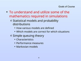
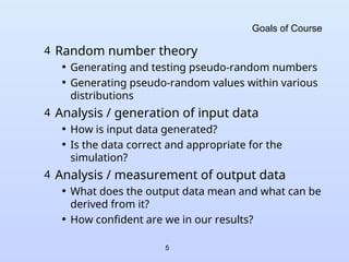

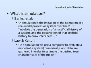
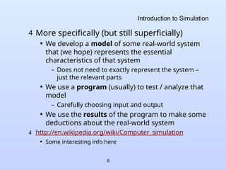
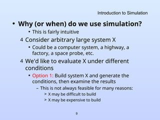


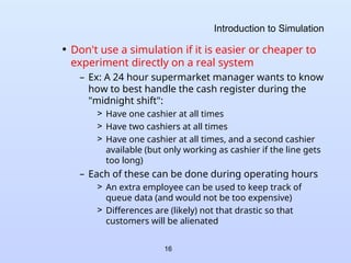
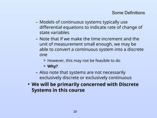
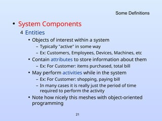
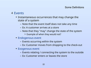
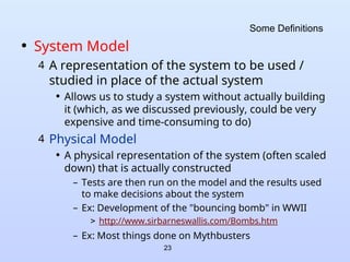
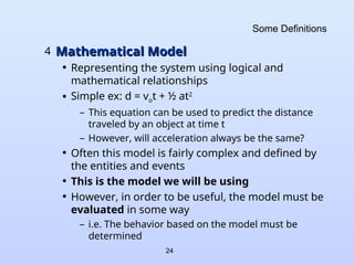
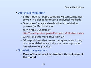
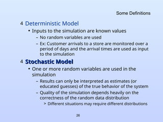
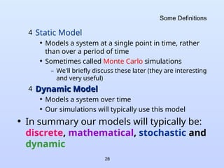
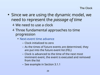
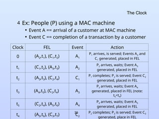
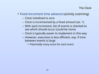
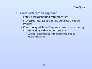
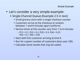
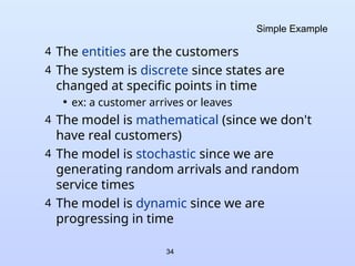
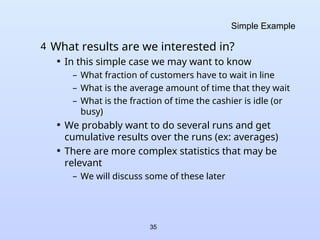
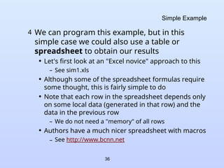
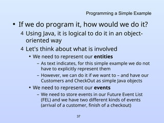
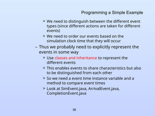
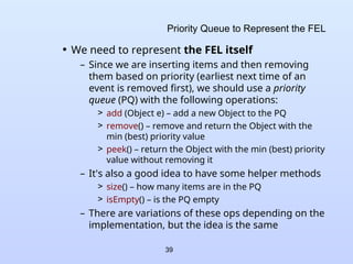

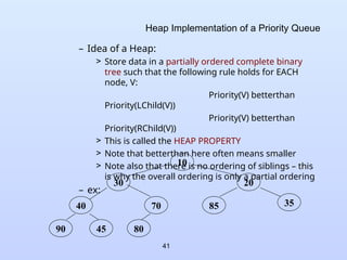
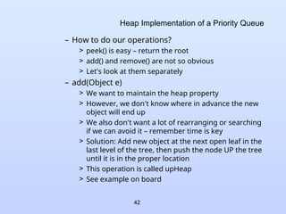
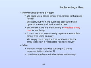
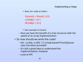


![52
News Dealer's Problem
4 In fact we do we really need to simulate this
problem at all?
• The data is simple and highly mathematical
• Time is not involved
4 Let's try to come up with an analytical solution
to this problem
• We have two distributions, the second of which utilizes
the result of the first
• Let's calculate the expected values for random
variables using these distributions
– For a given discrete random variable X, the expected
value,
E(X) = Sum [xi p(xi)] (more soon in Chapter 5)
all i](https://image.slidesharecdn.com/cs1538-250520024717-b52ecb56/85/Basics-Of-Modeling-And-Simulation-Simulation-Software-52-320.jpg)
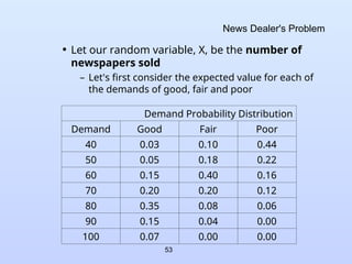
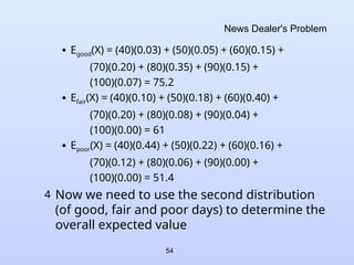
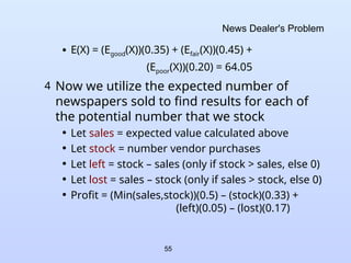

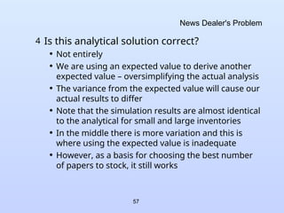
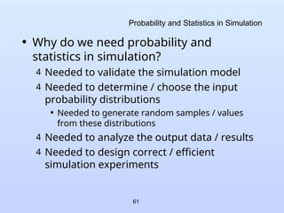
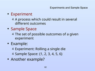
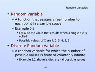
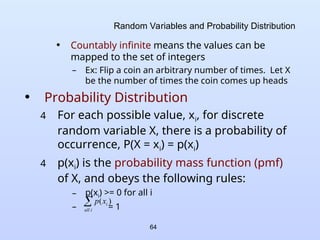
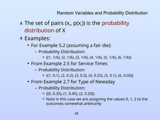
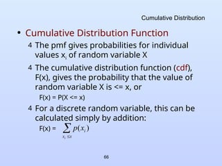
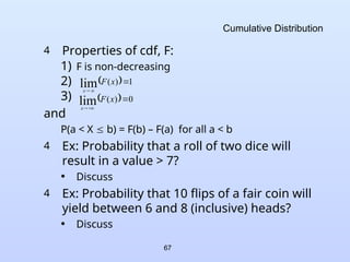
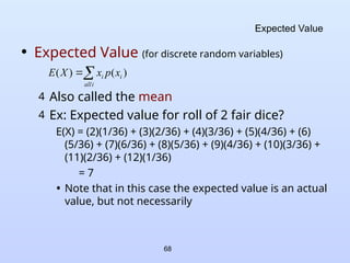
![69
Expected Value and Variance
4 If each value has the same "probability", we
often add the values together and divide by
the number of values to get the mean
(average)
• Ex: Average score on an exam
• Variance
4 We won't prove the identity, but it is useful
]
])
[
[(
)
( 2
X
E
X
E
X
V
)
10
.
5
(
2
2
)]
(
[
)
( Equation
X
E
X
E
](https://image.slidesharecdn.com/cs1538-250520024717-b52ecb56/85/Basics-Of-Modeling-And-Simulation-Simulation-Software-69-320.jpg)
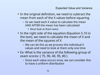
![71
Expected Value and Variance
• V(X) using original definition:
E(X) = (75+90+40+95+80)/5 = 76
V(X) = E[(X – E[X])2
] = [(75-76)2
+ (90-76)2
+ (40-76)2
+ (95-76)2
+ (80-76)2
]/5
= (1 + 196 + 1296 + 361 + 16)/5 =
374
• V(X) using Equation 5.10
E(X) = (75+90+40+95+80)/5 = 76
E(X2
) = (5625+8100+1600+9025+6400)/5 = 6150
V(X) = 6150 – (76)2
= 374
– Note that in this case we can add each number to
one sum and its square to another, so we can
calculate our overall answer with one a single
"look" at each number](https://image.slidesharecdn.com/cs1538-250520024717-b52ecb56/85/Basics-Of-Modeling-And-Simulation-Simulation-Software-71-320.jpg)
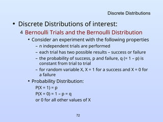
![73
Bernoulli Distribution
• Expected Value
– E(X) = (0)(q) + (1)(p) = p
• Variance
– V(X) = [02
q + 12
p] – p2
= p(1 – p)
4 A single Bernoulli trial is not that interesting
• Typically, multiple trials are performed, from
which we can derive other distributions:
– Binomial Distribution
– Geometric Distribution](https://image.slidesharecdn.com/cs1538-250520024717-b52ecb56/85/Basics-Of-Modeling-And-Simulation-Simulation-Software-73-320.jpg)
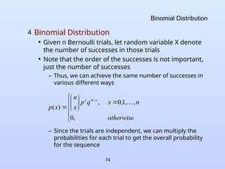
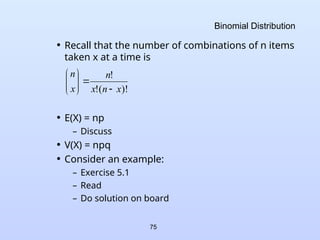

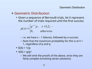
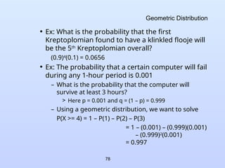
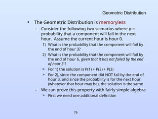
![80
Geometric Distribution
• The conditional probability of an event, A, given
that another event, B, has occurred is defined to
be:
• Applying this to the geometric distribution we get
– Clearly, if X > s+t, then X > s (since t cannot be
negative), so we get
)
(
)
(
)
|
(
B
P
B
A
P
B
A
P
)
(
])
[
]
([
)
|
(
s
X
P
s
X
t
s
X
P
s
X
t
s
X
P
)
(
)
(
)
|
(
s
X
P
t
s
X
P
s
X
t
s
X
P
](https://image.slidesharecdn.com/cs1538-250520024717-b52ecb56/85/Basics-Of-Modeling-And-Simulation-Simulation-Software-80-320.jpg)
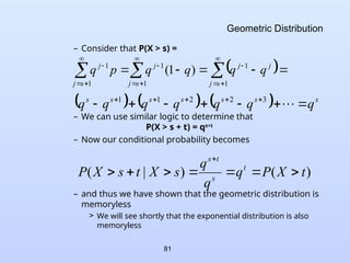
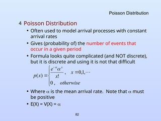
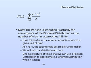
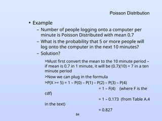
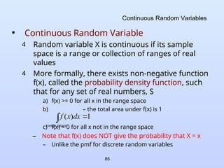
![86
Continuous Random Variables
• The probability that X lies in a given interval [a,b] is
– We see this visually as the "area under the curve"
– Note that for continuous random variables,
P(X = x) = 0 for any x (see from
formula above)
– Rather we always look at the probability of x within a
given range (although the range could be very small)
• The cumulative density function (cdf), F(x) is simply the
integral from - to x or
– This gives us the probability up to x
b
a
dx
x
f
b
X
a
P )
(
)
(
x
dt
t
f
x
F )
(
)
(](https://image.slidesharecdn.com/cs1538-250520024717-b52ecb56/85/Basics-Of-Modeling-And-Simulation-Simulation-Software-86-320.jpg)
![87
Continuous Random Variables
• Ex: Consider the uniform distribution on the range
[a,b] (see text p. 189)
– Look at plots on board for example range [0,1]
> What about F(x) when x < a or x > b?
4 Expected Value for a continuous random variable
– Compare to the discrete expected value
otherwise
b
x
a
if
a
b
x
f
0
1
)
(
x
a
x
a
b
x
a
if
a
b
a
x
dy
a
b
dy
y
f
x
F
1
)
(
)
(
dx
x
xf
X
E )
(
)
(](https://image.slidesharecdn.com/cs1538-250520024717-b52ecb56/85/Basics-Of-Modeling-And-Simulation-Simulation-Software-87-320.jpg)
![88
Continuous Random Variables
4 Variance for continuous random variables
• Defined in same way as for discrete variables
– Calculating it will clearly be different, however
4 Ex: Uniform Distribution
2
)
(
2
)
)(
(
)
(
2
)
(
2
)
(
2
2
2
a
b
a
b
a
b
a
b
a
b
a
b
a
b
x
a
b
dx
a
b
x
X
E
b
a
V(X) = E(X2
) − E(X)
[ ]
2
(Eq 5.10)
=
x2
b − a
dx −
a
b
∫ E(X)
[ ]
2
=
b
a
x3
3(b − a)
−[E(X)]2](https://image.slidesharecdn.com/cs1538-250520024717-b52ecb56/85/Basics-Of-Modeling-And-Simulation-Simulation-Software-88-320.jpg)

(
12
)
(
)
(
3
)
(
12
)
(
4
)
(
4
)
(
)
(
)
(
3
)
(
2
)
)(
(
)
(
3
)
(
2
)
(
3
)]
(
[
)
(
3
)
(
2
3
2
2
3
3
3
2
2
2
2
3
3
3
2
2
3
3
2
3
3
2
2
2
3
3
2
3
3
2
2
2
3
3
2
3
a
b
a
b
a
b
a
b
b
a
ab
a
b
a
b
a
b
a
ab
b
a
ab
b
a
b
a
b
a
b
a
ab
b
a
b
a
b
a
b
a
b
a
b
a
b
a
b
a
b
a
b
a
b
a
b
a
b
a
b
a
b
a
b
a
b
a
b
a
b
a
b
a
b
X
E
a
b
x
a
b
X
V
](https://image.slidesharecdn.com/cs1538-250520024717-b52ecb56/85/Basics-Of-Modeling-And-Simulation-Simulation-Software-89-320.jpg)
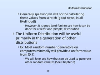
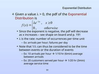
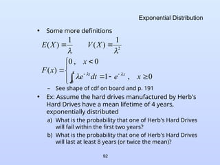
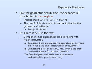
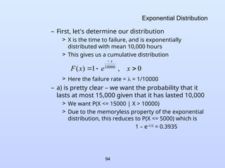
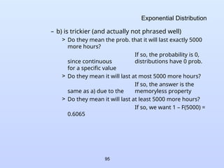
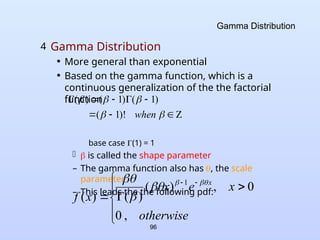
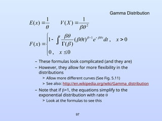
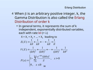
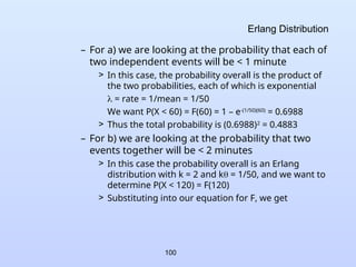
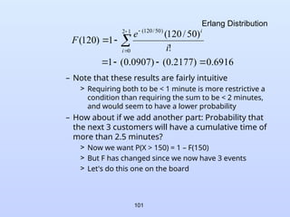
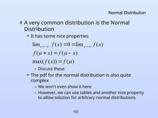
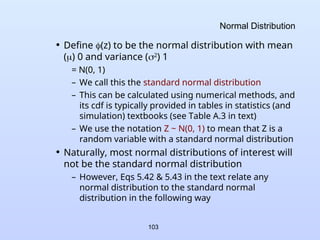
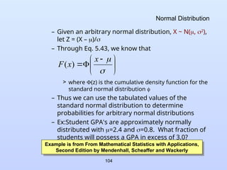
![105
Normal Distribution
– Let Z = (X – 2.4)/0.8
– We want the area under the normal curve with
mean 2.4 and standard deviation 0.8 where x > 3.0
This will be 1 – F(3.0)
F(3.0) = [(3.0 – 2.4)/0.8] = (0.75)
– Looking up (0.75) in Table A.3 we find 0.77337
– Recall that we want 1 – F(3.0), which gives us our
final answer of 1 – 0.77337 = 0.2266
• The idea in general is that we are moving from
the mean in units of standard deviations
– The relationship of the mean to standard deviation
is the same for all normal distributions, which is
why we can use the method indicated](https://image.slidesharecdn.com/cs1538-250520024717-b52ecb56/85/Basics-Of-Modeling-And-Simulation-Simulation-Software-105-320.jpg)
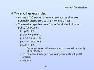
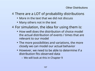
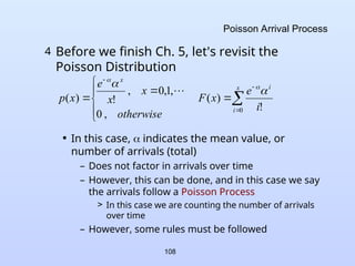
![109
Poisson Arrival Process
1) Arrivals occur one at a time
2) The number of arrivals in a given time period
depends only on the length of that period and not on
the starting point
– i.e. the rate does not change over time
3) The number of arrivals in a given time period does
not affect the number of arrivals in a subsequent
period
– i.e. the number of arrivals in given periods are
independent of each other
– Discuss if these are realistic for actual "arrivals"
• We can alter the Poisson distribution to include
time
– Only difference is that t is substituted for
otherwise
n
n
t
e
n
t
N
P
n
t
,
0
,
1
,
0
,
!
)
(
]
)
(
[
](https://image.slidesharecdn.com/cs1538-250520024717-b52ecb56/85/Basics-Of-Modeling-And-Simulation-Simulation-Software-109-320.jpg)
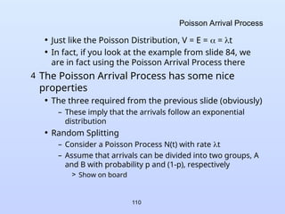
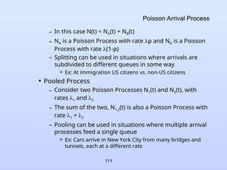
![112
Poisson Arrival Process
• Ex: Exercise 5.28 in text:
– An average of 30 customers per hour arrive at the
Sticky Donut Ship in accordance with a Poisson
process. What is the probability that more than 5
minutes will elapse before both of the next two
customers walk through the door?
> As usual, the first thing is to identify what it is that we
are trying to solve.
> Discuss (and see Notes)
> Note: We could also model this as Erlang Discuss
– [I added this part] If (on average) 75% of Sticky
Donut Shop's customers get their orders to go, what
is the probability that 3 or more new customers will
sit in the dining room in the next 10 minutes?
> Discuss](https://image.slidesharecdn.com/cs1538-250520024717-b52ecb56/85/Basics-Of-Modeling-And-Simulation-Simulation-Software-112-320.jpg)

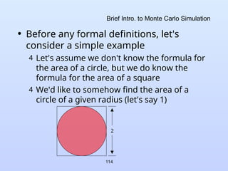

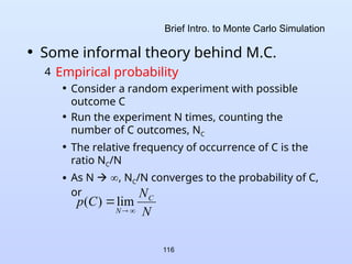
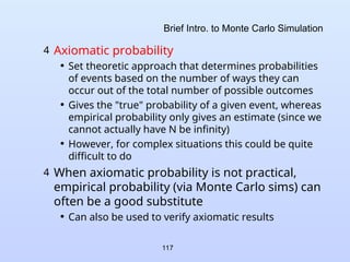
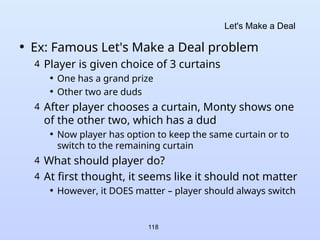
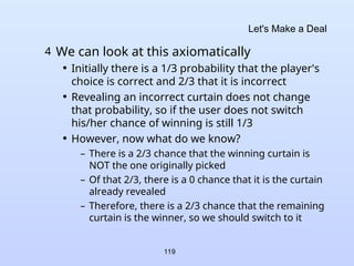


![122
Monte Carlo Integration
4 Consider function f(x) that is defined and
continuous on the range [a,b]
• The first mean value theorem for integral calculus
states that there exists some number c, with a < c <
b such that:
– The idea is that there is some point within the range
(a,b) that is the "average" height of the curve
– So the area of the rectangle with length (b-a) and
height f(c) is the same as the area under the curve
b
a
b
a
c
f
a
b
dx
x
f
or
c
f
dx
x
f
a
b
)
(
)
(
)
(
)
(
)
(
1](https://image.slidesharecdn.com/cs1538-250520024717-b52ecb56/85/Basics-Of-Modeling-And-Simulation-Simulation-Software-122-320.jpg)
![123
Monte Carlo Integration
4 So now all we have to do is determine f(c)
and we can evaluate the integral
4 We can estimate f(c) using Monte Carlo
methods
• Choose N random values x1, … , xN in [a,b]
• Calculate the average (or expected) value, ḟ(x) in
that range:
• Now we can estimate the integral value as
)
(
)
(
1
)
(
1
c
f
x
f
N
x
f
N
i
i
b
a
x
f
a
b
dx
x
f )
(
)
(
)
(](https://image.slidesharecdn.com/cs1538-250520024717-b52ecb56/85/Basics-Of-Modeling-And-Simulation-Simulation-Software-123-320.jpg)
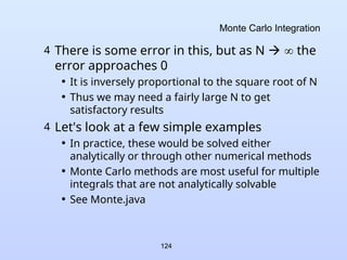
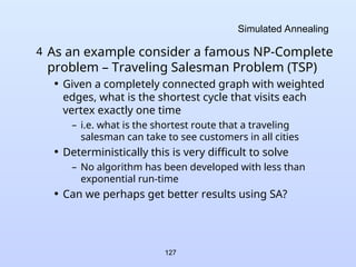
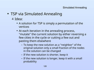
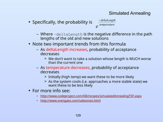
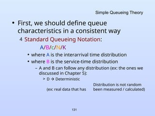
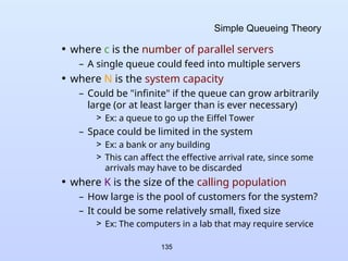
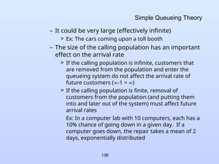
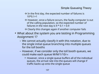
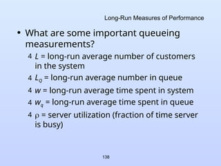
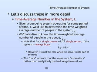
![140
Time-Average Number in System
• We can calculate for an interval [0,T] in a fairly
straightforward manner using a sum:
– Note that each Ti here represents the total time that the
system contained exactly i customers
> These may not be contiguous
– i is shown going to infinity, but in reality most queuing
systems (especially stable queuing systems) will have all
Ti = 0 for i > some value
> In other words, there is some maximum number in the
system that is never exceeded
– See GrocerySimB.java
L
0
1
i
i
T
i
T
L](https://image.slidesharecdn.com/cs1538-250520024717-b52ecb56/85/Basics-Of-Modeling-And-Simulation-Simulation-Software-140-320.jpg)
![141
Time-Average Number in System
4 Let's think of this value in another way:
• Consider the number of customers in the system
at any time, t
– L(t) = number of customers in system at time t
• This value changes as customers enter and leave
the system
• We can graph this with t as the x-axis and L(t) as
the y-axis
• Consider now the area under this plot from [0, T]
– It represents the sum of all of the customers in the
system over all times from [0, T], which can be
determined with an integral
T
dt
t
L
Area
0
)
(](https://image.slidesharecdn.com/cs1538-250520024717-b52ecb56/85/Basics-Of-Modeling-And-Simulation-Simulation-Software-141-320.jpg)
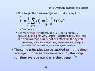
![143
Average Time in System Per Customer
4 Average Time in System Per Customer, w
• This is also a straightforward calculation during our
simulations
– where N is the number of arrivals in the period [0,T]
– where each Wi is the time customer i spends in the
system during the period [0,T]
• If the system is stable, as N , ŵ w
– w is the long-run average system time
• We can do similar calculations for the queue alone to
get the values ŵQ and wQ
– We can think of these values as the observed delay and
the long-run average delay per customer
N
i
i
W
N
w
1
1](https://image.slidesharecdn.com/cs1538-250520024717-b52ecb56/85/Basics-Of-Modeling-And-Simulation-Simulation-Software-143-320.jpg)
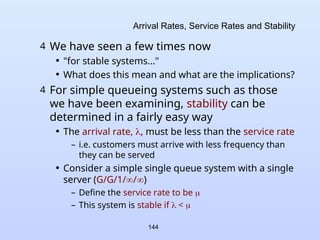
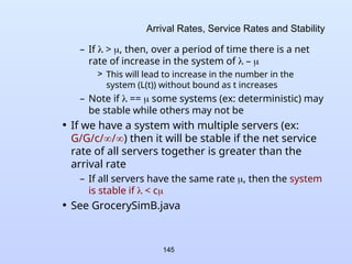
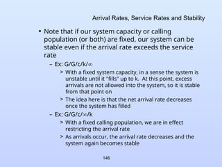
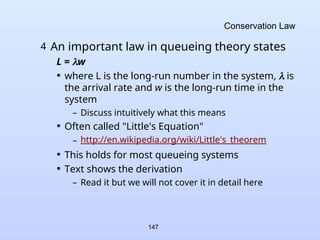
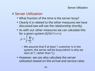
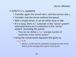
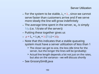
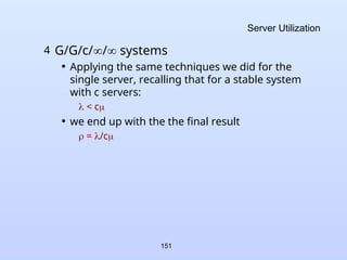

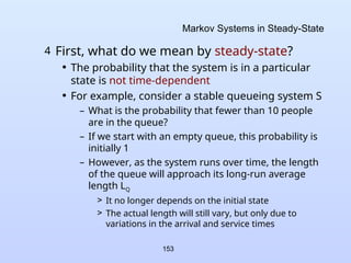
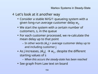
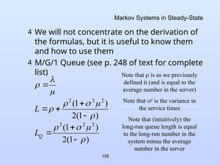
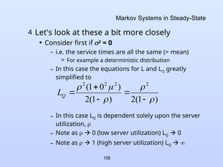
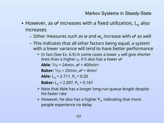
![158
Markov Systems in Steady-State
4 We can generalize this idea, comparing
various distributions using the coefficient of
variation, cv:
(cv)2
= V(X)/[E(X)]2
– i.e. it is the ratio of the variance to the square of
the expected value
• Distributions that have a larger cv have a larger LQ
for a given server utilization, ρ
– In other words, their LQ values increase more
quickly as ρincreases
– Ex: Consider an exponential service distribution:
V(X) = 1/μ2
and E(X) = 1/μ, so (cv)2
= (1/μ)2
/[(1/μ)]2
= 1
> See chart from 4th
Edition of text](https://image.slidesharecdn.com/cs1538-250520024717-b52ecb56/85/Basics-Of-Modeling-And-Simulation-Simulation-Software-158-320.jpg)
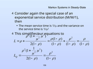
![160
Markov Systems in Steady-State
• The M/M/1 queue gives us a closed form expression
for a measure that the M/G/1 queue does not:
– Pi , the long-run probability that there will be exactly i
customers in the system
– Note: We can use this value to show L for this system
> The last equality is based on the solution to an infinite
geometric series when the base is < 1
> We know ρ < 1 since system must be stable
n
n
P
)
1
(
)
1
1
(
)
1
(
3
3
2
2
0
]
1
[
3
]
1
[
2
]
1
[
1
]
1
[
0
3
2
4
3
3
2
2
3
2
1
0
0
i
i
P
i
L](https://image.slidesharecdn.com/cs1538-250520024717-b52ecb56/85/Basics-Of-Modeling-And-Simulation-Simulation-Software-160-320.jpg)


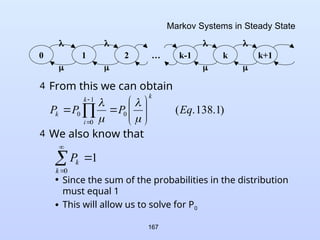
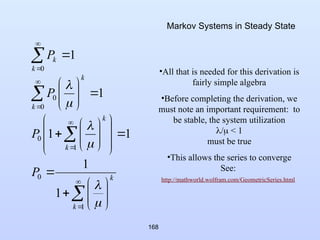
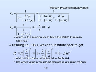

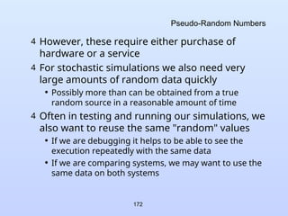
![173
Pseudo-Random Numbers
• Thus, more often than not, simulations rely
on pseudo-random numbers
4 These numbers are generated deterministically
(i.e. can be reproduced)
4 However, they have many (most, we hope) of
the properties of true random numbers:
• Numbers are distributed uniformly on [0,1]
– Assuming a generator from [0,1), which is the most
common
• Numbers should show no correlation with each other
– Must appear to be independent
– There are no discernable patterns in the numbers](https://image.slidesharecdn.com/cs1538-250520024717-b52ecb56/85/Basics-Of-Modeling-And-Simulation-Simulation-Software-173-320.jpg)
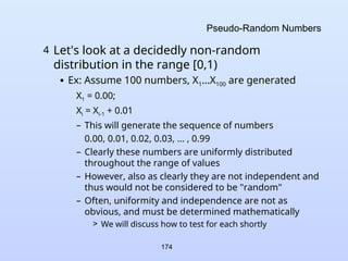
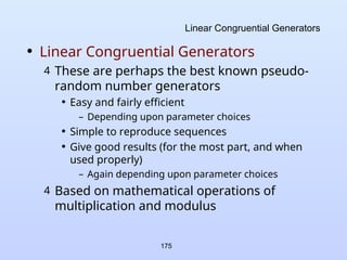
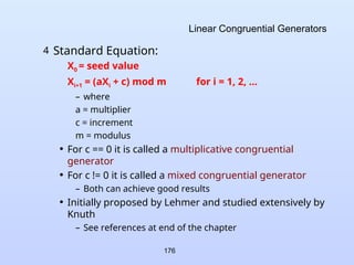

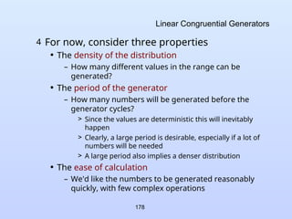
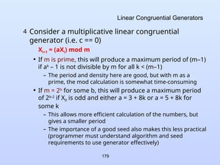
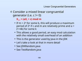

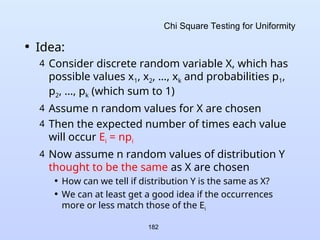
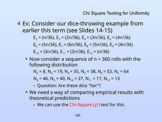
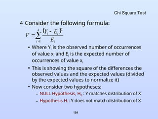
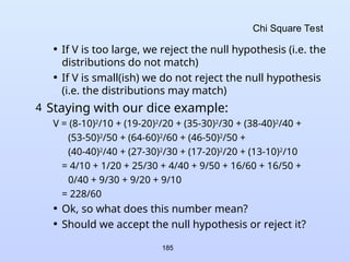
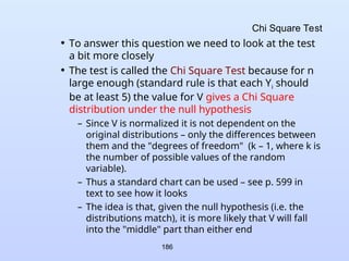
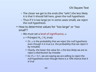
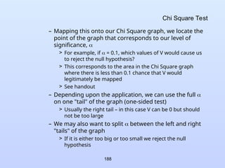
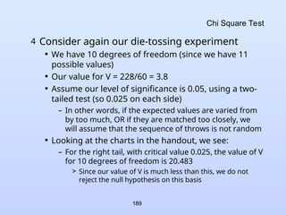
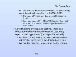

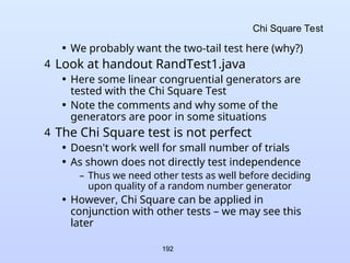

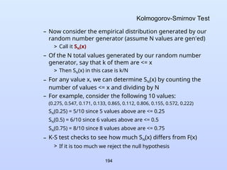
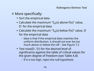
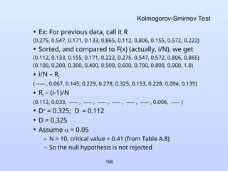

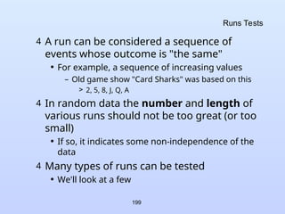
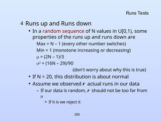
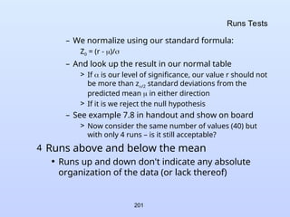
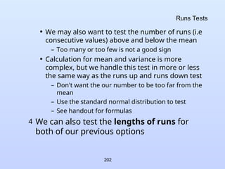
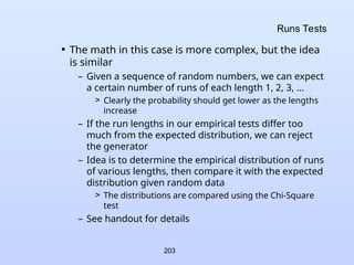
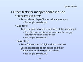
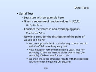
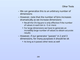
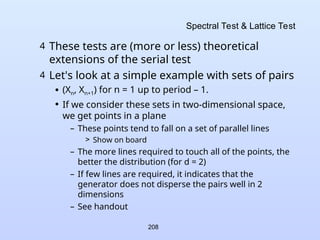

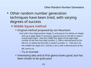
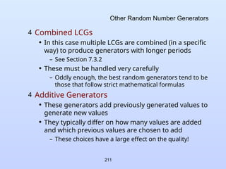
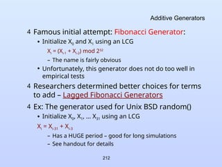
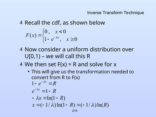
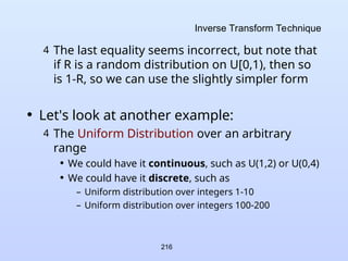
![217
Uniform Distributions on Different Ranges
• Continuous uniform distributions
– Given R U[0,1), we may need to do 2 different
things to get an arbitrary uniform distribution
> Expand (or compress) the range to be larger (or
smaller)
> Shift it to get a different starting point
– The text shows a derivation of the formula, but we
can do it intuitively, based on the two goals above
> To expand the range we need to multiply R by the
length of the range desired
> To get the correct starting point, we need to add (to
0) the starting point we want
– Consider the desired range [a,b]. Our
transformations yield
X = a + (b – a)R](https://image.slidesharecdn.com/cs1538-250520024717-b52ecb56/85/Basics-Of-Modeling-And-Simulation-Simulation-Software-217-320.jpg)
![218
Uniform Distributions on Different Ranges
• Discrete uniform distributions
– The formula in this case is quite similar to that for
the continuous case
– However, care must be paid to the range and any
error due to truncation
– Consider a discrete uniform range [m, n] for
integers m, m+1, … , n-1, n
– If we use
X = m + (n – m)R
> The minimum value is correct, since the minimum
result for X is m (since R can be 0)
> Now we need to be sure of two things:
1) The maximum value is correct
2) The probabilities of all values are the same](https://image.slidesharecdn.com/cs1538-250520024717-b52ecb56/85/Basics-Of-Modeling-And-Simulation-Simulation-Software-218-320.jpg)
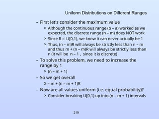
![220
Uniform Distributions on Different Ranges
• Each sub-interval is equal in range and thus has
equal probability
• Given R in each sub-interval, a distinct value in the
range [m,n] will result
– Ex: Assume R is in the second sub-interval above
– We then have
m + (n – m + 1)(1/(n – m + 1)) = m + 1 X <
m + (n – m + 1)(2/(n – m + 1)) = m + 2
– Since X is an integer, and is strictly less than m + 2,
the entire sub-interval maps into m + 1
1
1
,
1
1
2
,
1
1
,
1
1
,
0
m
n
m
n
m
n
m
n
m
n
m
n
m
n
](https://image.slidesharecdn.com/cs1538-250520024717-b52ecb56/85/Basics-Of-Modeling-And-Simulation-Simulation-Software-220-320.jpg)
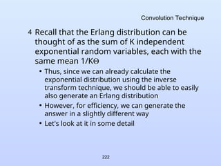
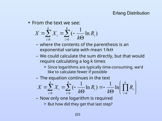

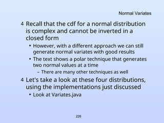


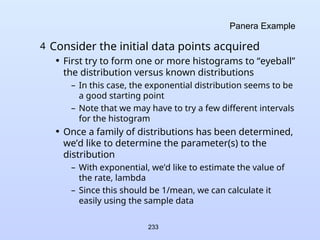

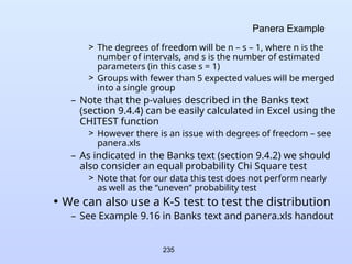
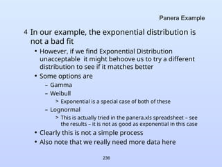
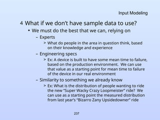
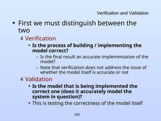
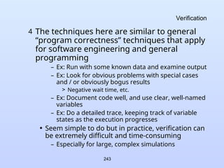
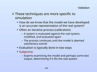
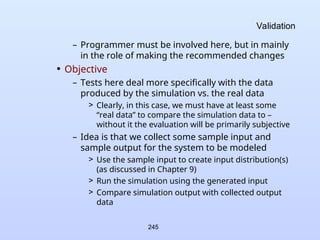
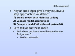
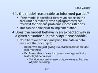
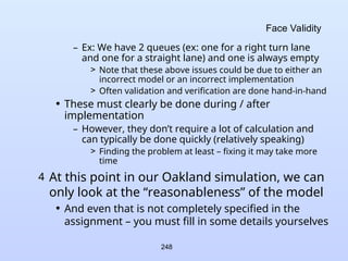
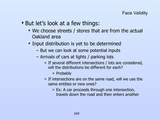
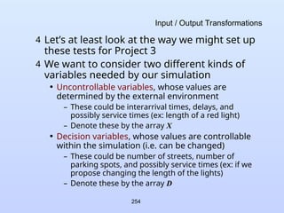
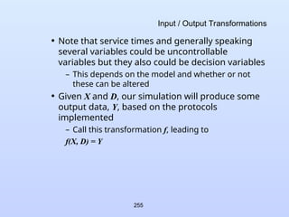
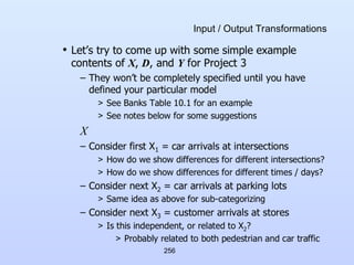
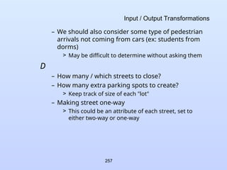
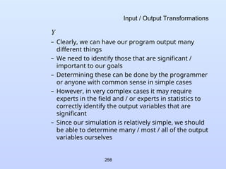
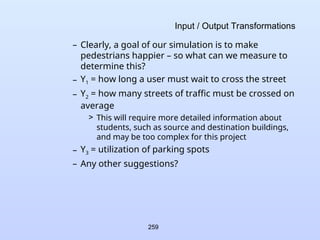
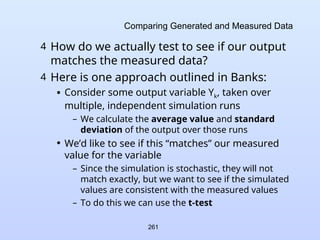
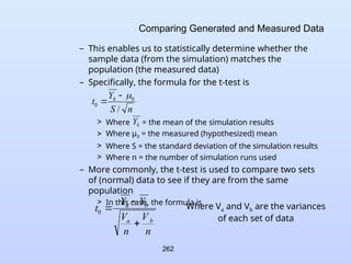
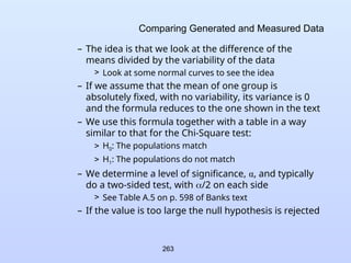
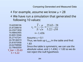
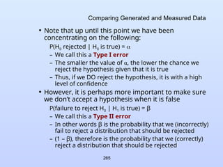
![266
Comparing Generated and Measured Data
– We call (1 – β) the power of the test, and clearly a
high value for (1 – β) [equal to a low value for β] is
desirable
– Unfortunately, for a given value of , the only way
to increase the power of the test (i.e. reduce Type II
error) is to increase the number of points, n
– See ttest.xls for more info
• The existence of Type II errors is why we are
cautious with our Type I error test:
– “We fail to reject the null hypothesis”
– This is also why we looked at the p-values in
Chapter 9 when discussing distribution fits
– The better the fit, the higher the p-value and the
lower the chance of Type II errors](https://image.slidesharecdn.com/cs1538-250520024717-b52ecb56/85/Basics-Of-Modeling-And-Simulation-Simulation-Software-266-320.jpg)
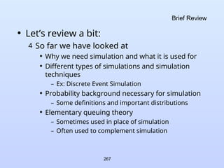
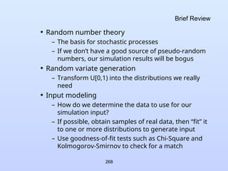
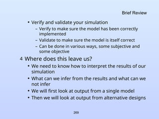
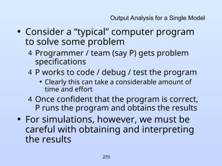
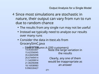
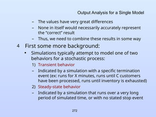
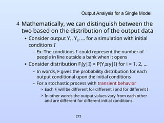
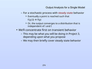
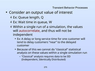
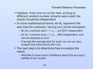
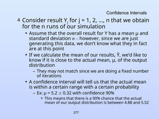
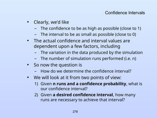
![279
Confidence Intervals
4 Let’s first look at 1) Given n runs and a
confidence probability, what is our
confidence interval?
• First, we determine the point estimate, Ῡ, for our
distribution
– This is simply
> The mean of the sample points (Equation 11.1)
• We next need to determine the sample variance,
S2
n
Y
n
j
j
1
1
2
1
2
2
n
Y
n
Y
S
n
j
j
Note: This is the variance formula
E(X2
)-[E(X)]2
formula, except that it is dividing by n-
1 rather than n, which makes it an
unbiased estimator of the population
variance (see this link)](https://image.slidesharecdn.com/cs1538-250520024717-b52ecb56/85/Basics-Of-Modeling-And-Simulation-Simulation-Software-279-320.jpg)
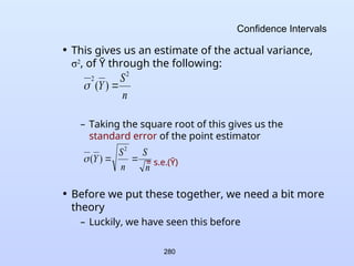
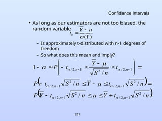
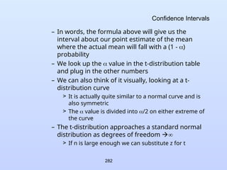
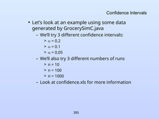
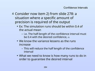
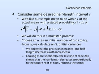
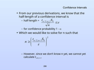
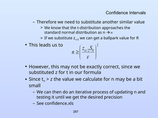
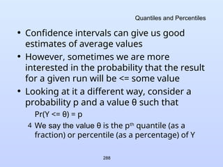
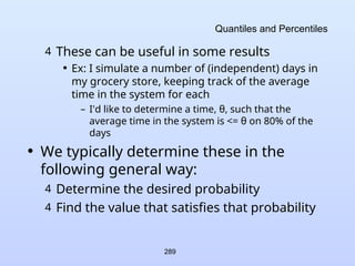
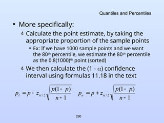
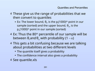
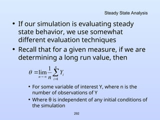

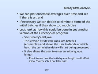
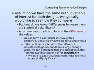
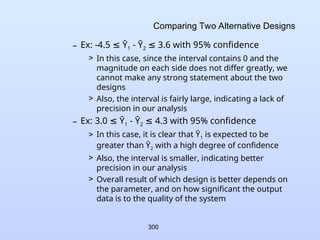
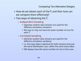
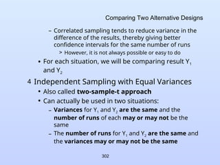
![303
Comparing Two Alternative Designs
4 First recall what it is that we want to calculate:
• The confidence interval of the difference of the two
results, or
(Ῡ.1 - Ῡ.2) ± t/2,v [s.e.(Ῡ.1 - Ῡ.2)] with prob. (1-)
– To calculate this we need to determine the standard
error for the difference of the two means, and the
degrees of freedom, v
• Consider Ῡ.1 - Ῡ.2 and, more specifically the variance
of Ῡ.1 - Ῡ.2
• Since the runs are independent
Var(Ῡ.1 - Ῡ.2) = Var(Ῡ.1) + Var(Ῡ.2)
= σ1
2
/R1 + σ2
2
/R2](https://image.slidesharecdn.com/cs1538-250520024717-b52ecb56/85/Basics-Of-Modeling-And-Simulation-Simulation-Software-303-320.jpg)
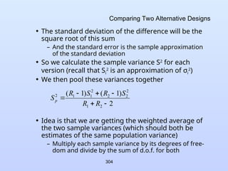
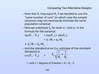

![308
Comparing Two Alternative Designs
• Because the true variances differ, we cannot pool
the sample variances, and must calculate the
standard error using the following equation
• The degrees of freedom is then estimated by
– This technique is actually very old, developed by
Welch in 1938 and discussed [Scheffe, 1970]
2
2
2
1
2
1
2
1
2
1 )
var(
)
var(
)
.(
.
R
S
R
S
Y
Y
Y
Y
e
s
)]
1
/(
)
/
[(
)]
1
/(
)
/
[(
)
/
/
(
2
2
2
2
2
1
2
1
2
1
2
2
2
2
1
2
1
R
R
S
R
R
S
R
S
R
S
v](https://image.slidesharecdn.com/cs1538-250520024717-b52ecb56/85/Basics-Of-Modeling-And-Simulation-Simulation-Software-308-320.jpg)
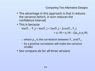

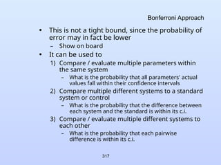
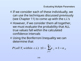
![322
Comparing Multiple Systems Pairwise
• As mentioned previously, in this case we
have K(K-1)/2 pairs for K different systems
4 We look for differences pairwise, just as in the
previous technique
4 However, now we have a lot more pairs to
consider and therefore the individual
probabilities must be a lot higher
• This can present a problem for even a moderate K
• Ex: = 0.1, K = 5
– Each i must be (0.1)/[(5)(4)/2] = 0.01
• Again, this will create either very large intervals or
require a large number of runs](https://image.slidesharecdn.com/cs1538-250520024717-b52ecb56/85/Basics-Of-Modeling-And-Simulation-Simulation-Software-322-320.jpg)