SlideShare a Scribd company logo
1 of 7
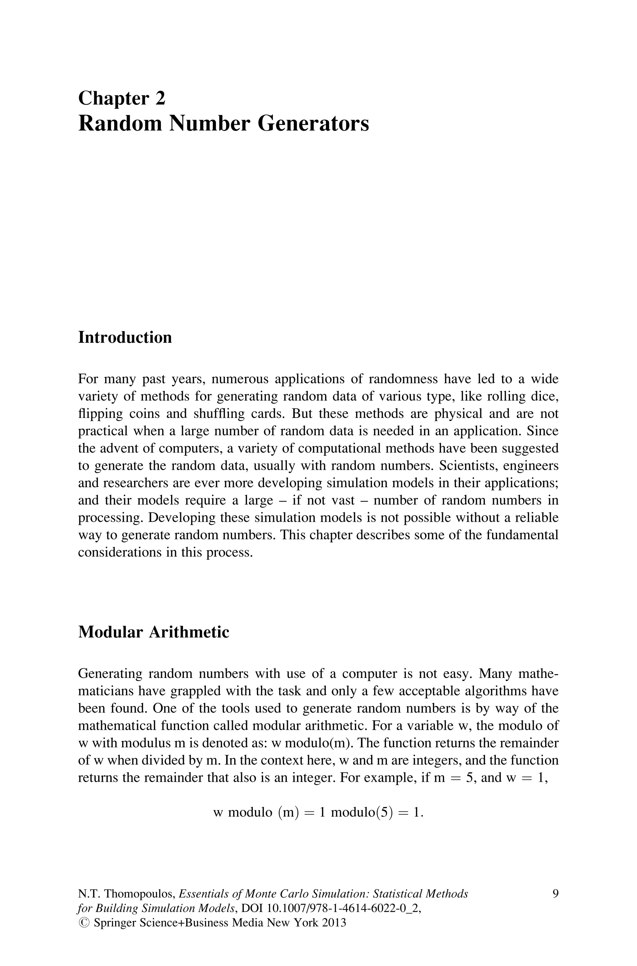
Chapter 2
Random Number Generators


Introduction

For many past years, numerous applications of randomness have led to a wide
variety of methods for generating random data of various type, like rolling dice,
flipping coins and shuffling cards. But these methods are physical and are not
practical when a large number of random data is needed in an application. Since
the advent of computers, a variety of computational methods have been suggested
to generate the random data, usually with random numbers. Scientists, engineers
and researchers are ever more developing simulation models in their applications;
and their models require a large – if not vast – number of random numbers in
processing. Developing these simulation models is not possible without a reliable
way to generate random numbers. This chapter describes some of the fundamental
considerations in this process.


Modular Arithmetic

Generating random numbers with use of a computer is not easy. Many mathe-
maticians have grappled with the task and only a few acceptable algorithms have
been found. One of the tools used to generate random numbers is by way of the
mathematical function called modular arithmetic. For a variable w, the modulo of
w with modulus m is denoted as: w modulo(m). The function returns the remainder
of w when divided by m. In the context here, w and m are integers, and the function
returns the remainder that also is an integer. For example, if m ¼ 5, and w ¼ 1,

                         w modulo ðmÞ ¼ 1 moduloð5Þ ¼ 1:


N.T. Thomopoulos, Essentials of Monte Carlo Simulation: Statistical Methods      9
for Building Simulation Models, DOI 10.1007/978-1-4614-6022-0_2,
# Springer Science+Business Media New York 2013
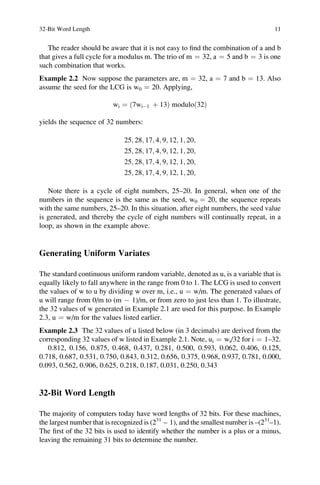
10                                                      2 Random Number Generators


     In the same way, should w ¼ 5, 6 or 17, then,

                                  5 moduloð5Þ ¼ 0
                                  6 moduloð5Þ ¼ 1
                                 17 moduloð5Þ ¼ 2

and so forth. Hence, for example, the numbers 1, 6, 11, 16 are all congruent
modulo 1 when m ¼ 5. Note, the difference of any of the numbers, that have the
same remainder, is perfectly divisible by m, and thus they are congruent. Also
notice, when the parameter is m, the values returned are all integers, 0 to m-1.
   An example of modular arithmetic is somewhat like the clock where the
numbers for the hours are always from 1 to 12. The same applies with the days of
the week (1–7), and the months of the year (1–12).


Linear Congruent Generators

In 1951, Lehmer introduced a way to generated random numbers, called the linear
congruent generator, LCG. This method adapts well to computer applications and
today is the most common technique in use. The method requires the use of the
modulo function as shown below.
   LCG calls for three parameters (a, b, m) and uses modular arithmetic. To obtain
the i-th value of w, the function uses the prior value of w as in the method
shown below:

                           wi ¼ ða wiÀ1 þ bÞ moduloðmÞ

   In the above, w is a sequence of integers that are generated from this function,
and i is the index of the sequence.
Example 2.1 Suppose, m ¼ 32, a ¼ 5 and b ¼ 3. Also, assume the seed (at i ¼ 0)
for the LCG is w0 ¼ 11. Applying,

                           wi ¼ ð5wiÀ1 þ 3Þ moduloð32Þ

yields the sequence:
   26,5,28,15,14,9,16,19,2,13,4,23,22,17,24,27,10,21,12,31,30,25,0,3,18,29,20,7,
6,1,8,11
   Notice there are 32 values of w for i ranging from 1 to 32, and all are different.
This is called a full cycle of all the possible remainders 0–31 when m ¼ 32. The last
number in the sequence is the same as the seed, w0 ¼ 11. The sequence of numbers
that are generated for the second cycle would be the same as the sequence from the
first cycle of 32 numbers because the seed has been repeated.
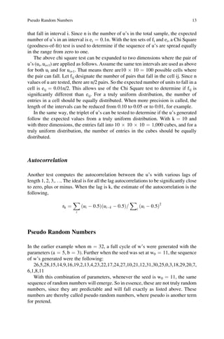
32-Bit Word Length                                                                   11


   The reader should be aware that it is not easy to find the combination of a and b
that gives a full cycle for a modulus m. The trio of m ¼ 32, a ¼ 5 and b ¼ 3 is one
such combination that works.
Example 2.2 Now suppose the parameters are, m ¼ 32, a ¼ 7 and b ¼ 13. Also
assume the seed for the LCG is w0 ¼ 20. Applying,

                          wi ¼ ð7wiÀ1 þ 13Þ moduloð32Þ

yields the sequence of 32 numbers:

                              25; 28; 17; 4; 9; 12; 1; 20;
                              25; 28; 17; 4; 9; 12; 1; 20;
                              25; 28; 17; 4; 9; 12; 1; 20;
                              25; 28; 17; 4; 9; 12; 1; 20;

   Note there is a cycle of eight numbers, 25–20. In general, when one of the
numbers in the sequence is the same as the seed, w0 ¼ 20, the sequence repeats
with the same numbers, 25–20. In this situation, after eight numbers, the seed value
is generated, and thereby the cycle of eight numbers will continually repeat, in a
loop, as shown in the example above.


Generating Uniform Variates

The standard continuous uniform random variable, denoted as u, is a variable that is
equally likely to fall anywhere in the range from 0 to 1. The LCG is used to convert
the values of w to u by dividing w over m, i.e., u ¼ w/m. The generated values of
u will range from 0/m to (m À 1)/m, or from zero to just less than 1. To illustrate,
the 32 values of w generated in Example 2.1 are used for this purpose. In Example
2.3, u ¼ w/m for the values listed earlier.
Example 2.3 The 32 values of u listed below (in 3 decimals) are derived from the
corresponding 32 values of w listed in Example 2.1. Note, ui ¼ wi/32 for i ¼ 1–32.
   0.812, 0.156, 0.875, 0.468, 0.437, 0.281, 0.500, 0.593, 0.062, 0.406, 0.125,
0.718, 0.687, 0.531, 0.750, 0.843, 0.312, 0.656, 0.375, 0.968, 0.937, 0.781, 0.000,
0.093, 0.562, 0.906, 0.625, 0.218, 0.187, 0.031, 0.250, 0.343


32-Bit Word Length

The majority of computers today have word lengths of 32 bits. For these machines,
the largest number that is recognized is (231 – 1), and the smallest number is –(231–1).
The first of the 32 bits is used to identify whether the number is a plus or a minus,
leaving the remaining 31 bits to determine the number.
12                                                       2 Random Number Generators


   So, for these machines, the ideal value of the modulus is m ¼ (231–1) since a full
cycle with m gives a sequence with the largest number of unique random uniform
variables The goal is to find a combination of parameters that are compatible with
the modulus. Fishman and Moore (1982), have done extensive analysis on random
number generators determining their acceptability for simulation use. In 1969,
Lewis, Goodman and Miller suggested the parameter values of a ¼ 16,807 and
b ¼ 0; and also in 1969, Payne, Rabung and Bogyo offered a ¼ 630,360,016 with
b ¼ 0. These combinations have been installed in computer compilers and are
accepted as parameter combinations that are acceptable for scientific use. The Fishman
and Moore reference also identifies other multipliers that achieve good results.


Random Number Generator Tests

Mathematicians have developed a series of tests to evaluate how good a sequence of
uniform variates are with respect to truly random uniform variates. Some of the
tests are described below.


Length of the Cycle

The first consideration is how many variates are generated before the cycle repeats.
The most important rule is to have a full cycle with the length of the modulus m.
Assume that n uniform variates are generated and are labeled as (u1, . . ., un) where
n ¼ m or is close to m. The ideal would be to generate random numbers where the
numbers span a full cycle or very near a full cycle.


Mean and Variance

For the set of n variates (u1, . . ., un), the sample average and variance are computed
                 
and labeled as u and su2, respectively. The goal of the random number generator
is to emulate the standard continuous uniform random variable u, denoted here
as u ~ U(0,1), with expected value E(u) ¼ 0.5 and the variance V(u) ¼ s2 ¼ 1/12 ¼
0.0833. So, the appropriate hypothesis mean and variance tests are used to compare

u to 0.5 and su2 to 0.0833.


Chi Square

The sequence (u1, . . ., un) are set in k intervals, say k ¼ 10, where i ¼ 1–10
identifies the interval for which each u falls. When k ¼ 10, the intervals are:
(0.0–0.1), (0.1–0.2), . . .., (0.9–1.0). Now let fi designate the number of u’s
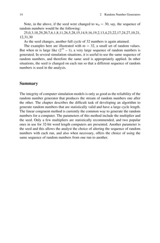
Pseudo Random Numbers                                                                    13


that fall in interval i. Since n is the number of u’s in the total sample, the expected
number of u’s in an interval is ei ¼ 0.1n. With the ten sets of fi and ei, a Chi Square
(goodness-of-fit) test is used to determine if the sequence of u’s are spread equally
in the range from zero to one.
   The above chi square test can be expanded to two dimensions where the pair of
u’s (ui, ui+1) are applied as follows. Assume the same ten intervals are used as above
for both ui and for ui+1. That means there are10 Â 10 ¼ 100 possible cells where
the pair can fall. Let fij designate the number of pairs that fall in the cell ij. Since n
values of u are tested, there are n/2 pairs. So the expected number of units to fall in a
cell is eij ¼ 0.01n/2. This allows use of the Chi Square test to determine if fij is
significantly different than eij. For a truly uniform distribution, the number of
entries in a cell should be equally distributed. When more precision is called, the
length of the intervals can be reduced from 0.10 to 0.05 or to 0.01, for example.
   In the same way, the triplet of u’s can be tested to determine if the u’s generated
follow the expected values from a truly uniform distribution. With k ¼ 10 and
with three dimensions, the entries fall into 10 Â 10 Â 10 ¼ 1,000 cubes, and for a
truly uniform distribution, the number of entries in the cubes should be equally
distributed.


Autocorrelation

Another test computes the autocorrelation between the u’s with various lags of
length 1, 2, 3,. . .. The ideal is for all the lag autocorrelations to be significantly close
to zero, plus or minus. When the lag is k, the estimate of the autocorrelation is the
following,
                          X                             X
                   rk ¼       ðui À 0:5ÞðuiÀk À 0:5Þ=      i
                                                               ðui À 0:5Þ2
                          i


Pseudo Random Numbers

In the earlier example when m ¼ 32, a full cycle of w’s were generated with the
parameters (a ¼ 5, b ¼ 3). Further when the seed was set at w0 ¼ 11, the sequence
of w’s generated were the following:
   26,5,28,15,14,9,16,19,2,13,4,23,22,17,24,27,10,21,12,31,30,25,0,3,18,29,20,7,
6,1,8,11
   With this combination of parameters, whenever the seed is w0 ¼ 11, the same
sequence of random numbers will emerge. So in essence, these are not truly random
numbers, since they are predictable and will fall exactly as listed above. These
numbers are thereby called pseudo random numbers, where pseudo is another term
for pretend.
14                                                      2 Random Number Generators


    Note, in the above, if the seed were changed to w0 ¼ 30, say, the sequence of
random numbers would be the following:
    25,0,3,18,29,20,7,6,1,8,11,26,5,28,15,14,9,16,19,2,13,4,23,22,17,24,27,10,21,
12,31,30
    As the seed changes, another full cycle of 32 numbers is again attained.
    The examples here are illustrated with m ¼ 32, a small set of random values.
But when m is large like (231 – 1), a very large sequence of random numbers is
generated. In several simulation situations, it is useful to use the same sequence of
random numbers, and therefore the same seed is appropriately applied. In other
situations, the seed is changed on each run so that a different sequence of random
numbers is used in the analysis.


Summary

The integrity of computer simulation models is only as good as the reliability of the
random number generator that produces the stream of random numbers one after
the other. The chapter describes the difficult task of developing an algorithm to
generate random numbers that are statistically valid and have a large cycle length.
The linear congruent method is currently the common way to generate the random
numbers for a computer. The parameters of this method include the multiplier and
the seed. Only a few multipliers are statistically recommended, and two popular
ones in use for 32-bit word length computers are presented. Another parameter is
the seed and this allows the analyst the choice of altering the sequence of random
numbers with each run, and also when necessary, offers the choice of using the
same sequence of random numbers from one run to another.
http://www.springer.com/978-1-4614-6021-3

More Related Content

What's hot

A Monte Carlo strategy for structure multiple-step-head time series prediction
A Monte Carlo strategy for structure multiple-step-head time series predictionA Monte Carlo strategy for structure multiple-step-head time series prediction
A Monte Carlo strategy for structure multiple-step-head time series predictionGianluca Bontempi
 
Predicting Stock Market Price Using Support Vector Regression
Predicting Stock Market Price Using Support Vector RegressionPredicting Stock Market Price Using Support Vector Regression
Predicting Stock Market Price Using Support Vector RegressionChittagong Independent University
 
Types of Mathematical Model.
Types of Mathematical Model.Types of Mathematical Model.
Types of Mathematical Model.Megha Sharma
 
A Novel Methodology to Implement Optimization Algorithms in Machine Learning
A Novel Methodology to Implement Optimization Algorithms in Machine LearningA Novel Methodology to Implement Optimization Algorithms in Machine Learning
A Novel Methodology to Implement Optimization Algorithms in Machine LearningVenkata Karthik Gullapalli
 
Computational Intelligence for Time Series Prediction
Computational Intelligence for Time Series PredictionComputational Intelligence for Time Series Prediction
Computational Intelligence for Time Series PredictionGianluca Bontempi
 
Lecture 2: Preliminaries (Understanding and Preprocessing data)
Lecture 2: Preliminaries (Understanding and Preprocessing data)Lecture 2: Preliminaries (Understanding and Preprocessing data)
Lecture 2: Preliminaries (Understanding and Preprocessing data)Marina Santini
 
Operational Research
Operational ResearchOperational Research
Operational ResearchRoy Thomas
 
Computer simulation technique the definitive introduction - harry perros
Computer simulation technique   the definitive introduction - harry perrosComputer simulation technique   the definitive introduction - harry perros
Computer simulation technique the definitive introduction - harry perrosJesmin Rahaman
 
2. System Simulation modeling unit i
2. System Simulation modeling unit i2. System Simulation modeling unit i
2. System Simulation modeling unit iAmita Gautam
 
Applications of simulation in Business with Example
Applications of simulation in Business with ExampleApplications of simulation in Business with Example
Applications of simulation in Business with ExamplePratima Ray
 
Classification Based Machine Learning Algorithms
Classification Based Machine Learning AlgorithmsClassification Based Machine Learning Algorithms
Classification Based Machine Learning AlgorithmsMd. Main Uddin Rony
 
Local modeling in regression and time series prediction
Local modeling in regression and time series predictionLocal modeling in regression and time series prediction
Local modeling in regression and time series predictionGianluca Bontempi
 
Lecture 9: Machine Learning in Practice (2)
Lecture 9: Machine Learning in Practice (2)Lecture 9: Machine Learning in Practice (2)
Lecture 9: Machine Learning in Practice (2)Marina Santini
 
Machine Learning Unit 3 Semester 3 MSc IT Part 2 Mumbai University
Machine Learning Unit 3 Semester 3  MSc IT Part 2 Mumbai UniversityMachine Learning Unit 3 Semester 3  MSc IT Part 2 Mumbai University
Machine Learning Unit 3 Semester 3 MSc IT Part 2 Mumbai UniversityMadhav Mishra
 
Feature selection concepts and methods
Feature selection concepts and methodsFeature selection concepts and methods
Feature selection concepts and methodsReza Ramezani
 

What's hot (17)

Conceptual modeling
Conceptual modelingConceptual modeling
Conceptual modeling
 
A Monte Carlo strategy for structure multiple-step-head time series prediction
A Monte Carlo strategy for structure multiple-step-head time series predictionA Monte Carlo strategy for structure multiple-step-head time series prediction
A Monte Carlo strategy for structure multiple-step-head time series prediction
 
Predicting Stock Market Price Using Support Vector Regression
Predicting Stock Market Price Using Support Vector RegressionPredicting Stock Market Price Using Support Vector Regression
Predicting Stock Market Price Using Support Vector Regression
 
Types of Mathematical Model.
Types of Mathematical Model.Types of Mathematical Model.
Types of Mathematical Model.
 
A Novel Methodology to Implement Optimization Algorithms in Machine Learning
A Novel Methodology to Implement Optimization Algorithms in Machine LearningA Novel Methodology to Implement Optimization Algorithms in Machine Learning
A Novel Methodology to Implement Optimization Algorithms in Machine Learning
 
Computational Intelligence for Time Series Prediction
Computational Intelligence for Time Series PredictionComputational Intelligence for Time Series Prediction
Computational Intelligence for Time Series Prediction
 
Lecture 2: Preliminaries (Understanding and Preprocessing data)
Lecture 2: Preliminaries (Understanding and Preprocessing data)Lecture 2: Preliminaries (Understanding and Preprocessing data)
Lecture 2: Preliminaries (Understanding and Preprocessing data)
 
Operational Research
Operational ResearchOperational Research
Operational Research
 
Computer simulation technique the definitive introduction - harry perros
Computer simulation technique   the definitive introduction - harry perrosComputer simulation technique   the definitive introduction - harry perros
Computer simulation technique the definitive introduction - harry perros
 
2. System Simulation modeling unit i
2. System Simulation modeling unit i2. System Simulation modeling unit i
2. System Simulation modeling unit i
 
Applications of simulation in Business with Example
Applications of simulation in Business with ExampleApplications of simulation in Business with Example
Applications of simulation in Business with Example
 
Classification Based Machine Learning Algorithms
Classification Based Machine Learning AlgorithmsClassification Based Machine Learning Algorithms
Classification Based Machine Learning Algorithms
 
Local modeling in regression and time series prediction
Local modeling in regression and time series predictionLocal modeling in regression and time series prediction
Local modeling in regression and time series prediction
 
Lecture 9: Machine Learning in Practice (2)
Lecture 9: Machine Learning in Practice (2)Lecture 9: Machine Learning in Practice (2)
Lecture 9: Machine Learning in Practice (2)
 
Simulation Software Performances And Examples
Simulation Software Performances And ExamplesSimulation Software Performances And Examples
Simulation Software Performances And Examples
 
Machine Learning Unit 3 Semester 3 MSc IT Part 2 Mumbai University
Machine Learning Unit 3 Semester 3  MSc IT Part 2 Mumbai UniversityMachine Learning Unit 3 Semester 3  MSc IT Part 2 Mumbai University
Machine Learning Unit 3 Semester 3 MSc IT Part 2 Mumbai University
 
Feature selection concepts and methods
Feature selection concepts and methodsFeature selection concepts and methods
Feature selection concepts and methods
 

Similar to Essentials of monte carlo simulation

A Study on Differential Equations on the Sphere Using Leapfrog Method
A Study on Differential Equations on the Sphere Using Leapfrog MethodA Study on Differential Equations on the Sphere Using Leapfrog Method
A Study on Differential Equations on the Sphere Using Leapfrog Methodiosrjce
 
Prime Number Validator
Prime Number ValidatorPrime Number Validator
Prime Number ValidatorMohammad Hefny
 
IRJET- An Efficient Reverse Converter for the Three Non-Coprime Moduli Set {4...
IRJET- An Efficient Reverse Converter for the Three Non-Coprime Moduli Set {4...IRJET- An Efficient Reverse Converter for the Three Non-Coprime Moduli Set {4...
IRJET- An Efficient Reverse Converter for the Three Non-Coprime Moduli Set {4...IRJET Journal
 
161783709 chapter-04-answers
161783709 chapter-04-answers161783709 chapter-04-answers
161783709 chapter-04-answersBookStoreLib
 
161783709 chapter-04-answers
161783709 chapter-04-answers161783709 chapter-04-answers
161783709 chapter-04-answersFiras Husseini
 
Bender’s Decomposition Method for a Large Two-stage Linear Programming Model
Bender’s Decomposition Method for a Large Two-stage Linear Programming ModelBender’s Decomposition Method for a Large Two-stage Linear Programming Model
Bender’s Decomposition Method for a Large Two-stage Linear Programming Modeldrboon
 
Matrices and row operations 12123 and applications of matrices
Matrices and row operations 12123 and applications of matricesMatrices and row operations 12123 and applications of matrices
Matrices and row operations 12123 and applications of matricesmayaGER
 
CHAPTER TENObjectiveA brief introduction of the basic concept
CHAPTER TENObjectiveA brief introduction of the basic conceptCHAPTER TENObjectiveA brief introduction of the basic concept
CHAPTER TENObjectiveA brief introduction of the basic conceptTawnaDelatorrejs
 
EXPERIMENTAL VERIFICATION OF MULTIPLE CORRELATIONS BETWEEN THE SOIL YOUNG MOD...
EXPERIMENTAL VERIFICATION OF MULTIPLE CORRELATIONS BETWEEN THE SOIL YOUNG MOD...EXPERIMENTAL VERIFICATION OF MULTIPLE CORRELATIONS BETWEEN THE SOIL YOUNG MOD...
EXPERIMENTAL VERIFICATION OF MULTIPLE CORRELATIONS BETWEEN THE SOIL YOUNG MOD...IAEME Publication
 
Monte carlo-simulation
Monte carlo-simulationMonte carlo-simulation
Monte carlo-simulationjaimarbustos
 
1648796607723_Material-8---Concept-on-Estimation-Variance.pdf
1648796607723_Material-8---Concept-on-Estimation-Variance.pdf1648796607723_Material-8---Concept-on-Estimation-Variance.pdf
1648796607723_Material-8---Concept-on-Estimation-Variance.pdfandifebby2
 
1,2. Dimensional Analysis and fluid .pptx
1,2. Dimensional Analysis and fluid .pptx1,2. Dimensional Analysis and fluid .pptx
1,2. Dimensional Analysis and fluid .pptxMuhammadHabib533231
 

Similar to Essentials of monte carlo simulation (20)

A Study on Differential Equations on the Sphere Using Leapfrog Method
A Study on Differential Equations on the Sphere Using Leapfrog MethodA Study on Differential Equations on the Sphere Using Leapfrog Method
A Study on Differential Equations on the Sphere Using Leapfrog Method
 
Prime Number Validator
Prime Number ValidatorPrime Number Validator
Prime Number Validator
 
L06
L06L06
L06
 
IRJET- An Efficient Reverse Converter for the Three Non-Coprime Moduli Set {4...
IRJET- An Efficient Reverse Converter for the Three Non-Coprime Moduli Set {4...IRJET- An Efficient Reverse Converter for the Three Non-Coprime Moduli Set {4...
IRJET- An Efficient Reverse Converter for the Three Non-Coprime Moduli Set {4...
 
161783709 chapter-04-answers
161783709 chapter-04-answers161783709 chapter-04-answers
161783709 chapter-04-answers
 
161783709 chapter-04-answers
161783709 chapter-04-answers161783709 chapter-04-answers
161783709 chapter-04-answers
 
Bender’s Decomposition Method for a Large Two-stage Linear Programming Model
Bender’s Decomposition Method for a Large Two-stage Linear Programming ModelBender’s Decomposition Method for a Large Two-stage Linear Programming Model
Bender’s Decomposition Method for a Large Two-stage Linear Programming Model
 
4 MEDA.pdf
4 MEDA.pdf4 MEDA.pdf
4 MEDA.pdf
 
Matrices and row operations 12123 and applications of matrices
Matrices and row operations 12123 and applications of matricesMatrices and row operations 12123 and applications of matrices
Matrices and row operations 12123 and applications of matrices
 
Simulation notes
Simulation notesSimulation notes
Simulation notes
 
CHAPTER TENObjectiveA brief introduction of the basic concept
CHAPTER TENObjectiveA brief introduction of the basic conceptCHAPTER TENObjectiveA brief introduction of the basic concept
CHAPTER TENObjectiveA brief introduction of the basic concept
 
Intro
IntroIntro
Intro
 
The Short-term Swap Rate Models in China
The Short-term Swap Rate Models in ChinaThe Short-term Swap Rate Models in China
The Short-term Swap Rate Models in China
 
EXPERIMENTAL VERIFICATION OF MULTIPLE CORRELATIONS BETWEEN THE SOIL YOUNG MOD...
EXPERIMENTAL VERIFICATION OF MULTIPLE CORRELATIONS BETWEEN THE SOIL YOUNG MOD...EXPERIMENTAL VERIFICATION OF MULTIPLE CORRELATIONS BETWEEN THE SOIL YOUNG MOD...
EXPERIMENTAL VERIFICATION OF MULTIPLE CORRELATIONS BETWEEN THE SOIL YOUNG MOD...
 
Ijciet 08 02_007
Ijciet 08 02_007Ijciet 08 02_007
Ijciet 08 02_007
 
Monte carlo-simulation
Monte carlo-simulationMonte carlo-simulation
Monte carlo-simulation
 
Pattern Discovery - part I
Pattern Discovery - part IPattern Discovery - part I
Pattern Discovery - part I
 
1648796607723_Material-8---Concept-on-Estimation-Variance.pdf
1648796607723_Material-8---Concept-on-Estimation-Variance.pdf1648796607723_Material-8---Concept-on-Estimation-Variance.pdf
1648796607723_Material-8---Concept-on-Estimation-Variance.pdf
 
integral calculus.pdf
integral calculus.pdfintegral calculus.pdf
integral calculus.pdf
 
1,2. Dimensional Analysis and fluid .pptx
1,2. Dimensional Analysis and fluid .pptx1,2. Dimensional Analysis and fluid .pptx
1,2. Dimensional Analysis and fluid .pptx
 

More from Springer

The chemistry of the actinide and transactinide elements (set vol.1 6)
The chemistry of the actinide and transactinide elements (set vol.1 6)The chemistry of the actinide and transactinide elements (set vol.1 6)
The chemistry of the actinide and transactinide elements (set vol.1 6)Springer
 
Transition metal catalyzed enantioselective allylic substitution in organic s...
Transition metal catalyzed enantioselective allylic substitution in organic s...Transition metal catalyzed enantioselective allylic substitution in organic s...
Transition metal catalyzed enantioselective allylic substitution in organic s...Springer
 
Total synthesis of natural products
Total synthesis of natural productsTotal synthesis of natural products
Total synthesis of natural productsSpringer
 
Solid state nmr
Solid state nmrSolid state nmr
Solid state nmrSpringer
 
Mass spectrometry
Mass spectrometryMass spectrometry
Mass spectrometrySpringer
 
Higher oxidation state organopalladium and platinum
Higher oxidation state organopalladium and platinumHigher oxidation state organopalladium and platinum
Higher oxidation state organopalladium and platinumSpringer
 
Principles and applications of esr spectroscopy
Principles and applications of esr spectroscopyPrinciples and applications of esr spectroscopy
Principles and applications of esr spectroscopySpringer
 
Inorganic 3 d structures
Inorganic 3 d structuresInorganic 3 d structures
Inorganic 3 d structuresSpringer
 
Field flow fractionation in biopolymer analysis
Field flow fractionation in biopolymer analysisField flow fractionation in biopolymer analysis
Field flow fractionation in biopolymer analysisSpringer
 
Thermodynamics of crystalline states
Thermodynamics of crystalline statesThermodynamics of crystalline states
Thermodynamics of crystalline statesSpringer
 
Theory of electroelasticity
Theory of electroelasticityTheory of electroelasticity
Theory of electroelasticitySpringer
 
Tensor algebra and tensor analysis for engineers
Tensor algebra and tensor analysis for engineersTensor algebra and tensor analysis for engineers
Tensor algebra and tensor analysis for engineersSpringer
 
Springer handbook of nanomaterials
Springer handbook of nanomaterialsSpringer handbook of nanomaterials
Springer handbook of nanomaterialsSpringer
 
Shock wave compression of condensed matter
Shock wave compression of condensed matterShock wave compression of condensed matter
Shock wave compression of condensed matterSpringer
 
Polarization bremsstrahlung on atoms, plasmas, nanostructures and solids
Polarization bremsstrahlung on atoms, plasmas, nanostructures and solidsPolarization bremsstrahlung on atoms, plasmas, nanostructures and solids
Polarization bremsstrahlung on atoms, plasmas, nanostructures and solidsSpringer
 
Nanostructured materials for magnetoelectronics
Nanostructured materials for magnetoelectronicsNanostructured materials for magnetoelectronics
Nanostructured materials for magnetoelectronicsSpringer
 
Nanobioelectrochemistry
NanobioelectrochemistryNanobioelectrochemistry
NanobioelectrochemistrySpringer
 
Modern theory of magnetism in metals and alloys
Modern theory of magnetism in metals and alloysModern theory of magnetism in metals and alloys
Modern theory of magnetism in metals and alloysSpringer
 
Mechanical behaviour of materials
Mechanical behaviour of materialsMechanical behaviour of materials
Mechanical behaviour of materialsSpringer
 

More from Springer (20)

The chemistry of the actinide and transactinide elements (set vol.1 6)
The chemistry of the actinide and transactinide elements (set vol.1 6)The chemistry of the actinide and transactinide elements (set vol.1 6)
The chemistry of the actinide and transactinide elements (set vol.1 6)
 
Transition metal catalyzed enantioselective allylic substitution in organic s...
Transition metal catalyzed enantioselective allylic substitution in organic s...Transition metal catalyzed enantioselective allylic substitution in organic s...
Transition metal catalyzed enantioselective allylic substitution in organic s...
 
Total synthesis of natural products
Total synthesis of natural productsTotal synthesis of natural products
Total synthesis of natural products
 
Solid state nmr
Solid state nmrSolid state nmr
Solid state nmr
 
Mass spectrometry
Mass spectrometryMass spectrometry
Mass spectrometry
 
Higher oxidation state organopalladium and platinum
Higher oxidation state organopalladium and platinumHigher oxidation state organopalladium and platinum
Higher oxidation state organopalladium and platinum
 
Principles and applications of esr spectroscopy
Principles and applications of esr spectroscopyPrinciples and applications of esr spectroscopy
Principles and applications of esr spectroscopy
 
Inorganic 3 d structures
Inorganic 3 d structuresInorganic 3 d structures
Inorganic 3 d structures
 
Field flow fractionation in biopolymer analysis
Field flow fractionation in biopolymer analysisField flow fractionation in biopolymer analysis
Field flow fractionation in biopolymer analysis
 
Thermodynamics of crystalline states
Thermodynamics of crystalline statesThermodynamics of crystalline states
Thermodynamics of crystalline states
 
Theory of electroelasticity
Theory of electroelasticityTheory of electroelasticity
Theory of electroelasticity
 
Tensor algebra and tensor analysis for engineers
Tensor algebra and tensor analysis for engineersTensor algebra and tensor analysis for engineers
Tensor algebra and tensor analysis for engineers
 
Springer handbook of nanomaterials
Springer handbook of nanomaterialsSpringer handbook of nanomaterials
Springer handbook of nanomaterials
 
Shock wave compression of condensed matter
Shock wave compression of condensed matterShock wave compression of condensed matter
Shock wave compression of condensed matter
 
Polarization bremsstrahlung on atoms, plasmas, nanostructures and solids
Polarization bremsstrahlung on atoms, plasmas, nanostructures and solidsPolarization bremsstrahlung on atoms, plasmas, nanostructures and solids
Polarization bremsstrahlung on atoms, plasmas, nanostructures and solids
 
Nanostructured materials for magnetoelectronics
Nanostructured materials for magnetoelectronicsNanostructured materials for magnetoelectronics
Nanostructured materials for magnetoelectronics
 
Nanobioelectrochemistry
NanobioelectrochemistryNanobioelectrochemistry
Nanobioelectrochemistry
 
Modern theory of magnetism in metals and alloys
Modern theory of magnetism in metals and alloysModern theory of magnetism in metals and alloys
Modern theory of magnetism in metals and alloys
 
Mechanical behaviour of materials
Mechanical behaviour of materialsMechanical behaviour of materials
Mechanical behaviour of materials
 
Magnonics
MagnonicsMagnonics
Magnonics
 

Essentials of monte carlo simulation

  • 1. Chapter 2 Random Number Generators Introduction For many past years, numerous applications of randomness have led to a wide variety of methods for generating random data of various type, like rolling dice, flipping coins and shuffling cards. But these methods are physical and are not practical when a large number of random data is needed in an application. Since the advent of computers, a variety of computational methods have been suggested to generate the random data, usually with random numbers. Scientists, engineers and researchers are ever more developing simulation models in their applications; and their models require a large – if not vast – number of random numbers in processing. Developing these simulation models is not possible without a reliable way to generate random numbers. This chapter describes some of the fundamental considerations in this process. Modular Arithmetic Generating random numbers with use of a computer is not easy. Many mathe- maticians have grappled with the task and only a few acceptable algorithms have been found. One of the tools used to generate random numbers is by way of the mathematical function called modular arithmetic. For a variable w, the modulo of w with modulus m is denoted as: w modulo(m). The function returns the remainder of w when divided by m. In the context here, w and m are integers, and the function returns the remainder that also is an integer. For example, if m ¼ 5, and w ¼ 1, w modulo ðmÞ ¼ 1 moduloð5Þ ¼ 1: N.T. Thomopoulos, Essentials of Monte Carlo Simulation: Statistical Methods 9 for Building Simulation Models, DOI 10.1007/978-1-4614-6022-0_2, # Springer Science+Business Media New York 2013
  • 2. 10 2 Random Number Generators In the same way, should w ¼ 5, 6 or 17, then, 5 moduloð5Þ ¼ 0 6 moduloð5Þ ¼ 1 17 moduloð5Þ ¼ 2 and so forth. Hence, for example, the numbers 1, 6, 11, 16 are all congruent modulo 1 when m ¼ 5. Note, the difference of any of the numbers, that have the same remainder, is perfectly divisible by m, and thus they are congruent. Also notice, when the parameter is m, the values returned are all integers, 0 to m-1. An example of modular arithmetic is somewhat like the clock where the numbers for the hours are always from 1 to 12. The same applies with the days of the week (1–7), and the months of the year (1–12). Linear Congruent Generators In 1951, Lehmer introduced a way to generated random numbers, called the linear congruent generator, LCG. This method adapts well to computer applications and today is the most common technique in use. The method requires the use of the modulo function as shown below. LCG calls for three parameters (a, b, m) and uses modular arithmetic. To obtain the i-th value of w, the function uses the prior value of w as in the method shown below: wi ¼ ða wiÀ1 þ bÞ moduloðmÞ In the above, w is a sequence of integers that are generated from this function, and i is the index of the sequence. Example 2.1 Suppose, m ¼ 32, a ¼ 5 and b ¼ 3. Also, assume the seed (at i ¼ 0) for the LCG is w0 ¼ 11. Applying, wi ¼ ð5wiÀ1 þ 3Þ moduloð32Þ yields the sequence: 26,5,28,15,14,9,16,19,2,13,4,23,22,17,24,27,10,21,12,31,30,25,0,3,18,29,20,7, 6,1,8,11 Notice there are 32 values of w for i ranging from 1 to 32, and all are different. This is called a full cycle of all the possible remainders 0–31 when m ¼ 32. The last number in the sequence is the same as the seed, w0 ¼ 11. The sequence of numbers that are generated for the second cycle would be the same as the sequence from the first cycle of 32 numbers because the seed has been repeated.
  • 3. 32-Bit Word Length 11 The reader should be aware that it is not easy to find the combination of a and b that gives a full cycle for a modulus m. The trio of m ¼ 32, a ¼ 5 and b ¼ 3 is one such combination that works. Example 2.2 Now suppose the parameters are, m ¼ 32, a ¼ 7 and b ¼ 13. Also assume the seed for the LCG is w0 ¼ 20. Applying, wi ¼ ð7wiÀ1 þ 13Þ moduloð32Þ yields the sequence of 32 numbers: 25; 28; 17; 4; 9; 12; 1; 20; 25; 28; 17; 4; 9; 12; 1; 20; 25; 28; 17; 4; 9; 12; 1; 20; 25; 28; 17; 4; 9; 12; 1; 20; Note there is a cycle of eight numbers, 25–20. In general, when one of the numbers in the sequence is the same as the seed, w0 ¼ 20, the sequence repeats with the same numbers, 25–20. In this situation, after eight numbers, the seed value is generated, and thereby the cycle of eight numbers will continually repeat, in a loop, as shown in the example above. Generating Uniform Variates The standard continuous uniform random variable, denoted as u, is a variable that is equally likely to fall anywhere in the range from 0 to 1. The LCG is used to convert the values of w to u by dividing w over m, i.e., u ¼ w/m. The generated values of u will range from 0/m to (m À 1)/m, or from zero to just less than 1. To illustrate, the 32 values of w generated in Example 2.1 are used for this purpose. In Example 2.3, u ¼ w/m for the values listed earlier. Example 2.3 The 32 values of u listed below (in 3 decimals) are derived from the corresponding 32 values of w listed in Example 2.1. Note, ui ¼ wi/32 for i ¼ 1–32. 0.812, 0.156, 0.875, 0.468, 0.437, 0.281, 0.500, 0.593, 0.062, 0.406, 0.125, 0.718, 0.687, 0.531, 0.750, 0.843, 0.312, 0.656, 0.375, 0.968, 0.937, 0.781, 0.000, 0.093, 0.562, 0.906, 0.625, 0.218, 0.187, 0.031, 0.250, 0.343 32-Bit Word Length The majority of computers today have word lengths of 32 bits. For these machines, the largest number that is recognized is (231 – 1), and the smallest number is –(231–1). The first of the 32 bits is used to identify whether the number is a plus or a minus, leaving the remaining 31 bits to determine the number.
  • 4. 12 2 Random Number Generators So, for these machines, the ideal value of the modulus is m ¼ (231–1) since a full cycle with m gives a sequence with the largest number of unique random uniform variables The goal is to find a combination of parameters that are compatible with the modulus. Fishman and Moore (1982), have done extensive analysis on random number generators determining their acceptability for simulation use. In 1969, Lewis, Goodman and Miller suggested the parameter values of a ¼ 16,807 and b ¼ 0; and also in 1969, Payne, Rabung and Bogyo offered a ¼ 630,360,016 with b ¼ 0. These combinations have been installed in computer compilers and are accepted as parameter combinations that are acceptable for scientific use. The Fishman and Moore reference also identifies other multipliers that achieve good results. Random Number Generator Tests Mathematicians have developed a series of tests to evaluate how good a sequence of uniform variates are with respect to truly random uniform variates. Some of the tests are described below. Length of the Cycle The first consideration is how many variates are generated before the cycle repeats. The most important rule is to have a full cycle with the length of the modulus m. Assume that n uniform variates are generated and are labeled as (u1, . . ., un) where n ¼ m or is close to m. The ideal would be to generate random numbers where the numbers span a full cycle or very near a full cycle. Mean and Variance For the set of n variates (u1, . . ., un), the sample average and variance are computed and labeled as u and su2, respectively. The goal of the random number generator is to emulate the standard continuous uniform random variable u, denoted here as u ~ U(0,1), with expected value E(u) ¼ 0.5 and the variance V(u) ¼ s2 ¼ 1/12 ¼ 0.0833. So, the appropriate hypothesis mean and variance tests are used to compare u to 0.5 and su2 to 0.0833. Chi Square The sequence (u1, . . ., un) are set in k intervals, say k ¼ 10, where i ¼ 1–10 identifies the interval for which each u falls. When k ¼ 10, the intervals are: (0.0–0.1), (0.1–0.2), . . .., (0.9–1.0). Now let fi designate the number of u’s
  • 5. Pseudo Random Numbers 13 that fall in interval i. Since n is the number of u’s in the total sample, the expected number of u’s in an interval is ei ¼ 0.1n. With the ten sets of fi and ei, a Chi Square (goodness-of-fit) test is used to determine if the sequence of u’s are spread equally in the range from zero to one. The above chi square test can be expanded to two dimensions where the pair of u’s (ui, ui+1) are applied as follows. Assume the same ten intervals are used as above for both ui and for ui+1. That means there are10 Â 10 ¼ 100 possible cells where the pair can fall. Let fij designate the number of pairs that fall in the cell ij. Since n values of u are tested, there are n/2 pairs. So the expected number of units to fall in a cell is eij ¼ 0.01n/2. This allows use of the Chi Square test to determine if fij is significantly different than eij. For a truly uniform distribution, the number of entries in a cell should be equally distributed. When more precision is called, the length of the intervals can be reduced from 0.10 to 0.05 or to 0.01, for example. In the same way, the triplet of u’s can be tested to determine if the u’s generated follow the expected values from a truly uniform distribution. With k ¼ 10 and with three dimensions, the entries fall into 10 Â 10 Â 10 ¼ 1,000 cubes, and for a truly uniform distribution, the number of entries in the cubes should be equally distributed. Autocorrelation Another test computes the autocorrelation between the u’s with various lags of length 1, 2, 3,. . .. The ideal is for all the lag autocorrelations to be significantly close to zero, plus or minus. When the lag is k, the estimate of the autocorrelation is the following, X X rk ¼ ðui À 0:5ÞðuiÀk À 0:5Þ= i ðui À 0:5Þ2 i Pseudo Random Numbers In the earlier example when m ¼ 32, a full cycle of w’s were generated with the parameters (a ¼ 5, b ¼ 3). Further when the seed was set at w0 ¼ 11, the sequence of w’s generated were the following: 26,5,28,15,14,9,16,19,2,13,4,23,22,17,24,27,10,21,12,31,30,25,0,3,18,29,20,7, 6,1,8,11 With this combination of parameters, whenever the seed is w0 ¼ 11, the same sequence of random numbers will emerge. So in essence, these are not truly random numbers, since they are predictable and will fall exactly as listed above. These numbers are thereby called pseudo random numbers, where pseudo is another term for pretend.
  • 6. 14 2 Random Number Generators Note, in the above, if the seed were changed to w0 ¼ 30, say, the sequence of random numbers would be the following: 25,0,3,18,29,20,7,6,1,8,11,26,5,28,15,14,9,16,19,2,13,4,23,22,17,24,27,10,21, 12,31,30 As the seed changes, another full cycle of 32 numbers is again attained. The examples here are illustrated with m ¼ 32, a small set of random values. But when m is large like (231 – 1), a very large sequence of random numbers is generated. In several simulation situations, it is useful to use the same sequence of random numbers, and therefore the same seed is appropriately applied. In other situations, the seed is changed on each run so that a different sequence of random numbers is used in the analysis. Summary The integrity of computer simulation models is only as good as the reliability of the random number generator that produces the stream of random numbers one after the other. The chapter describes the difficult task of developing an algorithm to generate random numbers that are statistically valid and have a large cycle length. The linear congruent method is currently the common way to generate the random numbers for a computer. The parameters of this method include the multiplier and the seed. Only a few multipliers are statistically recommended, and two popular ones in use for 32-bit word length computers are presented. Another parameter is the seed and this allows the analyst the choice of altering the sequence of random numbers with each run, and also when necessary, offers the choice of using the same sequence of random numbers from one run to another.