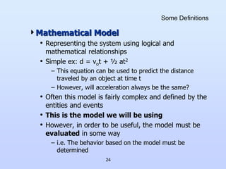
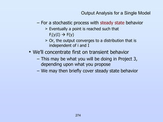
This document provides notes for an introduction to simulation course. It defines key terms like system, entities, events, and different types of models. It explains that simulation is useful for evaluating systems that would be too complex, expensive or dangerous to experiment on directly. The document outlines the goals of the course as understanding simulation concepts, mathematics, programming and implementing simulation projects. It also discusses different approaches to representing time in a simulation, like next-event time advance and fixed-increment time advance.


![52
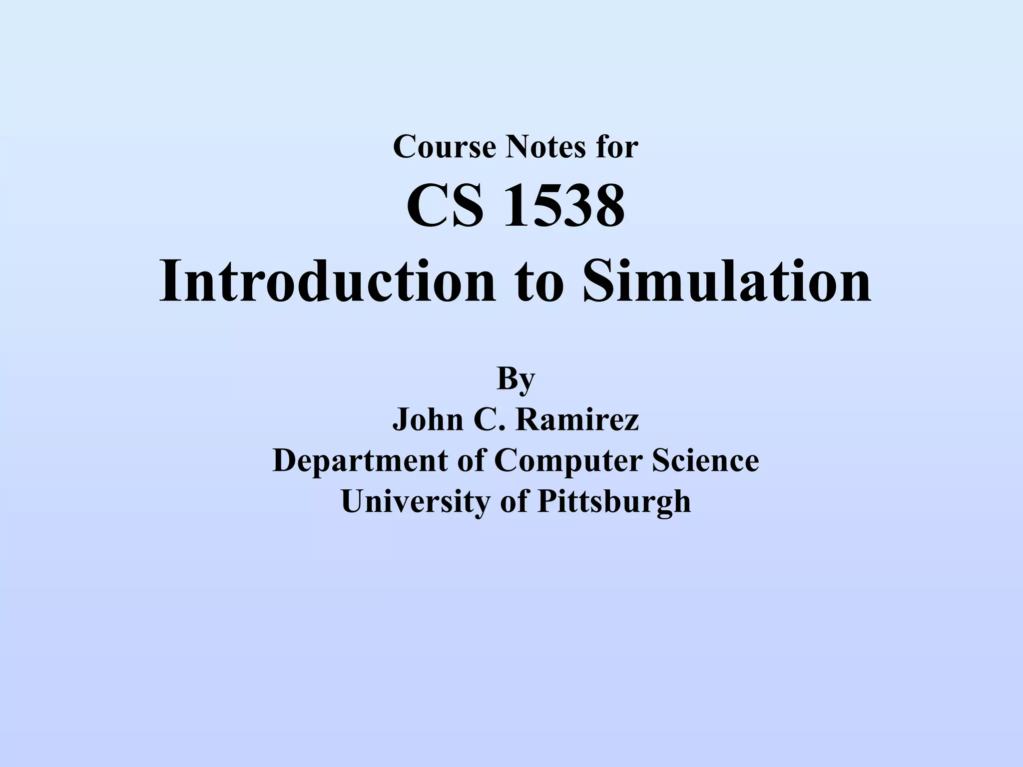
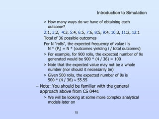
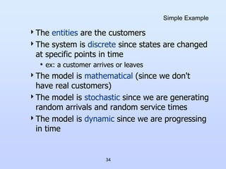
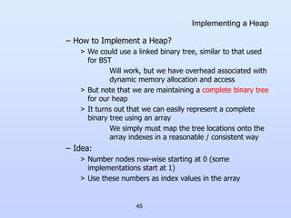
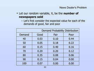
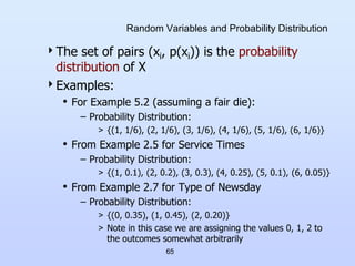
News Dealer's Problem
In fact we do we really need to simulate this
problem at all?
• The data is simple and highly mathematical
• Time is not involved
Let's try to come up with an analytical
solution to this problem
• We have two distributions, the second of which
utilizes the result of the first
• Let's calculate the expected values for random
variables using these distributions
– For a given discrete random variable X, the expected
value,
E(X) = Sum [xi p(xi)] (more soon in Chapter 5)
all i](https://image.slidesharecdn.com/cs1538-230208044806-30a1cd23/85/cs1538-ppt-52-320.jpg)


![69
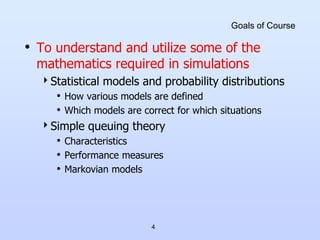
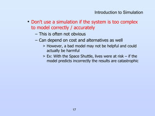
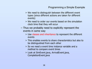
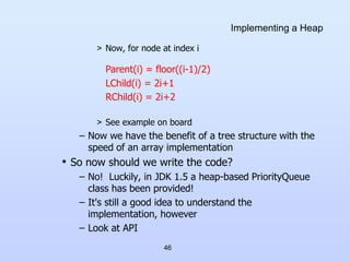
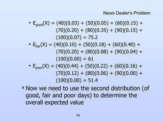
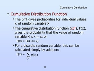
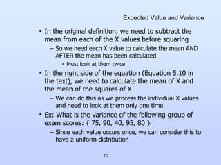
Expected Value and Variance
If each value has the same "probability", we
often add the values together and divide by the
number of values to get the mean (average)
• Ex: Average score on an exam
• Variance
We won't prove the identity, but it is useful
]
])
[
[(
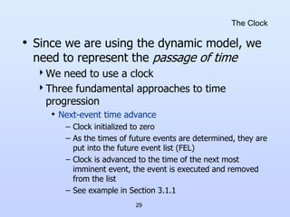
)
( 2
X
E
X
E
X
V
)
10
.
5
(
2
2
)]
(
[
)
( Equation
X
E
X
E
](https://image.slidesharecdn.com/cs1538-230208044806-30a1cd23/85/cs1538-ppt-69-320.jpg)
![71
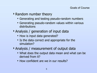
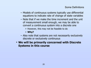
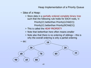
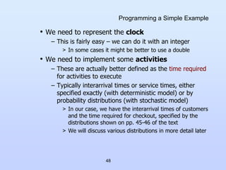
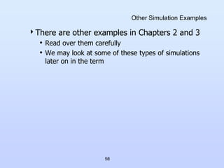
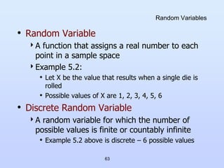
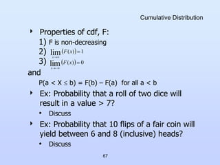
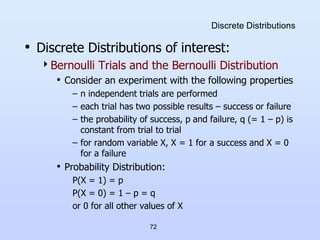
Expected Value and Variance
• V(X) using original definition:
E(X) = (75+90+40+95+80)/5 = 76
V(X) = E[(X – E[X])2] = [(75-76)2 + (90-76)2 + (40-76)2
+ (95-76)2 + (80-76)2]/5
= (1 + 196 + 1296 + 361 + 16)/5 = 374
• V(X) using Equation 5.10
E(X) = (75+90+40+95+80)/5 = 76
E(X2) = (5625+8100+1600+9025+6400)/5 = 6150
V(X) = 6150 – (76)2 = 374
– Note that in this case we can add each number to one
sum and its square to another, so we can calculate
our overall answer with one a single "look" at each
number](https://image.slidesharecdn.com/cs1538-230208044806-30a1cd23/85/cs1538-ppt-71-320.jpg)
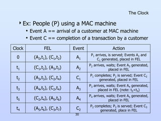
![73
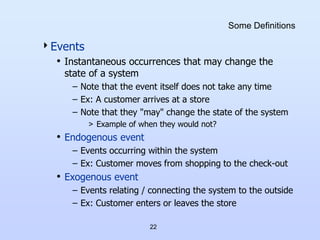
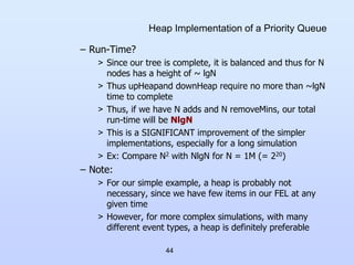
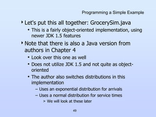
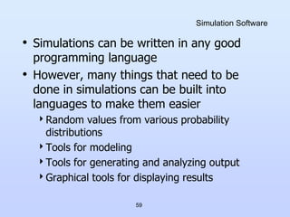
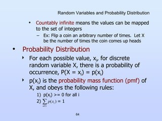
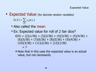
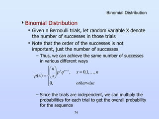
Bernoulli Distribution
• Expected Value
– E(X) = (0)(q) + (1)(p) = p
• Variance
– V(X) = [02q + 12p] – p2 = p(1 – p)
A single Bernoulli trial is not that interesting
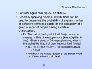
• Typically, multiple trials are performed, from which
we can derive other distributions:
– Binomial Distribution
– Geometric Distribution](https://image.slidesharecdn.com/cs1538-230208044806-30a1cd23/85/cs1538-ppt-73-320.jpg)
![80
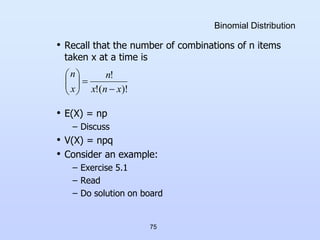
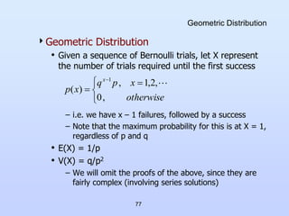
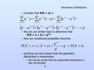
Geometric Distribution
• The conditional probability of an event, A, given that
another event, B, has occurred is defined to be:
• Applying this to the geometric distribution we get
– Clearly, if X > s+t, then X > s (since t cannot be
negative), so we get
)
(
)
(
)
|
(
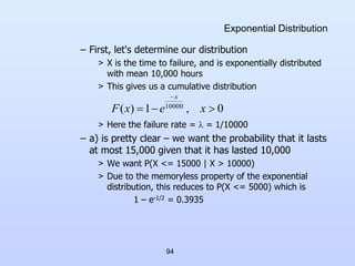
B
P
B
A
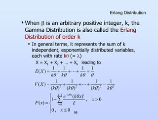
P
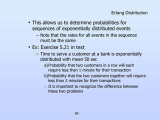
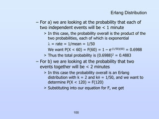
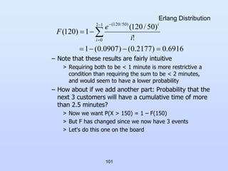
B
A
P
)
(
])
[
]
([
)
|
(
s
X
P
s
X
t
s
X
P
s
X
t
s
X
P
)
(
)
(
)
|
(
s
X
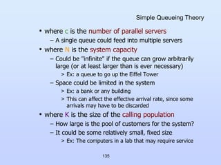
P
t
s
X
P
s
X
t
s
X
P
](https://image.slidesharecdn.com/cs1538-230208044806-30a1cd23/85/cs1538-ppt-80-320.jpg)

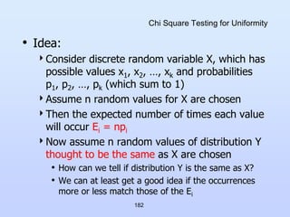
![86
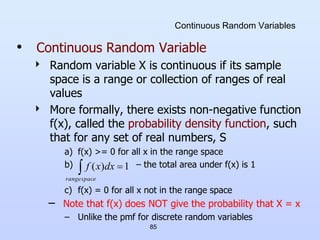
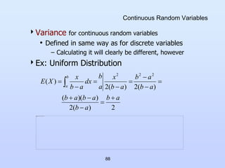
Continuous Random Variables
• The probability that X lies in a given interval [a,b] is
– We see this visually as the "area under the curve"
– Note that for continuous random variables,
P(X = x) = 0 for any x (see from formula above)
– Rather we always look at the probability of x within a
given range (although the range could be very small)
• The cumulative density function (cdf), F(x) is simply
the integral from - to x or
– This gives us the probability up to x
b
a
dx
x
f
b
X
a
P )
(
)
(
x
dt
t
f
x
F )
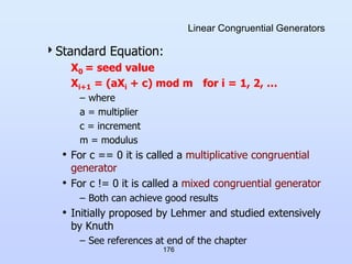
(
)
(](https://image.slidesharecdn.com/cs1538-230208044806-30a1cd23/85/cs1538-ppt-86-320.jpg)
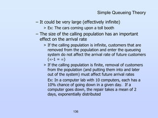
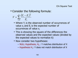
![87
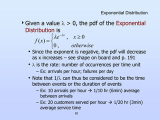
Continuous Random Variables
• Ex: Consider the uniform distribution on the range
[a,b] (see text p. 189)
– Look at plots on board for example range [0,1]
> What about F(x) when x < a or x > b?
Expected Value for a continuous random variable
– Compare to the discrete expected value
otherwise
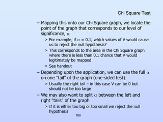
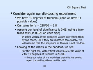
b
x
a
if
a
b
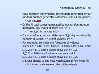
x
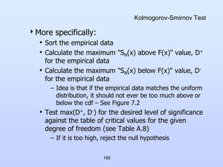
f
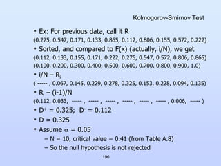
0
1
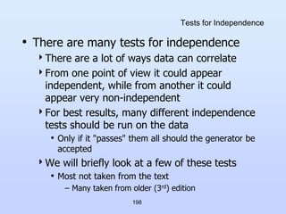
)
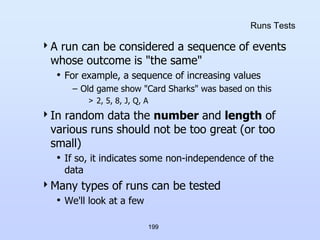
(
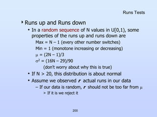
x
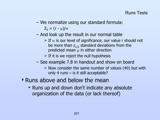
a
x
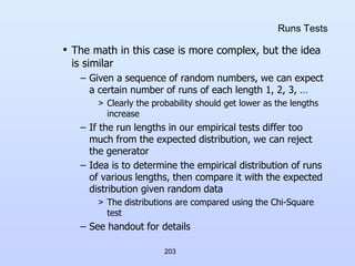
a
b
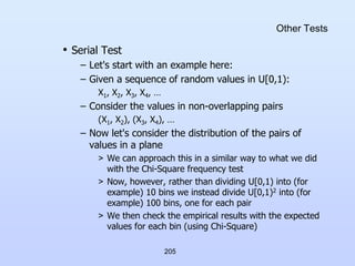
x
a
if
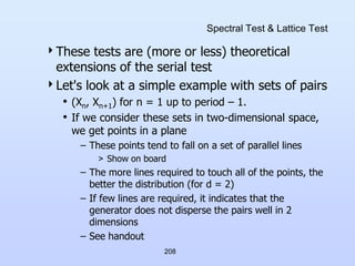
a
b
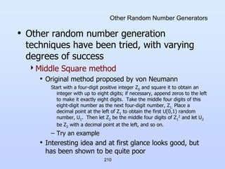
a
x
dy
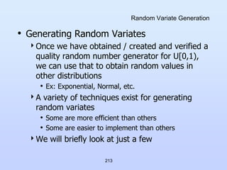
a
b
dy
y
f
x
F
1
)
(
)
(
dx
x
xf
X
E )
(
)
(](https://image.slidesharecdn.com/cs1538-230208044806-30a1cd23/85/cs1538-ppt-87-320.jpg)

(
12
)
(
)
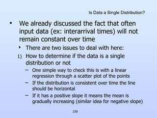
(
3
)
(
12
)
(
4
)
(
4
)
(
)
(
)
(
3
)
(
2
)
)(
(
)
(
3
)
(
2
)
(
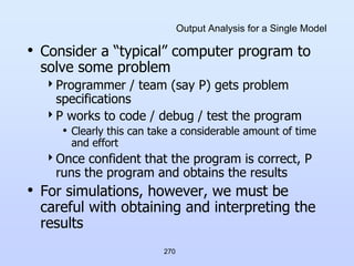
3
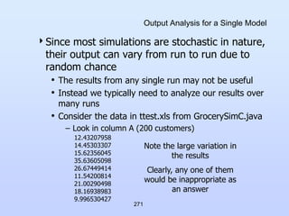
)]
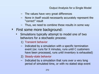
(
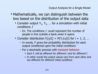
[
)
(
3
)
(
2
3
2
2
3
3
3
2
2
2
2
3
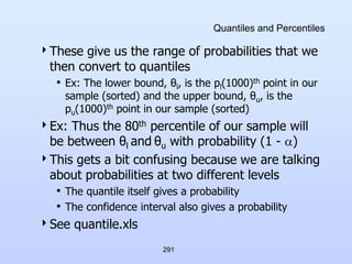
3
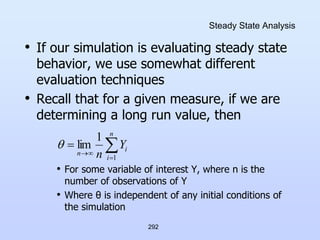
3
2
2
3
3
2
3
3
2
2
2
3
3
2
3
3
2
2
2
3
3
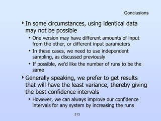
2
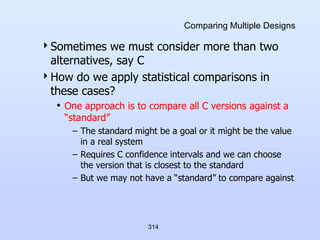
3
a
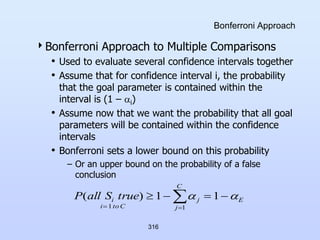
b
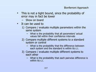
a
b
a
b
a
b
b
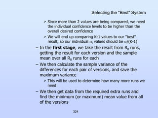
a
ab
a
b
a
b
a
b
a
ab
b
a
ab
b
a
b
a
b
a
b
a
ab
b
a
b
a
b
a
b
a
b
a
b
a
b
a
b
a
b
a
b
a
b
a
b
a
b
a
b
a
b
a
b
a
b
a
b
a
b
a
b
a
b
X
E
a
b
x
a
b
X
V
](https://image.slidesharecdn.com/cs1538-230208044806-30a1cd23/85/cs1538-ppt-89-320.jpg)


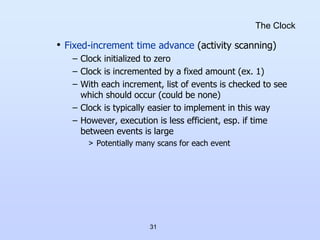
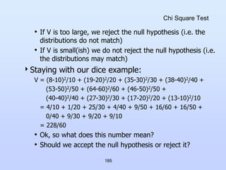
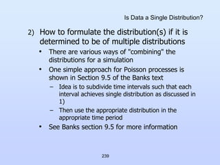
![105
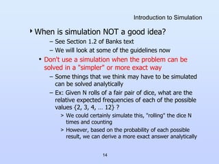
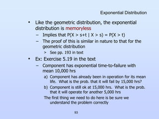
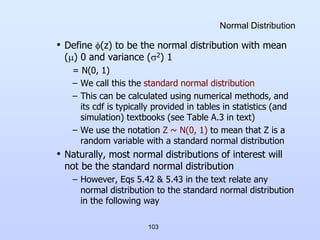
Normal Distribution
– Let Z = (X – 2.4)/0.8
– We want the area under the normal curve with mean
2.4 and standard deviation 0.8 where x > 3.0
This will be 1 – F(3.0)
F(3.0) = [(3.0 – 2.4)/0.8] = (0.75)
– Looking up (0.75) in Table A.3 we find 0.77337
– Recall that we want 1 – F(3.0), which gives us our
final answer of 1 – 0.77337 = 0.2266
• The idea in general is that we are moving from the
mean in units of standard deviations
– The relationship of the mean to standard deviation is
the same for all normal distributions, which is why we
can use the method indicated](https://image.slidesharecdn.com/cs1538-230208044806-30a1cd23/85/cs1538-ppt-105-320.jpg)

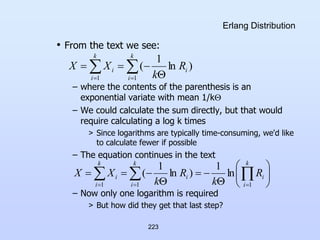
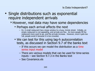
![109
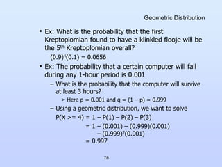
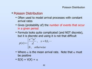
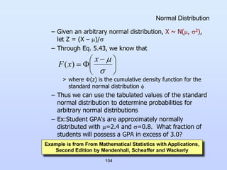
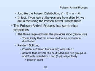
Poisson Arrival Process
1) Arrivals occur one at a time
2) The number of arrivals in a given time period depends
only on the length of that period and not on the starting
point
– i.e. the rate does not change over time
3) The number of arrivals in a given time period does not
affect the number of arrivals in a subsequent period
– i.e. the number of arrivals in given periods are
independent of each other
– Discuss if these are realistic for actual "arrivals"
• We can alter the Poisson distribution to include time
– Only difference is that t is substituted for
otherwise
n
n
t
e
n
t
N
P
n
t
,
0
,
1
,
0
,
!
)
(
]
)
(
[
](https://image.slidesharecdn.com/cs1538-230208044806-30a1cd23/85/cs1538-ppt-109-320.jpg)
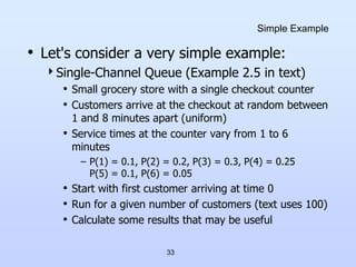
![112
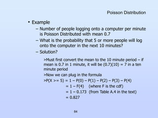
Poisson Arrival Process
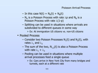
• Ex: Exercise 5.28 in text:
– An average of 30 customers per hour arrive at the
Sticky Donut Ship in accordance with a Poisson
process. What is the probability that more than 5
minutes will elapse before both of the next two
customers walk through the door?
> As usual, the first thing is to identify what it is that we
are trying to solve.
> Discuss (and see Notes)
> Note: We could also model this as Erlang Discuss
– [I added this part] If (on average) 75% of Sticky
Donut Shop's customers get their orders to go, what
is the probability that 3 or more new customers will sit
in the dining room in the next 10 minutes?
> Discuss](https://image.slidesharecdn.com/cs1538-230208044806-30a1cd23/85/cs1538-ppt-112-320.jpg)


![122
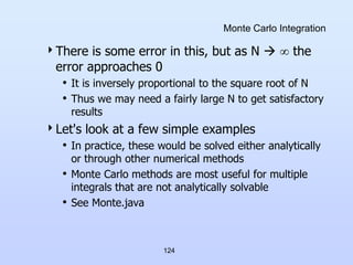
Monte Carlo Integration
Consider function f(x) that is defined and
continuous on the range [a,b]
• The first mean value theorem for integral calculus
states that there exists some number c, with a < c <
b such that:
– The idea is that there is some point within the range
(a,b) that is the "average" height of the curve
– So the area of the rectangle with length (b-a) and
height f(c) is the same as the area under the curve
b
a
b
a
c
f
a
b
dx
x
f
or
c
f
dx
x
f
a
b
)
(
)
(
)
(
)
(
)
(
1](https://image.slidesharecdn.com/cs1538-230208044806-30a1cd23/85/cs1538-ppt-122-320.jpg)
![123
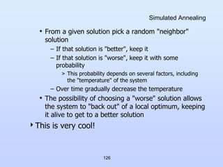
Monte Carlo Integration
So now all we have to do is determine f(c) and
we can evaluate the integral
We can estimate f(c) using Monte Carlo
methods
• Choose N random values x1, … , xN in [a,b]
• Calculate the average (or expected) value, ḟ(x) in
that range:
• Now we can estimate the integral value as
)
(
)
(
1
)
(
1
c
f
x
f
N
x
f
N
i
i
b
a
x
f
a
b
dx
x
f )
(
)
(
)
(](https://image.slidesharecdn.com/cs1538-230208044806-30a1cd23/85/cs1538-ppt-123-320.jpg)


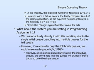
![140
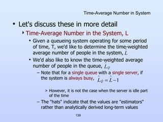
Time-Average Number in System
• We can calculate for an interval [0,T] in a fairly
straightforward manner using a sum:
– Note that each Ti here represents the total time that
the system contained exactly i customers
> These may not be contiguous
– i is shown going to infinity, but in reality most queuing
systems (especially stable queuing systems) will have
all Ti = 0 for i > some value
> In other words, there is some maximum number in the
system that is never exceeded
– See GrocerySimB.java
L
0
1
i
i
T
i
T
L](https://image.slidesharecdn.com/cs1538-230208044806-30a1cd23/85/cs1538-ppt-140-320.jpg)
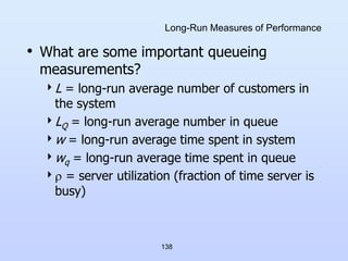
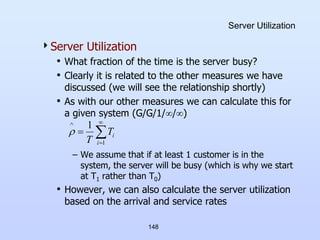
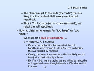
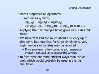
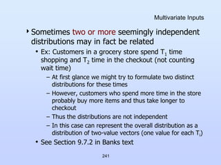
![141
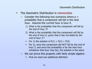
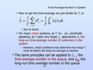
Time-Average Number in System
Let's think of this value in another way:
• Consider the number of customers in the system at
any time, t
– L(t) = number of customers in system at time t
• This value changes as customers enter and leave the
system
• We can graph this with t as the x-axis and L(t) as the
y-axis
• Consider now the area under this plot from [0, T]
– It represents the sum of all of the customers in the
system over all times from [0, T], which can be
determined with an integral
T
dt
t
L
Area
0
)
(](https://image.slidesharecdn.com/cs1538-230208044806-30a1cd23/85/cs1538-ppt-141-320.jpg)
![143
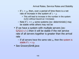
Average Time in System Per Customer
Average Time in System Per Customer, w
• This is also a straightforward calculation during our
simulations
– where N is the number of arrivals in the period [0,T]
– where each Wi is the time customer i spends in the
system during the period [0,T]
• If the system is stable, as N , ŵ w
– w is the long-run average system time
• We can do similar calculations for the queue alone to
get the values ŵQ and wQ
– We can think of these values as the observed delay
and the long-run average delay per customer
N
i
i
W
N
w
1
1](https://image.slidesharecdn.com/cs1538-230208044806-30a1cd23/85/cs1538-ppt-143-320.jpg)

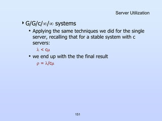


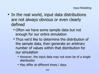
![158
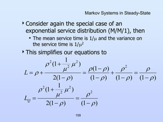
Markov Systems in Steady-State
We can generalize this idea, comparing various
distributions using the coefficient of variation,
cv:
(cv)2 = V(X)/[E(X)]2
– i.e. it is the ratio of the variance to the square of the
expected value
• Distributions that have a larger cv have a larger LQ
for a given server utilization, ρ
– In other words, their LQ values increase more quickly
as ρincreases
– Ex: Consider an exponential service distribution: V(X)
= 1/μ2 and E(X) = 1/μ, so (cv)2 = (1/μ)2/[(1/μ)]2 = 1
> See chart from 4th Edition of text](https://image.slidesharecdn.com/cs1538-230208044806-30a1cd23/85/cs1538-ppt-158-320.jpg)
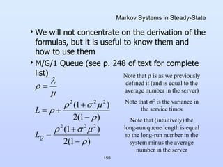
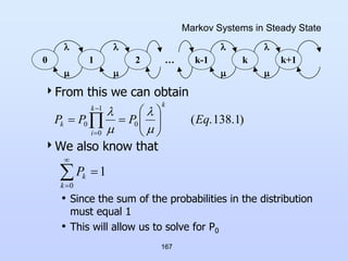
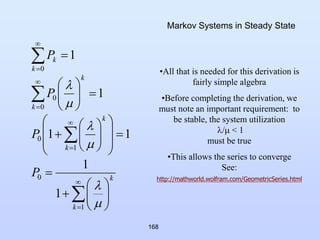
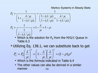
![160
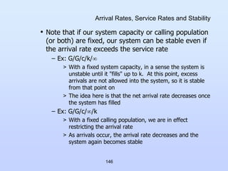
Markov Systems in Steady-State
• The M/M/1 queue gives us a closed form expression
for a measure that the M/G/1 queue does not:
– Pi , the long-run probability that there will be exactly i
customers in the system
– Note: We can use this value to show L for this system
> The last equality is based on the solution to an infinite
geometric series when the base is < 1
> We know ρ < 1 since system must be stable
n
n
P
)
1
(
)
1
1
(
)
1
(
3
3
2
2
0
]
1
[
3
]
1
[
2
]
1
[
1
]
1
[
0
3
2
4
3
3
2
2
3
2
1
0
0
i
i
P
i
L](https://image.slidesharecdn.com/cs1538-230208044806-30a1cd23/85/cs1538-ppt-160-320.jpg)


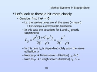
![173
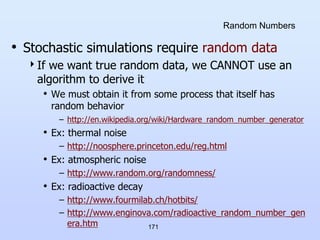
Pseudo-Random Numbers
• Thus, more often than not, simulations rely
on pseudo-random numbers
These numbers are generated deterministically
(i.e. can be reproduced)
However, they have many (most, we hope) of
the properties of true random numbers:
• Numbers are distributed uniformly on [0,1]
– Assuming a generator from [0,1), which is the most
common
• Numbers should show no correlation with each other
– Must appear to be independent
– There are no discernable patterns in the numbers](https://image.slidesharecdn.com/cs1538-230208044806-30a1cd23/85/cs1538-ppt-173-320.jpg)


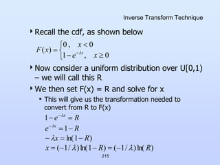
![217
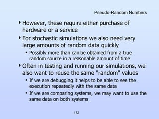
Uniform Distributions on Different Ranges
• Continuous uniform distributions
– Given R U[0,1), we may need to do 2 different
things to get an arbitrary uniform distribution
> Expand (or compress) the range to be larger (or
smaller)
> Shift it to get a different starting point
– The text shows a derivation of the formula, but we
can do it intuitively, based on the two goals above
> To expand the range we need to multiply R by the
length of the range desired
> To get the correct starting point, we need to add (to 0)
the starting point we want
– Consider the desired range [a,b]. Our transformations
yield
X = a + (b – a)R](https://image.slidesharecdn.com/cs1538-230208044806-30a1cd23/85/cs1538-ppt-217-320.jpg)
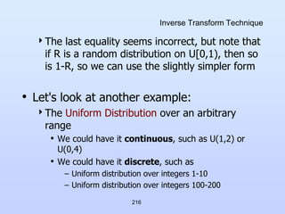
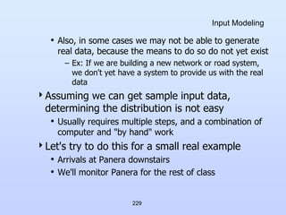
![218
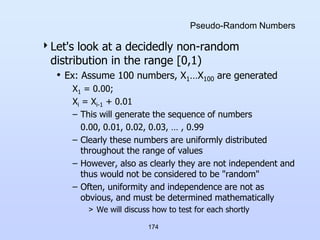
Uniform Distributions on Different Ranges
• Discrete uniform distributions
– The formula in this case is quite similar to that for
the continuous case
– However, care must be paid to the range and any
error due to truncation
– Consider a discrete uniform range [m, n] for integers
m, m+1, … , n-1, n
– If we use
X = m + (n – m)R
> The minimum value is correct, since the minimum
result for X is m (since R can be 0)
> Now we need to be sure of two things:
1) The maximum value is correct
2) The probabilities of all values are the same](https://image.slidesharecdn.com/cs1538-230208044806-30a1cd23/85/cs1538-ppt-218-320.jpg)
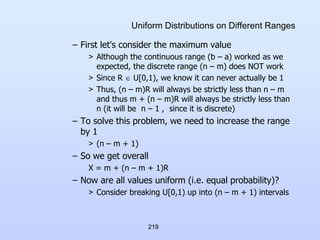
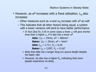
![220
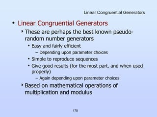
Uniform Distributions on Different Ranges
• Each sub-interval is equal in range and thus has
equal probability
• Given R in each sub-interval, a distinct value in the
range [m,n] will result
– Ex: Assume R is in the second sub-interval above
– We then have
m + (n – m + 1)(1/(n – m + 1)) = m + 1 X <
m + (n – m + 1)(2/(n – m + 1)) = m + 2
– Since X is an integer, and is strictly less than m + 2,
the entire sub-interval maps into m + 1
1
1
,
1
1
2
,
1
1
,
1
1
,
0
m
n
m
n
m
n
m
n
m
n
m
n
m
n
](https://image.slidesharecdn.com/cs1538-230208044806-30a1cd23/85/cs1538-ppt-220-320.jpg)


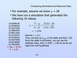
![266
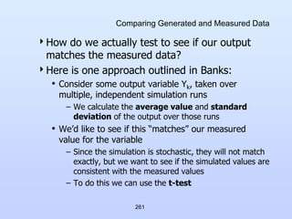
Comparing Generated and Measured Data
– We call (1 – β) the power of the test, and clearly a
high value for (1 – β) [equal to a low value for β] is
desirable
– Unfortunately, for a given value of , the only way to
increase the power of the test (i.e. reduce Type II
error) is to increase the number of points, n
– See ttest.xls for more info
• The existence of Type II errors is why we are
cautious with our Type I error test:
– “We fail to reject the null hypothesis”
– This is also why we looked at the p-values in Chapter
9 when discussing distribution fits
– The better the fit, the higher the p-value and the
lower the chance of Type II errors](https://image.slidesharecdn.com/cs1538-230208044806-30a1cd23/85/cs1538-ppt-266-320.jpg)

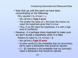
![279
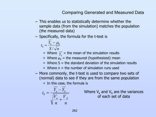
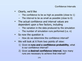
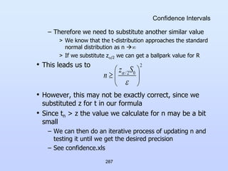
Confidence Intervals
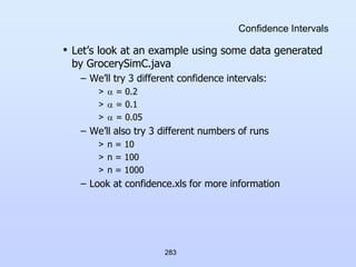
Let’s first look at 1) Given n runs and a
confidence probability, what is our confidence
interval?
• First, we determine the point estimate, Ῡ, for our
distribution
– This is simply
> The mean of the sample points (Equation 11.1)
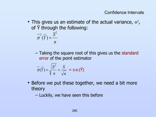
• We next need to determine the sample variance, S2
n
Y
n
j
j
1
1
2
1
2
2
n
Y
n
Y
S
n
j
j
Note: This is the variance formula
E(X2)-[E(X)]2
formula, except that it is dividing by n-1
rather than n, which makes it an
unbiased estimator of the population
variance (see this link)](https://image.slidesharecdn.com/cs1538-230208044806-30a1cd23/85/cs1538-ppt-279-320.jpg)


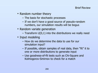
![303
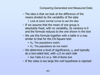
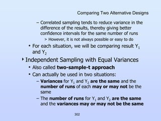
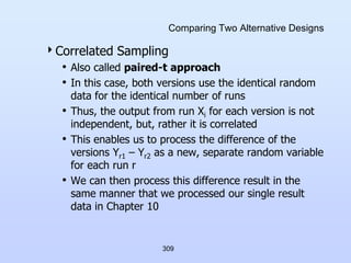
Comparing Two Alternative Designs
First recall what it is that we want to calculate:
• The confidence interval of the difference of the two
results, or
(Ῡ.1 - Ῡ.2) ± t/2,v [s.e.(Ῡ.1 - Ῡ.2)] with prob. (1-)
– To calculate this we need to determine the standard
error for the difference of the two means, and the
degrees of freedom, v
• Consider Ῡ.1 - Ῡ.2 and, more specifically the variance
of Ῡ.1 - Ῡ.2
• Since the runs are independent
Var(Ῡ.1 - Ῡ.2) = Var(Ῡ.1) + Var(Ῡ.2)
= σ1
2/R1 + σ2
2/R2](https://image.slidesharecdn.com/cs1538-230208044806-30a1cd23/85/cs1538-ppt-303-320.jpg)

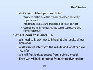
![308
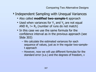
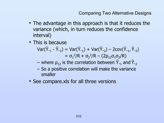
Comparing Two Alternative Designs
• Because the true variances differ, we cannot pool the
sample variances, and must calculate the standard
error using the following equation
• The degrees of freedom is then estimated by
– This technique is actually very old, developed by
Welch in 1938 and discussed [Scheffe, 1970]
2
2
2
1
2
1
2
1
2
1 )
var(
)
var(
)
.(
.
R
S
R
S
Y
Y
Y
Y
e
s
)]
1
/(
)
/
[(
)]
1
/(
)
/
[(
)
/
/
(
2
2
2
2
2
1
2
1
2
1
2
2
2
2
1
2
1
R
R
S
R
R
S
R
S
R
S
v](https://image.slidesharecdn.com/cs1538-230208044806-30a1cd23/85/cs1538-ppt-308-320.jpg)

![322
Comparing Multiple Systems Pairwise
• As mentioned previously, in this case we
have K(K-1)/2 pairs for K different systems
We look for differences pairwise, just as in the
previous technique
However, now we have a lot more pairs to
consider and therefore the individual
probabilities must be a lot higher
• This can present a problem for even a moderate K
• Ex: = 0.1, K = 5
– Each i must be (0.1)/[(5)(4)/2] = 0.01
• Again, this will create either very large intervals or
require a large number of runs](https://image.slidesharecdn.com/cs1538-230208044806-30a1cd23/85/cs1538-ppt-322-320.jpg)