SlideShare a Scribd company logo
1 of 13
OR Unit 8 (III-1Mech) 2014-15
1
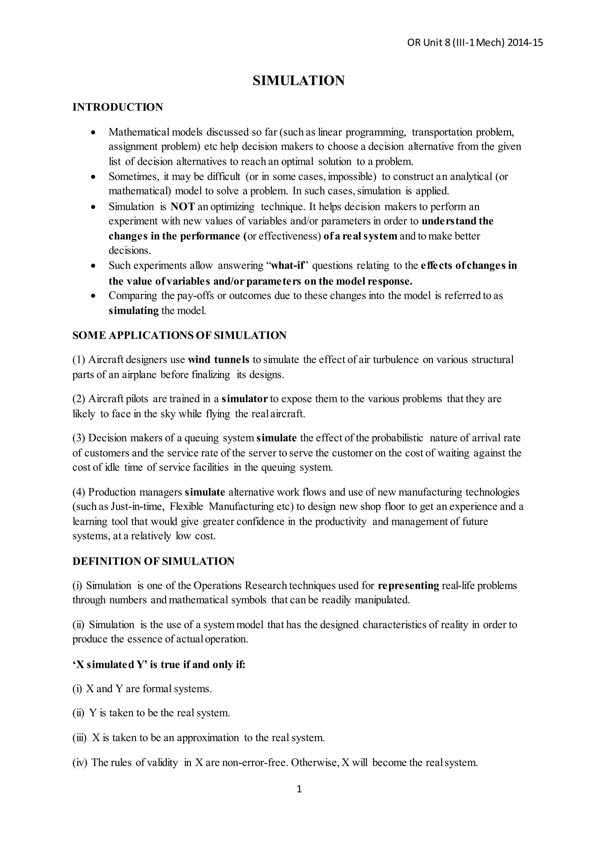
SIMULATION
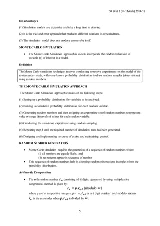
INTRODUCTION
 Mathematical models discussed so far (such as linear programming, transportation problem,
assignment problem) etc help decision makers to choose a decision alternative from the given
list of decision alternatives to reach an optimal solution to a problem.
 Sometimes, it may be difficult (or in some cases,impossible) to construct an analytical (or
mathematical) model to solve a problem. In such cases,simulation is applied.
 Simulation is NOT an optimizing technique. It helps decision makers to perform an
experiment with new values of variables and/or parameters in order to understand the
changes in the performance (or effectiveness) ofa real system and to make better
decisions.
 Such experiments allow answering “what-if” questions relating to the effects ofchanges in
the value ofvariables and/or parameters on the model response.
 Comparing the pay-offs or outcomes due to these changes into the model is referred to as
simulating the model.
SOME APPLICATIONS OF SIMULATION
(1) Aircraft designers use wind tunnels to simulate the effect of air turbulence on various structural
parts of an airplane before finalizing its designs.
(2) Aircraft pilots are trained in a simulator to expose them to the various problems that they are
likely to face in the sky while flying the realaircraft.
(3) Decision makers of a queuing system simulate the effect of the probabilistic nature of arrival rate
of customers and the service rate of the server to serve the customer on the cost of waiting against the
cost of idle time of service facilities in the queuing system.
(4) Production managers simulate alternative work flows and use of new manufacturing technologies
(such as Just-in-time, Flexible Manufacturing etc) to design new shop floor to get an experience and a
learning tool that would give greater confidence in the productivity and management of future
systems, at a relatively low cost.
DEFINITION OF SIMULATION
(i) Simulation is one of the Operations Research techniques used for representing real-life problems
through numbers and mathematical symbols that can be readily manipulated.
(ii) Simulation is the use of a system model that has the designed characteristics of reality in order to
produce the essence of actualoperation.
‘X simulated Y’ is true if and only if:
(i) X and Y are formal systems.
(ii) Y is taken to be the real system.
(iii) X is taken to be an approximation to the real system.
(iv) The rules of validity in X are non-error-free. Otherwise,X will become the realsystem.
OR Unit 8 (III-1Mech) 2014-15
2
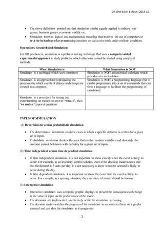
 The above definitions pointed out that simulation can be equally applied to military war
games, business games, economic models etc.
 Simulation involves logical and mathematical modeling that involves the use of computers to
test the behaviour ofa system using iterations or successive trials under realistic conditions.
Operations Research and Simulation
For OR practioners, simulation is a problem solving technique that uses a computer-aided
experimental approach to study problems which otherwise cannot be studied using analytical
methods.
What Simulation is What Simulation is NOT
Simulation is a technique which uses computers Simulation is NOT an analytical technique which
provides an exact solution
Simulation is an approach for reproducing the
processes by which events of chance and change are
created in a computer.
Simulation is NOT a programming language (but it
can be programmed into a set of commands that can
form a language to facilitate the programming of
simulation).
Simulation is a procedure for testing and
experimenting on models to answer “what-if’, then
“so and so” types of questions.
TYPES OF SIMULATION
(1) Deterministic versus probabilistic simulation
 The deterministic simulation involves cases in which a specific outcome is certain for a given
set of inputs.
 Probabilistic simulation deals with cases that involve random variables and obviously the
outcome cannot be known with certainty for a given set of inputs.
(2) Time independent versus time dependent simulation
 In time independent simulation, it is not important to know exactly when the event is likely to
occur. For example, in an inventory control solution, even if the decision maker knows that
that the demand is 3 units per day, it is not necessary to know when the demand is likely to
occur during the day.
 In time dependent simulation, it is important to know the exact time the event is likely to
occur. For example, in a queuing situation, the exact time of arrival should be known.
(3) Interactive simulation
 Interactive simulation uses computer graphic displays to present the consequences of change
in the value of input on the performance of the model.
 The decisions are implemented interactively while the simulation is running.
 The decision maker watches the progress of the simulation in an animated form on a graphic
terminal and can alter the simulation as it progresses.
OR Unit 8 (III-1Mech) 2014-15
3
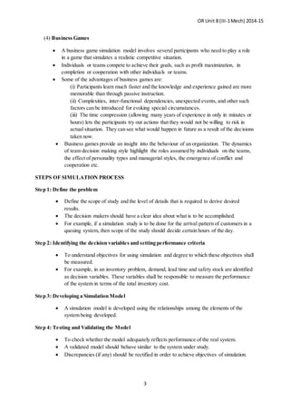
(4) Business Games
 A business game simulation model involves several participants who need to play a role
in a game that simulates a realistic competitive situation.
 Individuals or teams compete to achieve their goals, such as profit maximization, in
completion or cooperation with other individuals or teams.
 Some of the advantages of business games are:
(i) Participants learn much faster and the knowledge and experience gained are more
memorable than through passive instruction.
(ii) Complexities, inter-functional dependencies, unexpected events, and other such
factors can be introduced for evoking special circumstances.
(iii) The time compression (allowing many years of experience in only in minutes or
hours) lets the participants try out actions that they would not be willing to risk in
actual situation. They can see what would happen in future as a result of the decisions
taken now.
 Business games provide an insight into the behaviour of an organization. The dynamics
of team decision making style highlight the roles assumed by individuals on the teams,
the effect of personality types and managerial styles, the emergence of conflict and
cooperation etc.
STEPS OF SIMULATION PROCESS
Step 1: Define the problem
 Define the scope of study and the level of details that is required to derive desired
results.
 The decision makers should have a clear idea about what is to be accomplished.
 For example, if a simulation study is to be done for the arrival pattern of customers in a
queuing system, then scope of the study should decide certain hours of the day.
Step 2: Identifying the decision variables and setting performance criteria
 To understand objectives for using simulation and degree to which these objectives shall
be measured.
 For example, in an inventory problem, demand, lead time and safety stock are identified
as decision variables. These variables shall be responsible to measure the performance
of the system in terms of the total inventory cost.
Step 3: Developing a Simulation Model
 A simulation model is developed using the relationships among the elements of the
system being developed.
Step 4: Testing and Validating the Model
 To check whether the model adequately reflects performance of the real system.
 A validated model should behave similar to the system under study.
 Discrepancies (if any) should be rectified in order to achieve objectives of simulation.
OR Unit 8 (III-1Mech) 2014-15
4
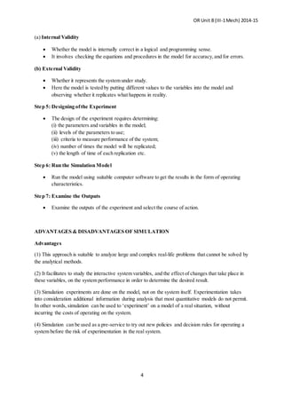
(a) Internal Validity
 Whether the model is internally correct in a logical and programming sense.
 It involves checking the equations and procedures in the model for accuracy,and for errors.
(b) External Validity
 Whether it represents the system under study.
 Here the model is tested by putting different values to the variables into the model and
observing whether it replicates what happens in reality.
Step 5: Designing ofthe Experiment
 The design of the experiment requires determining:
(i) the parameters and variables in the model;
(ii) levels of the parameters to use;
(iii) criteria to measure performance of the system;
(iv) number of times the model will be replicated;
(v) the length of time of each replication etc.
Step 6: Run the Simulation Model
 Run the model using suitable computer software to get the results in the form of operating
characteristics.
Step 7: Examine the Outputs
 Examine the outputs of the experiment and select the course of action.
ADVANTAGES & DISADVANTAGES OF SIMULATION
Advantages
(1) This approach is suitable to analyze large and complex real-life problems that cannot be solved by
the analytical methods.
(2) It facilitates to study the interactive system variables, and the effect of changes that take place in
these variables, on the system performance in order to determine the desired result.
(3) Simulation experiments are done on the model, not on the system itself. Experimentation takes
into consideration additional information during analysis that most quantitative models do not permit.
In other words, simulation can be used to ‘experiment’ on a model of a real situation, without
incurring the costs of operating on the system.
(4) Simulation can be used as a pre-service to try out new policies and decision rules for operating a
system before the risk of experimentation in the real system.
OR Unit 8 (III-1Mech) 2014-15
5
Disadvantages
(1) Simulation models are expensive and take a long time to develop.
(2) It is the trial and error approach that produces different solutions in repeated runs.
(3) The simulation model does not produce answers by itself.
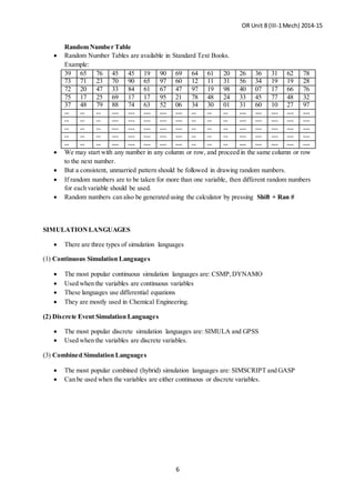
MONTE CARLO SIMULATION
 The Monte Carlo Simulation approach is used to incorporate the random behaviour of
variable (s) of interest in a model.
Definition
The Monte Carlo simulation technique involves conducting repetitive experiments on the model of the
system under study, with some known probability distribution to draw random samples (observations)
using random numbers.
THE MONTE CARLO SIMULATION APPROACH
The Monte Carlo Simulation approach consists of the following steps:
(1) Setting up a probability distribution for variables to be analyzed.
(2) Building a cumulative probability distribution for each random variable,
(3) Generating random numbers and then assigning an appropriate set of random numbers to represent
value or range (interval) of values for each random variable.
(4) Conducting the simulation experiment using random sampling.
(5) Repeating step 4 until the required number of simulation runs has been generated.
(6) Designing and implementing a course of action and maintaining control.
RANDOM NUMBER GENERATION
 Monte Carlo simulation requires the generation of a sequence of random numbers where
(i) all numbers are equally likely, and
(ii) no patterns appear in sequence of number
 This sequence of random numbers help in choosing random observations (samples) from the
probability distributions.
Arithmetic Computation
 The n th random number rn, consisting of k digits, generated by using multiplicative
congruential method is given by:
rn = p.rn-1 (modulo m)
where p and m are positive integers, p < m, rn-1 is a k digit number and modulo means
rn is the remainder when p.rn-1 is divided by m.
OR Unit 8 (III-1Mech) 2014-15
6
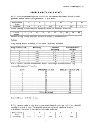
Random Number Table
 Random Number Tables are available in Standard Text Books.
Example:
39 65 76 45 45 19 90 69 64 61 20 26 36 31 62 78
73 71 23 70 90 65 97 60 12 11 31 56 34 19 19 28
72 20 47 33 84 61 67 47 97 19 98 40 07 17 66 76
75 17 25 69 17 17 95 21 78 48 24 33 45 77 48 32
37 48 79 88 74 63 52 06 34 30 01 31 60 10 27 97
-- -- -- --- --- --- --- --- -- -- -- --- --- --- --- ---
-- -- -- --- --- --- --- --- -- -- -- --- --- --- --- ---
-- -- -- --- --- --- --- --- -- -- -- --- --- --- --- ---
-- -- -- --- --- --- --- --- -- -- -- --- --- --- --- ---
-- -- -- --- --- --- --- --- -- -- -- --- --- --- --- ---
 We may start with any number in any column or row, and proceed in the same column or row
to the next number.
 But a consistent, unmarried pattern should be followed in drawing random numbers.
 If random numbers are to be taken for more than one variable, then different random numbers
for each variable should be used.
 Random numbers can also be generated using the calculator by pressing Shift + Ran #
SIMULATIONLANGUAGES
 There are three types of simulation languages
(1) Continuous Simulation Languages
 The most popular continuous simulation languages are: CSMP,DYNAMO
 Used when the variables are continuous variables
 These languages use differential equations
 They are mostly used in Chemical Engineering.
(2) Discrete Event Simulation Languages
 The most popular discrete simulation languages are: SIMULA and GPSS
 Used when the variables are discrete variables.
(3) Combined Simulation Languages
 The most popular combined (hybrid) simulation languages are: SIMSCRIPT and GASP
 Can be used when the variables are either continuous or discrete variables.
OR Unit 8 (III-1Mech) 2014-15
7
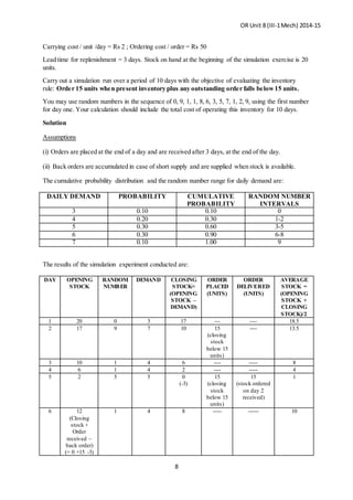
PROBLEMS ON SIMULATION
Q (1) A bakery keeps stock of a popular brand of cake. Previous experience shows the daily demand
pattern for the item with associated probabilities, as given below:
Daily demand
(Units)
0 10 20 30 40 50
Probability 0.01 0.20 0.15 0.50 0.12 0.02
Use the following sequence of random numbers to simulate the demand for next 10 days.
Random
number
25 39 65 76 12 05 73 89 19 49
Estimate the daily average demand for the cakes on the basis of the simulated data.
Solution
Using the daily demand distribution, we first obtain a probability distribution.
Daily demand (Units) Probability Cumulative
Probability
Random Number
Intervals
0 0.01 0.01 00
10 0.20 0.21 01-20
20 0.15 0.36 21-35
30 0.50 0.86 36-85
40 0.12 0.98 86-97
50 0.12 1.00 98-99
Next to conduct a simulation experiment for demand, take a sample of random numbers. They
represent the sequence of 10 samples.
DAYS RANDOM NUMBER SIMULATED DEMAND
1 25 20
2 39 30
3 65 30
4 76 30
5 12 10
6 05 10
7 73 30
8 89 40
9 19 10
10 49 30
TOTAL DEMAND 240
Expected demand = (240/10) = 24 units.
Q (2) A company trading in motor vehicle spare parts wishes to determine the levels of stock it should
carry for the items in its range. The demand is not certain and there is a lead time for stock
replenishment. For an item A, the following information is obtained.
Daily demand
(Units)
3 4 5 6 7
Probability 0.10 0.20 0.30 0.30 0.10
OR Unit 8 (III-1Mech) 2014-15
8
Carrying cost / unit /day = Rs 2 ; Ordering cost / order = Rs 50
Lead time for replenishment = 3 days. Stock on hand at the beginning of the simulation exercise is 20
units.
Carry out a simulation run over a period of 10 days with the objective of evaluating the inventory
rule: Order 15 units when present inventory plus any outstanding order falls below15 units.
You may use random numbers in the sequence of 0, 9, 1, 1, 8, 6, 3, 5, 7, 1, 2, 9, using the first number
for day one. Your calculation should include the total cost of operating this inventory for 10 days.
Solution
Assumptions
(i) Orders are placed at the end of a day and are received after 3 days, at the end of the day.
(ii) Back orders are accumulated in case of short supply and are supplied when stock is available.
The cumulative probability distribution and the random number range for daily demand are:
DAILY DEMAND PROBABILITY CUMULATIVE
PROBABILITY
RANDOM NUMBER
INTERVALS
3 0.10 0.10 0
4 0.20 0.30 1-2
5 0.30 0.60 3-5
6 0.30 0.90 6-8
7 0.10 1.00 9
The results of the simulation experiment conducted are:
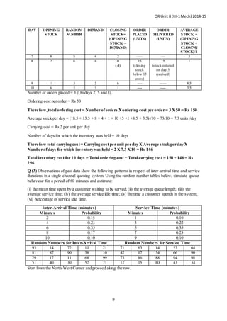
DAY OPENING
STOCK
RANDOM
NUMBER
DEMAND CLOSING
STOCK=
(OPENING
STOCK –
DEMAND)
ORDER
PLACED
(UNITS)
ORDER
DELIVERED
(UNITS)
AVERAGE
STOCK =
(OPENING
STOCK +
CLOSING
STOCK)/2
1 20 0 3 17 --- ---- 18.5
2 17 9 7 10 15
(closing
stock
below 15
units)
---- 13.5
3 10 1 4 6 ---- ----- 8
4 6 1 4 2 ---- ----- 4
5 2 5 5 0
(-3)
15
(closing
stock
below 15
units)
15
(stock ordered
on day 2
received)
1
6 12
(Closing
stock +
Order
received –
back order)
(= 0 +15 -3)
1 4 8 ----- ------ 10
OR Unit 8 (III-1Mech) 2014-15
9
DAY OPENING
STOCK
RANDOM
NUMBER
DEMAND CLOSING
STOCK=
(OPENING
STOCK –
DEMAND)
ORDER
PLACED
(UNITS)
ORDER
DELIVERED
(UNITS)
AVERAGE
STOCK =
(OPENING
STOCK +
CLOSING
STOCK)/2
7 8 8 6 2 ----- ---- 5
8 2 6 6 0
(-4)
15
(closing
stock
below 15
units)
15
(stock ordered
on day 5
received)
1
9 11 3 5 6 ---- ------ 8.5
10 6 5 5 1 ---- ----- 3.5
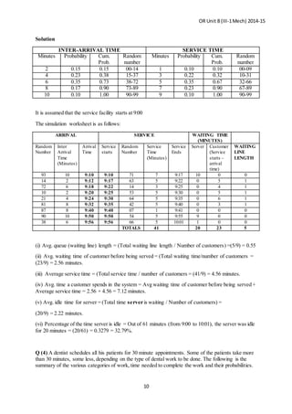
Number of orders placed = 3 (On days 2, 5 and 8).
Ordering cost per order = Rs 50
Therefore,total ordering cost = Number oforders Xordering cost per order = 3 X50 = Rs 150
Average stock per day = (18.5 + 13.5 + 8 + 4 + 1 + 10 +5 +1 +8.5 + 3.5) /10 = 73/10 = 7.3 units /day
Carrying cost = Rs 2 per unit per day
Number of days for which the inventory was held = 10 days
Therefore total carrying cost= Carrying cost per unit per day X Average stock per day X
Number of days for which inventory was held = 2 X7.3 X10 = Rs 146
Total inventory cost for 10 days = Total ordering cost + Total carrying cost = 150 + 146 = Rs
296.
Q (3) Observations of past data show the following patterns in respect of inter-arrival time and service
durations in a single-channel queuing system. Using the random number tables below, simulate queue
behaviour for a period of 60 minutes and estimate:
(i) the mean time spent by a customer waiting to be served; (ii) the average queue length; (iii) the
average service time; (iv) the average service idle time; (v) the time a customer spends in the system;
(vi) percentage of service idle time.
Inter-Arrival Time (minutes) Service Time (minutes)
Minutes Probability Minutes Probability
2 0.15 1 0.10
4 0.23 3 0.22
6 0.35 5 0.35
8 0.17 7 0.23
10 0.10 9 0.10
Random Numbers for Inter-Arrival Time Random Numbers for Service Time
93 14 72 10 21 71 63 14 53 64
81 87 90 38 10 42 07 54 66 90
29 17 11 68 99 73 86 88 94 98
51 40 30 52 71 12 15 80 43 34
Start from the North-West Corner and proceed along the row.
OR Unit 8 (III-1Mech) 2014-15
10
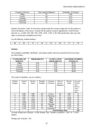
Solution
INTER-ARRIVAL TIME SERVICE TIME
Minutes Probability Cum.
Prob.
Random
number
Minutes Probability Cum.
Prob.
Random
number
2 0.15 0.15 00-14 1 0.10 0.10 00-09
4 0.23 0.38 15-37 3 0.22 0.32 10-31
6 0.35 0.73 38-72 5 0.35 0.67 32-66
8 0.17 0.90 73-89 7 0.23 0.90 67-89
10 0.10 1.00 90-99 9 0.10 1.00 90-99
It is assumed that the service facility starts at 9:00
The simulation worksheet is as follows:
ARRIVAL SERVICE WAITING TIME
(MINUTES)
Random
Number
Inter
Arrival
Time
(Minutes)
Arrival
Time
Service
starts
Random
Number
Service
Time
(Minutes)
Service
Ends
Server Customer
(Service
starts –
arrival
time)
WAITING
LINE
LENGTH
93 10 9:10 9:10 71 7 9:17 10 0 0
14 2 9:12 9:17 63 5 9:22 0 5 1
72 6 9:18 9:22 14 3 9:25 0 4 1
10 2 9:20 9:25 53 5 9:30 0 5 1
21 4 9:24 9:30 64 5 9:35 0 6 1
81 8 9:32 9:35 42 5 9:40 0 3 1
87 8 9:40 9:40 07 1 9:41 0 0 0
90 10 9:50 9:50 54 5 9:55 9 0 0
38 6 9:56 9:56 66 5 10:01 1 0 0
TOTALS 41 20 23 5
(i) Avg. queue (waiting line) length = (Total waiting line length / Number of customers) =(5/9) = 0.55
(ii) Avg. waiting time of customer before being served = (Total waiting time/number of customers =
(23/9) = 2.56 minutes.
(iii) Average service time = (Total service time / number of customers = (41/9) = 4.56 minutes.
(iv) Avg. time a customer spends in the system = Avg waiting time of customer before being served +
Average service time = 2.56 + 4.56 = 7.12 minutes.
(v) Avg. idle time for server = (Total time server is waiting / Number of customers) =
(20/9) = 2.22 minutes.
(vi) Percentage of the time server is idle = Out of 61 minutes (from 9:00 to 10:01), the server was idle
for 20 minutes = (20/61) = 0.3279 = 32.79%.
Q (4) A dentist schedules all his patients for 30 minute appointments. Some of the patients take more
than 30 minutes, some less, depending on the type of dental work to be done. The following is the
summary of the various categories of work, time needed to complete the work and their probabilities.
OR Unit 8 (III-1Mech) 2014-15
11
Category of Service Time required (Minutes) Probability of Category
Filling 45 0.40
Crown 60 0.15
Cleaning 15 0.15
Extraction 45 0.10
Check-up 15 0.20
Simulate the dentist’s clinic for four hours and determine the average waiting time for the patients as
well as the idleness of the doctor. Assume that the patients are given appointments at half-an-hour
intervals (i.e., at 8:00, 8:30, 9:00, 9:30, 10:00, 10:30, 11:00, 11:30 AM) and that they show up at the
clinic at exactly their scheduled arrival time.
Use the following random numbers:
40 82 11 34 25 66 17 79
Solution
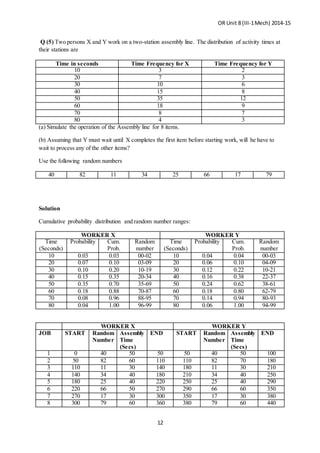
The cumulative probability distribution and random number intervals associated with service times
are shown below:
CATEGORY OF
SERVICE
PROBABILITY CUMULATIVE
PROBABILITY
RANDOM NUMBER
INTERVAL
Filling 0.40 0.40 00-39
Crown 0.15 0.55 40-54
Cleaning 0.15 0.70 55-69
Extraction 0.10 0.80 70-79
Checkup 0.20 1.00 80-99
The results of simulation run are as follows:
Patient
Number
Arrival
Time
Service
Starts
Random
Number
Category
of Service
Time of
Service
(Minutes)
Service
Ends
Customer
Waiting
Time
(Service
starts –
arrival
time)
1 8:00 8:00 40 Crown 60 9:00 0
2 8:30 9:00 82 Check up 15 9:15 30
3 9:00 9:15 11 Filling 45 10:00 15
4 9:30 10:00 34 Filling 45 10:45 30
5 10:00 10:45 25 Filling 45 11:30 45
6 10:30 11:30 66 Cleaning 15 11:45 60
7 11:00 11:45 17 Filling 45 12:30 45
8 11:30 12:30 79 Extraction 45 1:15 60
Total Waiting Time 285
Average waiting time of patient = (Total Waiting Time / Number of patients) = (285 / 8) = 35.625
minutes.
Waiting time of dentist = Nil
OR Unit 8 (III-1Mech) 2014-15
12
Q (5) Two persons X and Y work on a two-station assembly line. The distribution of activity times at
their stations are
Time in seconds Time Frequency for X Time Frequency for Y
10 3 2
20 7 3
30 10 6
40 15 8
50 35 12
60 18 9
70 8 7
80 4 3
(a) Simulate the operation of the Assembly line for 8 items.
(b) Assuming that Y must wait until X completes the first item before starting work, will he have to
wait to process any of the other items?
Use the following random numbers
40 82 11 34 25 66 17 79
Solution
Cumulative probability distribution and random number ranges:
WORKER X WORKER Y
Time
(Seconds)
Probability Cum.
Prob.
Random
number
Time
(Seconds)
Probability Cum.
Prob.
Random
number
10 0.03 0.03 00-02 10 0.04 0.04 00-03
20 0.07 0.10 03-09 20 0.06 0.10 04-09
30 0.10 0.20 10-19 30 0.12 0.22 10-21
40 0.15 0.35 20-34 40 0.16 0.38 22-37
50 0.35 0.70 35-69 50 0.24 0.62 38-61
60 0.18 0.88 70-87 60 0.18 0.80 62-79
70 0.08 0.96 88-95 70 0.14 0.94 80-93
80 0.04 1.00 96-99 80 0.06 1.00 94-99
WORKER X WORKER Y
JOB START Random
Number
Assembly
Time
(Secs)
END START Random
Number
Assembly
Time
(Secs)
END
1 0 40 50 50 50 40 50 100
2 50 82 60 110 110 82 70 180
3 110 11 30 140 180 11 30 210
4 140 34 40 180 210 34 40 250
5 180 25 40 220 250 25 40 290
6 220 66 50 270 290 66 60 350
7 270 17 30 300 350 17 30 380
8 300 79 60 360 380 79 60 440
OR Unit 8 (III-1Mech) 2014-15
13

More Related Content

What's hot

Operation research ppt chapter one
Operation research ppt   chapter oneOperation research ppt   chapter one
Operation research ppt chapter onemitku assefa
 
Operations research - an overview
Operations research -  an overviewOperations research -  an overview
Operations research - an overviewJoseph Konnully
 
Applications of simulation in Business with Example
Applications of simulation in Business with ExampleApplications of simulation in Business with Example
Applications of simulation in Business with ExamplePratima Ray
 
Sequencing problems in Operations Research
Sequencing problems in Operations ResearchSequencing problems in Operations Research
Sequencing problems in Operations ResearchAbu Bashar
 
Assembly Line Balancing -Example
Assembly Line Balancing -ExampleAssembly Line Balancing -Example
Assembly Line Balancing -ExampleJoseph Konnully
 
Queueing Theory and its BusinessS Applications
Queueing Theory and its BusinessS ApplicationsQueueing Theory and its BusinessS Applications
Queueing Theory and its BusinessS ApplicationsBiswajit Bhattacharjee
 
Queuing theory
Queuing theoryQueuing theory
Queuing theoryAmit Sinha
 
Introduction to Operations Research
Introduction to Operations ResearchIntroduction to Operations Research
Introduction to Operations ResearchSundar B N
 
Replacement theory
Replacement theoryReplacement theory
Replacement theoryVILAS ADOLE
 
Transportation and Assignment
Transportation and AssignmentTransportation and Assignment
Transportation and AssignmentLokesh Payasi
 
Introduction to simulation modeling
Introduction to simulation modelingIntroduction to simulation modeling
Introduction to simulation modelingbhupendra kumar
 
MODI Method (Operations Research)
MODI Method (Operations Research) MODI Method (Operations Research)
MODI Method (Operations Research) Nilraj Vasandia
 
types of facility layout algorithm
types of facility layout algorithmtypes of facility layout algorithm
types of facility layout algorithmAsIf Fisa
 
Operation's research models
Operation's research modelsOperation's research models
Operation's research modelsAbhinav Kp
 

What's hot (20)

Operation research ppt chapter one
Operation research ppt   chapter oneOperation research ppt   chapter one
Operation research ppt chapter one
 
Operations research - an overview
Operations research -  an overviewOperations research -  an overview
Operations research - an overview
 
Applications of simulation in Business with Example
Applications of simulation in Business with ExampleApplications of simulation in Business with Example
Applications of simulation in Business with Example
 
Sequencing problems in Operations Research
Sequencing problems in Operations ResearchSequencing problems in Operations Research
Sequencing problems in Operations Research
 
Queueing theory
Queueing theoryQueueing theory
Queueing theory
 
Assembly Line Balancing -Example
Assembly Line Balancing -ExampleAssembly Line Balancing -Example
Assembly Line Balancing -Example
 
Queueing Theory and its BusinessS Applications
Queueing Theory and its BusinessS ApplicationsQueueing Theory and its BusinessS Applications
Queueing Theory and its BusinessS Applications
 
Game theory
Game theoryGame theory
Game theory
 
Queuing theory
Queuing theoryQueuing theory
Queuing theory
 
Introduction to Operations Research
Introduction to Operations ResearchIntroduction to Operations Research
Introduction to Operations Research
 
Replacement theory
Replacement theoryReplacement theory
Replacement theory
 
Assignment problems
Assignment problemsAssignment problems
Assignment problems
 
Transportation and Assignment
Transportation and AssignmentTransportation and Assignment
Transportation and Assignment
 
Assignment Problem
Assignment ProblemAssignment Problem
Assignment Problem
 
Introduction to simulation modeling
Introduction to simulation modelingIntroduction to simulation modeling
Introduction to simulation modeling
 
Goal programming
Goal programmingGoal programming
Goal programming
 
Unit i-2-dt
Unit i-2-dtUnit i-2-dt
Unit i-2-dt
 
MODI Method (Operations Research)
MODI Method (Operations Research) MODI Method (Operations Research)
MODI Method (Operations Research)
 
types of facility layout algorithm
types of facility layout algorithmtypes of facility layout algorithm
types of facility layout algorithm
 
Operation's research models
Operation's research modelsOperation's research models
Operation's research models
 

Viewers also liked

Chp. 2 simulation examples
Chp. 2 simulation examplesChp. 2 simulation examples
Chp. 2 simulation examplesPravesh Negi
 
Simulation Techniques
Simulation TechniquesSimulation Techniques
Simulation Techniquesmailrenuka
 
QUEUING THEORY
QUEUING THEORYQUEUING THEORY
QUEUING THEORYavtarsingh
 
System simulation & modeling notes[sjbit]
System simulation & modeling notes[sjbit]System simulation & modeling notes[sjbit]
System simulation & modeling notes[sjbit]qwerty626
 
Classbfs121001503719748
Classbfs121001503719748Classbfs121001503719748
Classbfs121001503719748Raju Panthadi
 
A comparative study of initial basic feasible solution methods
A comparative study of initial basic feasible solution methodsA comparative study of initial basic feasible solution methods
A comparative study of initial basic feasible solution methodsAlexander Decker
 
Transportation lecture
Transportation lectureTransportation lecture
Transportation lectureMoudud Hasan
 
BC 504-Operation Research
BC 504-Operation ResearchBC 504-Operation Research
BC 504-Operation ResearchPCTE
 
Assignment oprations research luv
Assignment oprations research luvAssignment oprations research luv
Assignment oprations research luvAshok Sharma
 
Queuing theory and simulation (MSOR)
Queuing theory and simulation (MSOR)Queuing theory and simulation (MSOR)
Queuing theory and simulation (MSOR)snket
 
heizer jay operations management Ch08pp
heizer jay operations management Ch08ppheizer jay operations management Ch08pp
heizer jay operations management Ch08ppTaliya Hemanth
 

Viewers also liked (20)

Chp. 2 simulation examples
Chp. 2 simulation examplesChp. 2 simulation examples
Chp. 2 simulation examples
 
OR 14 15-unit_2
OR 14 15-unit_2OR 14 15-unit_2
OR 14 15-unit_2
 
OR 14 15-unit_4
OR 14 15-unit_4OR 14 15-unit_4
OR 14 15-unit_4
 
Unit 7 dynamic programming
Unit 7   dynamic programmingUnit 7   dynamic programming
Unit 7 dynamic programming
 
OR 14 15-unit_1
OR 14 15-unit_1OR 14 15-unit_1
OR 14 15-unit_1
 
OR Unit 5 queuing theory
OR Unit 5 queuing theoryOR Unit 5 queuing theory
OR Unit 5 queuing theory
 
Simulation Techniques
Simulation TechniquesSimulation Techniques
Simulation Techniques
 
QUEUING THEORY
QUEUING THEORYQUEUING THEORY
QUEUING THEORY
 
System simulation & modeling notes[sjbit]
System simulation & modeling notes[sjbit]System simulation & modeling notes[sjbit]
System simulation & modeling notes[sjbit]
 
Classbfs121001503719748
Classbfs121001503719748Classbfs121001503719748
Classbfs121001503719748
 
A comparative study of initial basic feasible solution methods
A comparative study of initial basic feasible solution methodsA comparative study of initial basic feasible solution methods
A comparative study of initial basic feasible solution methods
 
OR 14 15-unit_3
OR 14 15-unit_3OR 14 15-unit_3
OR 14 15-unit_3
 
Transportation lecture
Transportation lectureTransportation lecture
Transportation lecture
 
BC 504-Operation Research
BC 504-Operation ResearchBC 504-Operation Research
BC 504-Operation Research
 
Assignment oprations research luv
Assignment oprations research luvAssignment oprations research luv
Assignment oprations research luv
 
Queuing theory and simulation (MSOR)
Queuing theory and simulation (MSOR)Queuing theory and simulation (MSOR)
Queuing theory and simulation (MSOR)
 
Queuing problems
Queuing problemsQueuing problems
Queuing problems
 
heizer jay operations management Ch08pp
heizer jay operations management Ch08ppheizer jay operations management Ch08pp
heizer jay operations management Ch08pp
 
Inventory models
Inventory  modelsInventory  models
Inventory models
 
Complete book
Complete bookComplete book
Complete book
 

Similar to OR (JNTUK) III Mech Unit 8 simulation

Modeling & simulation in projects
Modeling & simulation in projectsModeling & simulation in projects
Modeling & simulation in projectsanki009
 
internship project1 report
internship project1 reportinternship project1 report
internship project1 reportsheyk98
 
Simulation theory
Simulation theorySimulation theory
Simulation theoryAbu Bashar
 
Unit 6 Simulation.pptx
Unit 6 Simulation.pptxUnit 6 Simulation.pptx
Unit 6 Simulation.pptxHafiz20006
 
Introduction to modeling_and_simulation
Introduction to modeling_and_simulationIntroduction to modeling_and_simulation
Introduction to modeling_and_simulationAysun Duran
 
Introduction to modeling_and_simulation
Introduction to modeling_and_simulationIntroduction to modeling_and_simulation
Introduction to modeling_and_simulationmukmin91
 
Computer simulations
Computer simulationsComputer simulations
Computer simulationsSolamanC
 
Computer simulations
Computer simulationsComputer simulations
Computer simulationsSolamanC
 
IRJET- A Comprehensive Outline of the Types of Simulation
IRJET- A Comprehensive Outline of the Types of SimulationIRJET- A Comprehensive Outline of the Types of Simulation
IRJET- A Comprehensive Outline of the Types of SimulationIRJET Journal
 
Unit 1 introduction
Unit 1 introductionUnit 1 introduction
Unit 1 introductionraksharao
 
Introduction to System, Simulation and Model
Introduction to System, Simulation and ModelIntroduction to System, Simulation and Model
Introduction to System, Simulation and ModelMd. Hasan Imam Bijoy
 
A Novel Approach to Derive the Average-Case Behavior of Distributed Embedded ...
A Novel Approach to Derive the Average-Case Behavior of Distributed Embedded ...A Novel Approach to Derive the Average-Case Behavior of Distributed Embedded ...
A Novel Approach to Derive the Average-Case Behavior of Distributed Embedded ...ijccmsjournal
 
Simulation & Modelling
Simulation & ModellingSimulation & Modelling
Simulation & ModellingSaneem Nazim
 
Assignment 1 - Application of Simulation Software.pdf
Assignment 1 - Application of Simulation Software.pdfAssignment 1 - Application of Simulation Software.pdf
Assignment 1 - Application of Simulation Software.pdfSafeen Yaseen Ja'far
 
Introduction to simulation.pdf
Introduction to simulation.pdfIntroduction to simulation.pdf
Introduction to simulation.pdfnadimhossain24
 

Similar to OR (JNTUK) III Mech Unit 8 simulation (20)

Modeling & simulation in projects
Modeling & simulation in projectsModeling & simulation in projects
Modeling & simulation in projects
 
internship project1 report
internship project1 reportinternship project1 report
internship project1 report
 
Simulation.pptx
Simulation.pptxSimulation.pptx
Simulation.pptx
 
Simulation theory
Simulation theorySimulation theory
Simulation theory
 
SIMULATION
SIMULATIONSIMULATION
SIMULATION
 
Unit 6 Simulation.pptx
Unit 6 Simulation.pptxUnit 6 Simulation.pptx
Unit 6 Simulation.pptx
 
Introduction to modeling_and_simulation
Introduction to modeling_and_simulationIntroduction to modeling_and_simulation
Introduction to modeling_and_simulation
 
Introduction to modeling_and_simulation
Introduction to modeling_and_simulationIntroduction to modeling_and_simulation
Introduction to modeling_and_simulation
 
Sbi simulation
Sbi simulationSbi simulation
Sbi simulation
 
MODELING & SIMULATION.docx
MODELING & SIMULATION.docxMODELING & SIMULATION.docx
MODELING & SIMULATION.docx
 
Computer simulations
Computer simulationsComputer simulations
Computer simulations
 
Computer simulations
Computer simulationsComputer simulations
Computer simulations
 
IRJET- A Comprehensive Outline of the Types of Simulation
IRJET- A Comprehensive Outline of the Types of SimulationIRJET- A Comprehensive Outline of the Types of Simulation
IRJET- A Comprehensive Outline of the Types of Simulation
 
Unit 1 introduction
Unit 1 introductionUnit 1 introduction
Unit 1 introduction
 
Introduction to System, Simulation and Model
Introduction to System, Simulation and ModelIntroduction to System, Simulation and Model
Introduction to System, Simulation and Model
 
A Novel Approach to Derive the Average-Case Behavior of Distributed Embedded ...
A Novel Approach to Derive the Average-Case Behavior of Distributed Embedded ...A Novel Approach to Derive the Average-Case Behavior of Distributed Embedded ...
A Novel Approach to Derive the Average-Case Behavior of Distributed Embedded ...
 
Simulation
SimulationSimulation
Simulation
 
Simulation & Modelling
Simulation & ModellingSimulation & Modelling
Simulation & Modelling
 
Assignment 1 - Application of Simulation Software.pdf
Assignment 1 - Application of Simulation Software.pdfAssignment 1 - Application of Simulation Software.pdf
Assignment 1 - Application of Simulation Software.pdf
 
Introduction to simulation.pdf
Introduction to simulation.pdfIntroduction to simulation.pdf
Introduction to simulation.pdf
 

Recently uploaded

Incoming and Outgoing Shipments in 1 STEP Using Odoo 17
Incoming and Outgoing Shipments in 1 STEP Using Odoo 17Incoming and Outgoing Shipments in 1 STEP Using Odoo 17
Incoming and Outgoing Shipments in 1 STEP Using Odoo 17Celine George
 
Accessible design: Minimum effort, maximum impact
Accessible design: Minimum effort, maximum impactAccessible design: Minimum effort, maximum impact
Accessible design: Minimum effort, maximum impactdawncurless
 
SOCIAL AND HISTORICAL CONTEXT - LFTVD.pptx
SOCIAL AND HISTORICAL CONTEXT - LFTVD.pptxSOCIAL AND HISTORICAL CONTEXT - LFTVD.pptx
SOCIAL AND HISTORICAL CONTEXT - LFTVD.pptxiammrhaywood
 
Crayon Activity Handout For the Crayon A
Crayon Activity Handout For the Crayon ACrayon Activity Handout For the Crayon A
Crayon Activity Handout For the Crayon AUnboundStockton
 
“Oh GOSH! Reflecting on Hackteria's Collaborative Practices in a Global Do-It...
“Oh GOSH! Reflecting on Hackteria's Collaborative Practices in a Global Do-It...“Oh GOSH! Reflecting on Hackteria's Collaborative Practices in a Global Do-It...
“Oh GOSH! Reflecting on Hackteria's Collaborative Practices in a Global Do-It...Marc Dusseiller Dusjagr
 
Interactive Powerpoint_How to Master effective communication
Interactive Powerpoint_How to Master effective communicationInteractive Powerpoint_How to Master effective communication
Interactive Powerpoint_How to Master effective communicationnomboosow
 
Organic Name Reactions for the students and aspirants of Chemistry12th.pptx
Organic Name Reactions  for the students and aspirants of Chemistry12th.pptxOrganic Name Reactions  for the students and aspirants of Chemistry12th.pptx
Organic Name Reactions for the students and aspirants of Chemistry12th.pptxVS Mahajan Coaching Centre
 
Introduction to AI in Higher Education_draft.pptx
Introduction to AI in Higher Education_draft.pptxIntroduction to AI in Higher Education_draft.pptx
Introduction to AI in Higher Education_draft.pptxpboyjonauth
 
Kisan Call Centre - To harness potential of ICT in Agriculture by answer farm...
Kisan Call Centre - To harness potential of ICT in Agriculture by answer farm...Kisan Call Centre - To harness potential of ICT in Agriculture by answer farm...
Kisan Call Centre - To harness potential of ICT in Agriculture by answer farm...Krashi Coaching
 
Paris 2024 Olympic Geographies - an activity
Paris 2024 Olympic Geographies - an activityParis 2024 Olympic Geographies - an activity
Paris 2024 Olympic Geographies - an activityGeoBlogs
 
_Math 4-Q4 Week 5.pptx Steps in Collecting Data
_Math 4-Q4 Week 5.pptx Steps in Collecting Data_Math 4-Q4 Week 5.pptx Steps in Collecting Data
_Math 4-Q4 Week 5.pptx Steps in Collecting DataJhengPantaleon
 
KSHARA STURA .pptx---KSHARA KARMA THERAPY (CAUSTIC THERAPY)————IMP.OF KSHARA ...
KSHARA STURA .pptx---KSHARA KARMA THERAPY (CAUSTIC THERAPY)————IMP.OF KSHARA ...KSHARA STURA .pptx---KSHARA KARMA THERAPY (CAUSTIC THERAPY)————IMP.OF KSHARA ...
KSHARA STURA .pptx---KSHARA KARMA THERAPY (CAUSTIC THERAPY)————IMP.OF KSHARA ...M56BOOKSTORE PRODUCT/SERVICE
 
Hybridoma Technology ( Production , Purification , and Application )
Hybridoma Technology  ( Production , Purification , and Application  ) Hybridoma Technology  ( Production , Purification , and Application  )
Hybridoma Technology ( Production , Purification , and Application ) Sakshi Ghasle
 
Solving Puzzles Benefits Everyone (English).pptx
Solving Puzzles Benefits Everyone (English).pptxSolving Puzzles Benefits Everyone (English).pptx
Solving Puzzles Benefits Everyone (English).pptxOH TEIK BIN
 
Separation of Lanthanides/ Lanthanides and Actinides
Separation of Lanthanides/ Lanthanides and ActinidesSeparation of Lanthanides/ Lanthanides and Actinides
Separation of Lanthanides/ Lanthanides and ActinidesFatimaKhan178732
 
MENTAL STATUS EXAMINATION format.docx
MENTAL     STATUS EXAMINATION format.docxMENTAL     STATUS EXAMINATION format.docx
MENTAL STATUS EXAMINATION format.docxPoojaSen20
 
Introduction to ArtificiaI Intelligence in Higher Education
Introduction to ArtificiaI Intelligence in Higher EducationIntroduction to ArtificiaI Intelligence in Higher Education
Introduction to ArtificiaI Intelligence in Higher Educationpboyjonauth
 
mini mental status format.docx
mini    mental       status     format.docxmini    mental       status     format.docx
mini mental status format.docxPoojaSen20
 

Recently uploaded (20)

Incoming and Outgoing Shipments in 1 STEP Using Odoo 17
Incoming and Outgoing Shipments in 1 STEP Using Odoo 17Incoming and Outgoing Shipments in 1 STEP Using Odoo 17
Incoming and Outgoing Shipments in 1 STEP Using Odoo 17
 
9953330565 Low Rate Call Girls In Rohini Delhi NCR
9953330565 Low Rate Call Girls In Rohini  Delhi NCR9953330565 Low Rate Call Girls In Rohini  Delhi NCR
9953330565 Low Rate Call Girls In Rohini Delhi NCR
 
Accessible design: Minimum effort, maximum impact
Accessible design: Minimum effort, maximum impactAccessible design: Minimum effort, maximum impact
Accessible design: Minimum effort, maximum impact
 
SOCIAL AND HISTORICAL CONTEXT - LFTVD.pptx
SOCIAL AND HISTORICAL CONTEXT - LFTVD.pptxSOCIAL AND HISTORICAL CONTEXT - LFTVD.pptx
SOCIAL AND HISTORICAL CONTEXT - LFTVD.pptx
 
Crayon Activity Handout For the Crayon A
Crayon Activity Handout For the Crayon ACrayon Activity Handout For the Crayon A
Crayon Activity Handout For the Crayon A
 
“Oh GOSH! Reflecting on Hackteria's Collaborative Practices in a Global Do-It...
“Oh GOSH! Reflecting on Hackteria's Collaborative Practices in a Global Do-It...“Oh GOSH! Reflecting on Hackteria's Collaborative Practices in a Global Do-It...
“Oh GOSH! Reflecting on Hackteria's Collaborative Practices in a Global Do-It...
 
Interactive Powerpoint_How to Master effective communication
Interactive Powerpoint_How to Master effective communicationInteractive Powerpoint_How to Master effective communication
Interactive Powerpoint_How to Master effective communication
 
Organic Name Reactions for the students and aspirants of Chemistry12th.pptx
Organic Name Reactions  for the students and aspirants of Chemistry12th.pptxOrganic Name Reactions  for the students and aspirants of Chemistry12th.pptx
Organic Name Reactions for the students and aspirants of Chemistry12th.pptx
 
Introduction to AI in Higher Education_draft.pptx
Introduction to AI in Higher Education_draft.pptxIntroduction to AI in Higher Education_draft.pptx
Introduction to AI in Higher Education_draft.pptx
 
Código Creativo y Arte de Software | Unidad 1
Código Creativo y Arte de Software | Unidad 1Código Creativo y Arte de Software | Unidad 1
Código Creativo y Arte de Software | Unidad 1
 
Kisan Call Centre - To harness potential of ICT in Agriculture by answer farm...
Kisan Call Centre - To harness potential of ICT in Agriculture by answer farm...Kisan Call Centre - To harness potential of ICT in Agriculture by answer farm...
Kisan Call Centre - To harness potential of ICT in Agriculture by answer farm...
 
Paris 2024 Olympic Geographies - an activity
Paris 2024 Olympic Geographies - an activityParis 2024 Olympic Geographies - an activity
Paris 2024 Olympic Geographies - an activity
 
_Math 4-Q4 Week 5.pptx Steps in Collecting Data
_Math 4-Q4 Week 5.pptx Steps in Collecting Data_Math 4-Q4 Week 5.pptx Steps in Collecting Data
_Math 4-Q4 Week 5.pptx Steps in Collecting Data
 
KSHARA STURA .pptx---KSHARA KARMA THERAPY (CAUSTIC THERAPY)————IMP.OF KSHARA ...
KSHARA STURA .pptx---KSHARA KARMA THERAPY (CAUSTIC THERAPY)————IMP.OF KSHARA ...KSHARA STURA .pptx---KSHARA KARMA THERAPY (CAUSTIC THERAPY)————IMP.OF KSHARA ...
KSHARA STURA .pptx---KSHARA KARMA THERAPY (CAUSTIC THERAPY)————IMP.OF KSHARA ...
 
Hybridoma Technology ( Production , Purification , and Application )
Hybridoma Technology  ( Production , Purification , and Application  ) Hybridoma Technology  ( Production , Purification , and Application  )
Hybridoma Technology ( Production , Purification , and Application )
 
Solving Puzzles Benefits Everyone (English).pptx
Solving Puzzles Benefits Everyone (English).pptxSolving Puzzles Benefits Everyone (English).pptx
Solving Puzzles Benefits Everyone (English).pptx
 
Separation of Lanthanides/ Lanthanides and Actinides
Separation of Lanthanides/ Lanthanides and ActinidesSeparation of Lanthanides/ Lanthanides and Actinides
Separation of Lanthanides/ Lanthanides and Actinides
 
MENTAL STATUS EXAMINATION format.docx
MENTAL     STATUS EXAMINATION format.docxMENTAL     STATUS EXAMINATION format.docx
MENTAL STATUS EXAMINATION format.docx
 
Introduction to ArtificiaI Intelligence in Higher Education
Introduction to ArtificiaI Intelligence in Higher EducationIntroduction to ArtificiaI Intelligence in Higher Education
Introduction to ArtificiaI Intelligence in Higher Education
 
mini mental status format.docx
mini    mental       status     format.docxmini    mental       status     format.docx
mini mental status format.docx
 

OR (JNTUK) III Mech Unit 8 simulation

  • 1. OR Unit 8 (III-1Mech) 2014-15 1 SIMULATION INTRODUCTION  Mathematical models discussed so far (such as linear programming, transportation problem, assignment problem) etc help decision makers to choose a decision alternative from the given list of decision alternatives to reach an optimal solution to a problem.  Sometimes, it may be difficult (or in some cases,impossible) to construct an analytical (or mathematical) model to solve a problem. In such cases,simulation is applied.  Simulation is NOT an optimizing technique. It helps decision makers to perform an experiment with new values of variables and/or parameters in order to understand the changes in the performance (or effectiveness) ofa real system and to make better decisions.  Such experiments allow answering “what-if” questions relating to the effects ofchanges in the value ofvariables and/or parameters on the model response.  Comparing the pay-offs or outcomes due to these changes into the model is referred to as simulating the model. SOME APPLICATIONS OF SIMULATION (1) Aircraft designers use wind tunnels to simulate the effect of air turbulence on various structural parts of an airplane before finalizing its designs. (2) Aircraft pilots are trained in a simulator to expose them to the various problems that they are likely to face in the sky while flying the realaircraft. (3) Decision makers of a queuing system simulate the effect of the probabilistic nature of arrival rate of customers and the service rate of the server to serve the customer on the cost of waiting against the cost of idle time of service facilities in the queuing system. (4) Production managers simulate alternative work flows and use of new manufacturing technologies (such as Just-in-time, Flexible Manufacturing etc) to design new shop floor to get an experience and a learning tool that would give greater confidence in the productivity and management of future systems, at a relatively low cost. DEFINITION OF SIMULATION (i) Simulation is one of the Operations Research techniques used for representing real-life problems through numbers and mathematical symbols that can be readily manipulated. (ii) Simulation is the use of a system model that has the designed characteristics of reality in order to produce the essence of actualoperation. ‘X simulated Y’ is true if and only if: (i) X and Y are formal systems. (ii) Y is taken to be the real system. (iii) X is taken to be an approximation to the real system. (iv) The rules of validity in X are non-error-free. Otherwise,X will become the realsystem.
  • 2. OR Unit 8 (III-1Mech) 2014-15 2  The above definitions pointed out that simulation can be equally applied to military war games, business games, economic models etc.  Simulation involves logical and mathematical modeling that involves the use of computers to test the behaviour ofa system using iterations or successive trials under realistic conditions. Operations Research and Simulation For OR practioners, simulation is a problem solving technique that uses a computer-aided experimental approach to study problems which otherwise cannot be studied using analytical methods. What Simulation is What Simulation is NOT Simulation is a technique which uses computers Simulation is NOT an analytical technique which provides an exact solution Simulation is an approach for reproducing the processes by which events of chance and change are created in a computer. Simulation is NOT a programming language (but it can be programmed into a set of commands that can form a language to facilitate the programming of simulation). Simulation is a procedure for testing and experimenting on models to answer “what-if’, then “so and so” types of questions. TYPES OF SIMULATION (1) Deterministic versus probabilistic simulation  The deterministic simulation involves cases in which a specific outcome is certain for a given set of inputs.  Probabilistic simulation deals with cases that involve random variables and obviously the outcome cannot be known with certainty for a given set of inputs. (2) Time independent versus time dependent simulation  In time independent simulation, it is not important to know exactly when the event is likely to occur. For example, in an inventory control solution, even if the decision maker knows that that the demand is 3 units per day, it is not necessary to know when the demand is likely to occur during the day.  In time dependent simulation, it is important to know the exact time the event is likely to occur. For example, in a queuing situation, the exact time of arrival should be known. (3) Interactive simulation  Interactive simulation uses computer graphic displays to present the consequences of change in the value of input on the performance of the model.  The decisions are implemented interactively while the simulation is running.  The decision maker watches the progress of the simulation in an animated form on a graphic terminal and can alter the simulation as it progresses.
  • 3. OR Unit 8 (III-1Mech) 2014-15 3 (4) Business Games  A business game simulation model involves several participants who need to play a role in a game that simulates a realistic competitive situation.  Individuals or teams compete to achieve their goals, such as profit maximization, in completion or cooperation with other individuals or teams.  Some of the advantages of business games are: (i) Participants learn much faster and the knowledge and experience gained are more memorable than through passive instruction. (ii) Complexities, inter-functional dependencies, unexpected events, and other such factors can be introduced for evoking special circumstances. (iii) The time compression (allowing many years of experience in only in minutes or hours) lets the participants try out actions that they would not be willing to risk in actual situation. They can see what would happen in future as a result of the decisions taken now.  Business games provide an insight into the behaviour of an organization. The dynamics of team decision making style highlight the roles assumed by individuals on the teams, the effect of personality types and managerial styles, the emergence of conflict and cooperation etc. STEPS OF SIMULATION PROCESS Step 1: Define the problem  Define the scope of study and the level of details that is required to derive desired results.  The decision makers should have a clear idea about what is to be accomplished.  For example, if a simulation study is to be done for the arrival pattern of customers in a queuing system, then scope of the study should decide certain hours of the day. Step 2: Identifying the decision variables and setting performance criteria  To understand objectives for using simulation and degree to which these objectives shall be measured.  For example, in an inventory problem, demand, lead time and safety stock are identified as decision variables. These variables shall be responsible to measure the performance of the system in terms of the total inventory cost. Step 3: Developing a Simulation Model  A simulation model is developed using the relationships among the elements of the system being developed. Step 4: Testing and Validating the Model  To check whether the model adequately reflects performance of the real system.  A validated model should behave similar to the system under study.  Discrepancies (if any) should be rectified in order to achieve objectives of simulation.
  • 4. OR Unit 8 (III-1Mech) 2014-15 4 (a) Internal Validity  Whether the model is internally correct in a logical and programming sense.  It involves checking the equations and procedures in the model for accuracy,and for errors. (b) External Validity  Whether it represents the system under study.  Here the model is tested by putting different values to the variables into the model and observing whether it replicates what happens in reality. Step 5: Designing ofthe Experiment  The design of the experiment requires determining: (i) the parameters and variables in the model; (ii) levels of the parameters to use; (iii) criteria to measure performance of the system; (iv) number of times the model will be replicated; (v) the length of time of each replication etc. Step 6: Run the Simulation Model  Run the model using suitable computer software to get the results in the form of operating characteristics. Step 7: Examine the Outputs  Examine the outputs of the experiment and select the course of action. ADVANTAGES & DISADVANTAGES OF SIMULATION Advantages (1) This approach is suitable to analyze large and complex real-life problems that cannot be solved by the analytical methods. (2) It facilitates to study the interactive system variables, and the effect of changes that take place in these variables, on the system performance in order to determine the desired result. (3) Simulation experiments are done on the model, not on the system itself. Experimentation takes into consideration additional information during analysis that most quantitative models do not permit. In other words, simulation can be used to ‘experiment’ on a model of a real situation, without incurring the costs of operating on the system. (4) Simulation can be used as a pre-service to try out new policies and decision rules for operating a system before the risk of experimentation in the real system.
  • 5. OR Unit 8 (III-1Mech) 2014-15 5 Disadvantages (1) Simulation models are expensive and take a long time to develop. (2) It is the trial and error approach that produces different solutions in repeated runs. (3) The simulation model does not produce answers by itself. MONTE CARLO SIMULATION  The Monte Carlo Simulation approach is used to incorporate the random behaviour of variable (s) of interest in a model. Definition The Monte Carlo simulation technique involves conducting repetitive experiments on the model of the system under study, with some known probability distribution to draw random samples (observations) using random numbers. THE MONTE CARLO SIMULATION APPROACH The Monte Carlo Simulation approach consists of the following steps: (1) Setting up a probability distribution for variables to be analyzed. (2) Building a cumulative probability distribution for each random variable, (3) Generating random numbers and then assigning an appropriate set of random numbers to represent value or range (interval) of values for each random variable. (4) Conducting the simulation experiment using random sampling. (5) Repeating step 4 until the required number of simulation runs has been generated. (6) Designing and implementing a course of action and maintaining control. RANDOM NUMBER GENERATION  Monte Carlo simulation requires the generation of a sequence of random numbers where (i) all numbers are equally likely, and (ii) no patterns appear in sequence of number  This sequence of random numbers help in choosing random observations (samples) from the probability distributions. Arithmetic Computation  The n th random number rn, consisting of k digits, generated by using multiplicative congruential method is given by: rn = p.rn-1 (modulo m) where p and m are positive integers, p < m, rn-1 is a k digit number and modulo means rn is the remainder when p.rn-1 is divided by m.
  • 6. OR Unit 8 (III-1Mech) 2014-15 6 Random Number Table  Random Number Tables are available in Standard Text Books. Example: 39 65 76 45 45 19 90 69 64 61 20 26 36 31 62 78 73 71 23 70 90 65 97 60 12 11 31 56 34 19 19 28 72 20 47 33 84 61 67 47 97 19 98 40 07 17 66 76 75 17 25 69 17 17 95 21 78 48 24 33 45 77 48 32 37 48 79 88 74 63 52 06 34 30 01 31 60 10 27 97 -- -- -- --- --- --- --- --- -- -- -- --- --- --- --- --- -- -- -- --- --- --- --- --- -- -- -- --- --- --- --- --- -- -- -- --- --- --- --- --- -- -- -- --- --- --- --- --- -- -- -- --- --- --- --- --- -- -- -- --- --- --- --- --- -- -- -- --- --- --- --- --- -- -- -- --- --- --- --- ---  We may start with any number in any column or row, and proceed in the same column or row to the next number.  But a consistent, unmarried pattern should be followed in drawing random numbers.  If random numbers are to be taken for more than one variable, then different random numbers for each variable should be used.  Random numbers can also be generated using the calculator by pressing Shift + Ran # SIMULATIONLANGUAGES  There are three types of simulation languages (1) Continuous Simulation Languages  The most popular continuous simulation languages are: CSMP,DYNAMO  Used when the variables are continuous variables  These languages use differential equations  They are mostly used in Chemical Engineering. (2) Discrete Event Simulation Languages  The most popular discrete simulation languages are: SIMULA and GPSS  Used when the variables are discrete variables. (3) Combined Simulation Languages  The most popular combined (hybrid) simulation languages are: SIMSCRIPT and GASP  Can be used when the variables are either continuous or discrete variables.
  • 7. OR Unit 8 (III-1Mech) 2014-15 7 PROBLEMS ON SIMULATION Q (1) A bakery keeps stock of a popular brand of cake. Previous experience shows the daily demand pattern for the item with associated probabilities, as given below: Daily demand (Units) 0 10 20 30 40 50 Probability 0.01 0.20 0.15 0.50 0.12 0.02 Use the following sequence of random numbers to simulate the demand for next 10 days. Random number 25 39 65 76 12 05 73 89 19 49 Estimate the daily average demand for the cakes on the basis of the simulated data. Solution Using the daily demand distribution, we first obtain a probability distribution. Daily demand (Units) Probability Cumulative Probability Random Number Intervals 0 0.01 0.01 00 10 0.20 0.21 01-20 20 0.15 0.36 21-35 30 0.50 0.86 36-85 40 0.12 0.98 86-97 50 0.12 1.00 98-99 Next to conduct a simulation experiment for demand, take a sample of random numbers. They represent the sequence of 10 samples. DAYS RANDOM NUMBER SIMULATED DEMAND 1 25 20 2 39 30 3 65 30 4 76 30 5 12 10 6 05 10 7 73 30 8 89 40 9 19 10 10 49 30 TOTAL DEMAND 240 Expected demand = (240/10) = 24 units. Q (2) A company trading in motor vehicle spare parts wishes to determine the levels of stock it should carry for the items in its range. The demand is not certain and there is a lead time for stock replenishment. For an item A, the following information is obtained. Daily demand (Units) 3 4 5 6 7 Probability 0.10 0.20 0.30 0.30 0.10
  • 8. OR Unit 8 (III-1Mech) 2014-15 8 Carrying cost / unit /day = Rs 2 ; Ordering cost / order = Rs 50 Lead time for replenishment = 3 days. Stock on hand at the beginning of the simulation exercise is 20 units. Carry out a simulation run over a period of 10 days with the objective of evaluating the inventory rule: Order 15 units when present inventory plus any outstanding order falls below15 units. You may use random numbers in the sequence of 0, 9, 1, 1, 8, 6, 3, 5, 7, 1, 2, 9, using the first number for day one. Your calculation should include the total cost of operating this inventory for 10 days. Solution Assumptions (i) Orders are placed at the end of a day and are received after 3 days, at the end of the day. (ii) Back orders are accumulated in case of short supply and are supplied when stock is available. The cumulative probability distribution and the random number range for daily demand are: DAILY DEMAND PROBABILITY CUMULATIVE PROBABILITY RANDOM NUMBER INTERVALS 3 0.10 0.10 0 4 0.20 0.30 1-2 5 0.30 0.60 3-5 6 0.30 0.90 6-8 7 0.10 1.00 9 The results of the simulation experiment conducted are: DAY OPENING STOCK RANDOM NUMBER DEMAND CLOSING STOCK= (OPENING STOCK – DEMAND) ORDER PLACED (UNITS) ORDER DELIVERED (UNITS) AVERAGE STOCK = (OPENING STOCK + CLOSING STOCK)/2 1 20 0 3 17 --- ---- 18.5 2 17 9 7 10 15 (closing stock below 15 units) ---- 13.5 3 10 1 4 6 ---- ----- 8 4 6 1 4 2 ---- ----- 4 5 2 5 5 0 (-3) 15 (closing stock below 15 units) 15 (stock ordered on day 2 received) 1 6 12 (Closing stock + Order received – back order) (= 0 +15 -3) 1 4 8 ----- ------ 10
  • 9. OR Unit 8 (III-1Mech) 2014-15 9 DAY OPENING STOCK RANDOM NUMBER DEMAND CLOSING STOCK= (OPENING STOCK – DEMAND) ORDER PLACED (UNITS) ORDER DELIVERED (UNITS) AVERAGE STOCK = (OPENING STOCK + CLOSING STOCK)/2 7 8 8 6 2 ----- ---- 5 8 2 6 6 0 (-4) 15 (closing stock below 15 units) 15 (stock ordered on day 5 received) 1 9 11 3 5 6 ---- ------ 8.5 10 6 5 5 1 ---- ----- 3.5 Number of orders placed = 3 (On days 2, 5 and 8). Ordering cost per order = Rs 50 Therefore,total ordering cost = Number oforders Xordering cost per order = 3 X50 = Rs 150 Average stock per day = (18.5 + 13.5 + 8 + 4 + 1 + 10 +5 +1 +8.5 + 3.5) /10 = 73/10 = 7.3 units /day Carrying cost = Rs 2 per unit per day Number of days for which the inventory was held = 10 days Therefore total carrying cost= Carrying cost per unit per day X Average stock per day X Number of days for which inventory was held = 2 X7.3 X10 = Rs 146 Total inventory cost for 10 days = Total ordering cost + Total carrying cost = 150 + 146 = Rs 296. Q (3) Observations of past data show the following patterns in respect of inter-arrival time and service durations in a single-channel queuing system. Using the random number tables below, simulate queue behaviour for a period of 60 minutes and estimate: (i) the mean time spent by a customer waiting to be served; (ii) the average queue length; (iii) the average service time; (iv) the average service idle time; (v) the time a customer spends in the system; (vi) percentage of service idle time. Inter-Arrival Time (minutes) Service Time (minutes) Minutes Probability Minutes Probability 2 0.15 1 0.10 4 0.23 3 0.22 6 0.35 5 0.35 8 0.17 7 0.23 10 0.10 9 0.10 Random Numbers for Inter-Arrival Time Random Numbers for Service Time 93 14 72 10 21 71 63 14 53 64 81 87 90 38 10 42 07 54 66 90 29 17 11 68 99 73 86 88 94 98 51 40 30 52 71 12 15 80 43 34 Start from the North-West Corner and proceed along the row.
  • 10. OR Unit 8 (III-1Mech) 2014-15 10 Solution INTER-ARRIVAL TIME SERVICE TIME Minutes Probability Cum. Prob. Random number Minutes Probability Cum. Prob. Random number 2 0.15 0.15 00-14 1 0.10 0.10 00-09 4 0.23 0.38 15-37 3 0.22 0.32 10-31 6 0.35 0.73 38-72 5 0.35 0.67 32-66 8 0.17 0.90 73-89 7 0.23 0.90 67-89 10 0.10 1.00 90-99 9 0.10 1.00 90-99 It is assumed that the service facility starts at 9:00 The simulation worksheet is as follows: ARRIVAL SERVICE WAITING TIME (MINUTES) Random Number Inter Arrival Time (Minutes) Arrival Time Service starts Random Number Service Time (Minutes) Service Ends Server Customer (Service starts – arrival time) WAITING LINE LENGTH 93 10 9:10 9:10 71 7 9:17 10 0 0 14 2 9:12 9:17 63 5 9:22 0 5 1 72 6 9:18 9:22 14 3 9:25 0 4 1 10 2 9:20 9:25 53 5 9:30 0 5 1 21 4 9:24 9:30 64 5 9:35 0 6 1 81 8 9:32 9:35 42 5 9:40 0 3 1 87 8 9:40 9:40 07 1 9:41 0 0 0 90 10 9:50 9:50 54 5 9:55 9 0 0 38 6 9:56 9:56 66 5 10:01 1 0 0 TOTALS 41 20 23 5 (i) Avg. queue (waiting line) length = (Total waiting line length / Number of customers) =(5/9) = 0.55 (ii) Avg. waiting time of customer before being served = (Total waiting time/number of customers = (23/9) = 2.56 minutes. (iii) Average service time = (Total service time / number of customers = (41/9) = 4.56 minutes. (iv) Avg. time a customer spends in the system = Avg waiting time of customer before being served + Average service time = 2.56 + 4.56 = 7.12 minutes. (v) Avg. idle time for server = (Total time server is waiting / Number of customers) = (20/9) = 2.22 minutes. (vi) Percentage of the time server is idle = Out of 61 minutes (from 9:00 to 10:01), the server was idle for 20 minutes = (20/61) = 0.3279 = 32.79%. Q (4) A dentist schedules all his patients for 30 minute appointments. Some of the patients take more than 30 minutes, some less, depending on the type of dental work to be done. The following is the summary of the various categories of work, time needed to complete the work and their probabilities.
  • 11. OR Unit 8 (III-1Mech) 2014-15 11 Category of Service Time required (Minutes) Probability of Category Filling 45 0.40 Crown 60 0.15 Cleaning 15 0.15 Extraction 45 0.10 Check-up 15 0.20 Simulate the dentist’s clinic for four hours and determine the average waiting time for the patients as well as the idleness of the doctor. Assume that the patients are given appointments at half-an-hour intervals (i.e., at 8:00, 8:30, 9:00, 9:30, 10:00, 10:30, 11:00, 11:30 AM) and that they show up at the clinic at exactly their scheduled arrival time. Use the following random numbers: 40 82 11 34 25 66 17 79 Solution The cumulative probability distribution and random number intervals associated with service times are shown below: CATEGORY OF SERVICE PROBABILITY CUMULATIVE PROBABILITY RANDOM NUMBER INTERVAL Filling 0.40 0.40 00-39 Crown 0.15 0.55 40-54 Cleaning 0.15 0.70 55-69 Extraction 0.10 0.80 70-79 Checkup 0.20 1.00 80-99 The results of simulation run are as follows: Patient Number Arrival Time Service Starts Random Number Category of Service Time of Service (Minutes) Service Ends Customer Waiting Time (Service starts – arrival time) 1 8:00 8:00 40 Crown 60 9:00 0 2 8:30 9:00 82 Check up 15 9:15 30 3 9:00 9:15 11 Filling 45 10:00 15 4 9:30 10:00 34 Filling 45 10:45 30 5 10:00 10:45 25 Filling 45 11:30 45 6 10:30 11:30 66 Cleaning 15 11:45 60 7 11:00 11:45 17 Filling 45 12:30 45 8 11:30 12:30 79 Extraction 45 1:15 60 Total Waiting Time 285 Average waiting time of patient = (Total Waiting Time / Number of patients) = (285 / 8) = 35.625 minutes. Waiting time of dentist = Nil
  • 12. OR Unit 8 (III-1Mech) 2014-15 12 Q (5) Two persons X and Y work on a two-station assembly line. The distribution of activity times at their stations are Time in seconds Time Frequency for X Time Frequency for Y 10 3 2 20 7 3 30 10 6 40 15 8 50 35 12 60 18 9 70 8 7 80 4 3 (a) Simulate the operation of the Assembly line for 8 items. (b) Assuming that Y must wait until X completes the first item before starting work, will he have to wait to process any of the other items? Use the following random numbers 40 82 11 34 25 66 17 79 Solution Cumulative probability distribution and random number ranges: WORKER X WORKER Y Time (Seconds) Probability Cum. Prob. Random number Time (Seconds) Probability Cum. Prob. Random number 10 0.03 0.03 00-02 10 0.04 0.04 00-03 20 0.07 0.10 03-09 20 0.06 0.10 04-09 30 0.10 0.20 10-19 30 0.12 0.22 10-21 40 0.15 0.35 20-34 40 0.16 0.38 22-37 50 0.35 0.70 35-69 50 0.24 0.62 38-61 60 0.18 0.88 70-87 60 0.18 0.80 62-79 70 0.08 0.96 88-95 70 0.14 0.94 80-93 80 0.04 1.00 96-99 80 0.06 1.00 94-99 WORKER X WORKER Y JOB START Random Number Assembly Time (Secs) END START Random Number Assembly Time (Secs) END 1 0 40 50 50 50 40 50 100 2 50 82 60 110 110 82 70 180 3 110 11 30 140 180 11 30 210 4 140 34 40 180 210 34 40 250 5 180 25 40 220 250 25 40 290 6 220 66 50 270 290 66 60 350 7 270 17 30 300 350 17 30 380 8 300 79 60 360 380 79 60 440
  • 13. OR Unit 8 (III-1Mech) 2014-15 13