The document details a presentation on building a neural network library from scratch, led by Jozi Gila, a software developer. It covers neural network fundamentals, including function approximation, architecture, the role of neurons and layers, and the process of training using backpropagation and gradient descent. The presentation also provides a simple implementation in Python, emphasizing the importance of matrix operations for efficiency.

1. Introduction
(SLIDE: INTRO)
Hello everyone, my name is Jozi Gila, I am a software developer working at Ritech and a senior
here at CIT. If everything goes well we are going to build a neural network from scratch today, to
be fair we are building more of a library but more on that later.
I am by no means an expert but my work at the time, led me to experiment with neural
networks. So last year I was building an app for a client. He basically requested an app that
could measure ppg signals from a smartphone camera, analysed them and gave you a
diagnosis after 60 seconds whether you were had a healthy heart rhythm or an irregular one.
(SLIDE: SHOW VIDEO OF CARDIIA DOING ITS THING)
It was my first year of working and on top of that I had also no exposure to machine learning at
all. The requirements he gave were very loose, so I started studying self-studying signal
processing and neural networks. I have a bit of an obsession when I am learning something
new, if I don’t understand it to the core I am left feeling unsatisfied until I do. Which may seem
good at first, but its not when its 3 o’clock in the morning and you are still trying to wrap your
head around finding the partial derivative of vector.
The concept of neural networks
Now that the chit chat is over we can start talking about the actual topic.
One last thing, if any of you has any questions during the presentation I would like to address
them at the time they come up. Don’t hesitate to raise your hand and ask.
There seems to be a lot of confusion regarding the actual purpose of artificial neural networks.
So, what do they actually do?
(DRAW: A BLACK BOX WITH ONE INPUT AND ONE OUTPUT)
Okay so the formal definition is that the neural network is an universal function approximator.
What this means is that given a list of inputs and outputs no matter what they represent, the
neural network can approximate the function that relates them. It can either classify an input or
do some kind of operation to it.
(DRAW: TABLE WITH INPUTS AND OUTPUTS ON A GRAPH)
Say you have these inputs and the corresponding output. The neural network can learn the
relationship between these (but it won’t tell you what it is). So when I feed it 10 it will give me 15,
when I feed it 11 it will give me 16. It’s obviously doing some sort of operation on the input and

2. giving you a value. In this case it’s adding 5. The functions can get a lot more complex and our
network architecture will as well.
Let’s extend this example to the real world where it makes a bit more sense.
There is this flower, quite beautiful actually, called Iris and it has three species.
(SLIDE: SHOW IMAGES OF THE SPECIES)
Ronald Fisher, a biologist and statistician went into the field and picked 50 flowers of each
species, in total 150. For each of them he recorded 4 attributes the Petal Length , Petal Width ,
Sepal Length , Sepal width and the species it belonged to. So it’s starting to make a bit of sense
right. We have the input the four attributes and the species the flower belongs to (formally called
the class as in classification). A neural network, after trained with this dataset is able to tell you
what species an Iris flower is after you have measured it.
(DRAW: BLACK BOX OF THE IRIS DATASET)
Before we start with our neural network library, I would like to show you what’s been achieved
with this technology as of now. I have taken footage from a wonderful channel called Two
Minute Papers which I would recommend to anyone that wants to stay up to date with the latest
developments. You have to know that neural networks are not limited to this kind of input we are
using for our demo, the input can be an image, video, audio recording, 3D model, etc as long as
the architecture supports it.
(SLIDE: SHOW VIDEO)
The inner workings of the neural network
Okay so up to this point we considered the neural network a black box. We are now going to
take a look inside so we can be ready to design our little application. First let’s visualise the
structure. As you may guess a neural network is composed of neurons albeit artificial ones
which resemble their natural counterpart. A neuron has some inputs which are values fed into it,
it does some kind of computation with those values and spits an output.
(DRAW: NEURON)
As the name implies a neural network is made up of many neurons organized in layers.
As we saw from the black boxed we need an input layer and an output layer which will give us
the results. Also neural networks have something called a middle layer which introduces non-
linearity, which I am not going to try explaining as it’s more theoretical that we need but basically
it makes the network smart, able to ‘learn’ more complex functions.
(DRAW: NEURAL NETWORK FOR IRIS)

3. Between the connections we have weights, which are small numbers either positive or negative
that multiply the input. These can be considered as the connection strength between individual
neurons. Training a neural networks simply means changing these weights. Along with the
actual neurons, each layer has something called a bias node which is always activated with the
values 1 which is used to improve the learning of the neural network.
(SLIDE: 3D VISUALISATION)
Okay so let’s jump to the dreaded math, I am going to make this a bit short because I don’t want
to bore you but anyone that is interested in exploring the details can leave his email so I can
share some resources.
Okay, so as I mentioned the weights are the mechanism by which the neural network makes
decision about its input, let’s jump back to our simple perceptron. When an input is fed here.
Each input is multiplied by its respective weight, these are all summed up here and then this
number is passed through something called an activation function. What this does is that it
takes the number that can either be huge or very small and squishes it between 0 and 1. You
can use several activation functions but the most common one is the sigmoid function.
(DRAW: SIGMOID AND ARROW FROMOUTPUT OF PERCEPTRON)
What the bias neuron does in this picture is that it allows the sigmoid to shift from left to right
and this can be essential in successfully learning a function.
(REFER TO THE MULTILAYER WHILE RECAPPING)
So let’s recap, some input numbers come in they are multiplied by the weights, summed up and
passed through the sigmoid function to normalise their value between 0 and 1.
So I think this has been quite some information in such a short time. Does anyone have any
questions at all?
Now I am going to address the question that probably everyone is asking? How do these damn
networks learn. The answer lies in something called backpropagation. If you remember the
dataset, we had inputs and the correct output for them, in out case the attributes and the
species of the flower.
Training is the process of feeding these inputs one by one and checking the answer (which
most probably will be wrong because the weights at the start are random). From the answer we
get we can calculate the error in regards to the actual answer we have in the dataset. Now that
we have learned how wrong our initial guess was, we need to calculate exactly how much each
weight had to do with this wrong answer so modify them just a bit enough so that the answer
next time will be a little bit more correct.
(SHOW THE TRAINING WITH THE PERCEPTRON)

4. The mathematical tool that allows us to do this is the gradient descent which in turn uses partial
derivatives to determine how much we should change every weight. This can be done by
considering the neural network a giant function with all the weights as variables and take the
derivative of this function for each weight and either decreasing or increasing the weight a bit
with a small constant called alpha also known as the learning rate.
This is called error optimisation or minimisation which ever way you like most.
Let me zoom in into some details for a better mental picture of what is happening.
(SLIDE: VISUALISATION OF GRADIENT DESCENT)
Now let’s look at the actual math behind it.
(SLIDE: BACKPROPAGATION MATH)
This process is repeated and we can stop this whenever the error has reached a small enough
value, note that it’s not guaranteed that this will find the best global minima, only the local
minima is to be found.
Optimizing the computations
Now when programming this we could all these calculations in some kind of loop that calculates
the outputs of each neuron but we are smarter than that. We are going to use matrices because
the operation of multiplying the input by the weights and summing it up can be perfectly
represented as matrix multiplication.
We represent the input as a vector and the weights as a matrix which will be (the length of the
previous layer) times (the length of the next layer) because the layers are fully connected.
(DRAW THE VECTOR AND THE MATRIX FOR THE PERCEPTRON)
The output of this multiplication will be a vector and this represents the computation up until the
summation of the weighted inputs. As we previously said, the next step is to apply a sigmoid
function to these numbers, so we do just that. We just have computed the values for the hidden
layer easy as that. We continue to do this until we reach the output layer and then we calculate
the error. Keep in mind we are still working with vectors so the error vector will be the same size
as the output vector. Now we can calculate the partial derivative of each successive layer
starting from the last because the same generalisation can be applied to the backpropagation
process.
Coding

5. Okay so enough with the talk and let’s do some coding, let’s see it in action. First of all the
language we are going to use is Python specifically Python 3 and the only library we are going
to need is numpy which helps us perform matrix operations. We are going to build a very very
simple library which will allow us to create any multilayer network. For example if we need a
network with 3 inputs 1 hidden layer and 2 outputs we can build that in a single line with our
library.
Before I start programming I want to draw a schema that will help us visualise the building
blocks that we need to make this work. You need to be familiar with OOP for this but I’ll try to
explain it laymen terms. So we said that we won’t do calculations on the neuron level since its
inefficient, therefore the smallest building block will be the layer. Let’s define a layer.
A layer has a fixed number of input nodes and output nodes which we will denote as attributes.
When we create a layer we will also initialise the matrix of weights between these nodes. These
weights will be random numbers between -0.5 and 0.5. Along with these attributes each layer
will have two functions, one that calculates the output (remember weighting + summing +
sigmoid) and another that will backpropagate the error on the output.
The network itself is comprised of an arbitrary number of layers stacked on each other, the first
being the input layer and the last the output. The parameters are as follows: the number of
input, hidden and output nodes, the number of hidden layers and alpha. While the functions will
be one that evaluates the output of the network from an input vector, and a function that trains
the network with a dataset.
SO LET'S DO THIS.
importnumpyas np
# Lambda functions #
# Sigmoid activation and its derivative
SIG = lambda x : 1 / (1 + np.exp(-x))
dSIG = lambda o : np.multiply(o,(1 - o))
# Error function and its derivative
ERROR = lambda t, o : np.multiply(0.5,np.multiply((t - o), (t - o)))
dERROR = lambda t,o : o - t
class Layer(object):
def __init__ (self, inNodes,outNodes,alpha):
# Numer of inputand output nodes

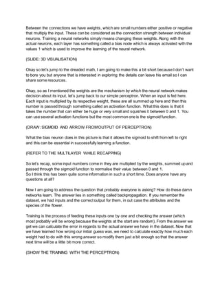
6. self.inNodes = inNodes + 1
self.outNodes = outNodes
self.alpha = alpha
# Matrix of weights init+ bias weight
self.weights = np.round(np.random.rand(self.inNodes,self.outNodes) - 0.5, 2)
def fwd (self,input):
# Add the bias value to the input
self.input= np.concatenate((input,[[1]]), axis=1)
# Sum the inputs and normalize for each output
sum = np.dot(self.input,self.weights)
self.output= SIG(sum)
return self.output
def bck (self,dL1):
# Derivative of L1 /w respectto the sum
dSIG_OUT = dSIG(self.output)
dL1_SUM = np.multiply(dL1,dSIG_OUT)
# Derivative of L1 /w respectto input (to be passed to L0)
W_T = np.transpose(self.weights)
dL1_L0 = np.dot(dL1_SUM,W_T)
dL1_L0 = np.delete(dL1_L0, -1,1)
# Change the weights using derivative of L1 /w respectto W
input_T= np.transpose(self.input)
dL1_W= np.dot(input_T,dL1_SUM)
self.weights -= self.alpha * dL1_W
return dL1_L0
class NeuralNetwork(object):
def __init__ (self,features,hiddenNeurons,classes,hiddenLayers = 1, alpha = 2):
# Create the first layer
self.layerStack = np.array([Layer(features,hiddenNeurons,alpha)])
# Create the hidden layers
for x in range(hiddenLayers - 1):
self.layerStack = np.append(self.layerStack,[Layer(hiddenNeurons,hiddenNeurons,

7. alpha)])
# Create the output layer
self.layerStack = np.append(self.layerStack,[Layer(hiddenNeurons,classes,alpha)])
np.set_printoptions(suppress=True,formatter={'float_kind':'{:f}'.format})
def eval(self,input):
# Forward the signal through the layers
lastInput= input
for l in self.layerStack:
lastInput= l.fwd(lastInput)
return lastInput
def train(self,input, target, iterations = 10000):
for i in range(iterations):
for j in range(input.shape[0]):
# For each inputvector in the data get the output
inputVector = input[j]
out = self.eval(inputVector)
# Get target value for training setand calc error
t = target[j]
errorVector = ERROR(t, out)
# Logging the error in the output
print(i, "t", np.sum(errorVector))
# Backpropagate the error though the layers
errorDerivative = dERROR(t, out)
for l in range(len(self.layerStack) -1, -1, -1):
errorDerivative = self.layerStack[l].bck(errorDerivative)