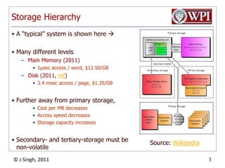
The document provides an overview and plan for a lecture on database management systems. Key points include: - By the second break, the lecture will cover storage hierarchies, secondary storage management, and system catalogs. - After the second break, the topics will include data modeling and storage hierarchies. - Storage hierarchies involve multiple storage levels from main memory to disk and beyond. The cost and performance of each level differs. - Techniques like caching aim to keep frequently used data in faster storage levels like memory.

1. CS 542 Database Management Systems J Singh March 14, 2011

2. Plan for today Putting it all together. Storage Hierarchy Secondary Storage Management System Catalogs By the second break, we will have arrived at a place where we have most of the tools to build our own database After the second break, Data Modeling This topic does not fit with the other three but some of you will need it for your project so I am including it

3. Storage Hierarchy A “typical” system is shown here  Many different levels Main Memory (2011) 1μsec access / word, $12.50/GB Disk (2011, ref) 3.4 msec access / page, $1.35/GB Further away from primary storage, Cost per MB decreases Access speed decreases Storage capacity increases Secondary- and tertiary-storage must be non-volatile Source: Wikipedia

4. DBMS vs. OS File System OS does disk space & buffer mgmt already So why not let OS manage these tasks? Differences in OS support: Portability issues Some limitations, e.g., files don’t span multiple disk devices. Buffer management in DBMS requires ability to: pin a page in buffer pool, force a page to disk (important for implementing CC & recovery), adjust replacement policy, and pre-fetch pages based on access patterns in typical DB operations.

5. Structure of a DBMS A typical DBMS has a layered architecture. Disk Storage hierarchy, RAID Disk Space Management Roles, Free blocks Buffer Management Buffer Pool, Replacement policy Files and Access Methods File organization heaps, sorted files, indexes File and Page level storage Query Optimization and Execution Relational Operators Files and Access Methods Buffer Management Disk Space Management DB These layers must consider concurrency control and recovery Index Files System Catalog Data Files

6. Five-minute rule (p1) Jim Gray, 1985, 1997 When it comes to improving database performance, Pay per MB when buying RAM If RAM is cheaper, we can afford to buy more Pay for speed when buying disk Faster disk, can get away with less RAM The critical question: At what point does the cost of keeping data in memory balance the cost of getting it from disk? Source: ACM Queue

7. Five-minute Rule (p2) In 1985 context: (ref) Block size: 1KB Disk: 15 I/Os per second = $15K 1 I/O per sec  $1K + overhead  $2K Memory $5K /MB  $5 /KB  1KB = $5 Trade-off Spend $5 for 1K in memory to save $2K in I/O cost? Sure! Any RAM cost up to $2K is good! $2K/$5 = 400 seconds Five minute rule: Have enough RAM to keep any data that will be used within 5 minutes In 1997 context: (ref) Re-validated and re-published In 2008 context: (ref) Still valid, but for much larger block sizes (64KB). Why? Disk speeds have not increased at the same rate as RAM capacity, making it more economical to bring in bigger blocks.

8. Extending the Hierarchy (p1) Flash memories (Solid-State Disks) (ref) Fit nicely at the half-way point between memory and disk 2011 price: 80¢/GB Persistent Storage Low Power Implications of 5-minute rule: RAM-Flash buffer size 4KB Flash-Disk buffer size 256KB Special uses? Index Structures? Materialized Views?

9. Extending the Hierarchy (P2) Principles of caching also extend into the cloud. Comparison: Disk (2011) 3.4 msec access, $1.35/GB Amazon S3 (2011) Highly Redundant storage constructed from cheap disks 100-250 msec access (across the network), $0.14/GB Potential Applications, How to turn a key-value store (e.g., Amazon SimpleDB) into a document store Use SimpleDB for its indexing capabilities Use S3 for storing documents Database backups / checkpoints into the cloud

10. Disks Secondary storage device of choice. Data is stored and retrieved in units: called disk blocks or pages. Unlike RAM, time to retrieve a disk page varies depending upon location on disk. Therefore, relative placement of pages on disk has major impact on DBMS performance

11. Components of a Disk Tracks Arm movement Arm assembly Spindle The platters spin. 15,000 rpm available 7,200 or 5,400 rpm are more typical The arm assembly is moved in or out to position a head on a desired track. Tracks under heads make a cylinder (imaginary!). Only one head reads/writes at any one time. Disk head Sector Platters Block size is a multiple of sector size (which is fixed).

12. Accessing a Disk Page Time to access (read/write) a disk block: seek time (moving arms to position disk head on track) rotational delay (waiting for block to rotate under head) transfer time (actually moving data to/from disk surface) Seek time and rotational delay dominate. Seek time varies from about 1 to 20msec Rotational delay varies from 0 to 10msec Transfer rate is about 1msec per 4KB page Lower I/O cost: reduce seek/rotation delays

13. Disk Access Optimizations Instead of responding to access requests in FIFO order, respond to them in an order that takes the disk characteristics into account Disk Scheduling Distribute data accesses among several disks and have them return data in parallel also known as Disk Striping Mirror disks Prefetch for sequential accesses Locate blocks strategically on disk to minimize seek times and rotational delay

14. Disk Scheduling Tracks Arm movement Arm assembly Spindle The Elevator Algorithm (like an elevator in a building) Sort all requests by cylinder outer to inner, Move arm inward and return results for each request Sort all requests inner to outer, Move arm outward and return results for each request Repeat Disk head Sector Platters

15. Disk Striping Distribute the data among several disks Seek time goes up, not down! But data transfer time can go down R1 R5 R9 R2 R6 R10 R3 R7 R11 R4 R8 R12

16. Mirror disks Can read from either copy, whichever is faster Must write to both copies Copy 1 Copy 2

17. Locating Blocks for Sequential access ‘Next’ block concept: blocks on same track, followed by blocks on same cylinder, followed by blocks on adjacent cylinder Blocks in a file should be arranged sequentially on disk (by `next’), to minimize seek and rotational delay. For a sequential scan, pre-fetching several pages at a time is a big win

18. CS-542 Database Management Systems Redundant Array of Independent Disks (RAID)

19. Introduction to RAID Arrangement of several disks that gives the abstraction of a single large disk Goals: Increase Performance and Reliability Techniques Data striping Data is partitioned Definition: size of each partition is called the striping unit Partitions are distributed over several disks Redundancy More disks  Increased reliability Redundant information allows reconstruction of data if disk fails

20. RAID Levels 0 and 1 Level 0: No redundancy Best write performance Not best in reading. (Why?) Level 1: Mirrored (two identical copies) Each disk has a mirror image Parallel reads, a write involves two disks. Maximum transfer rate = transfer rate of one disk

21. RAID Level 4 11110000 10101010 00111000 01100010 Arrangement Uses n data disks and 1 parity disk Block is striped across the n disks. The parity disk holds XOR of the blocks. Read: from the n data disks Write: update the data disks and also the parity disk Upon crash: remaining disks are used to reconstruct the data Problem: performance bottleneck on the parity disk

22. RAID Level 5 Arrangement 1/n of the cylinders of each disk are set aside for parity Thus the bottleneck is distributed evenly

23. Disk Space Management Lowest layer of DBMS software manages space on disk. Higher levels call upon this layer to: allocate/de-allocate a page read/write a page Higher levels don’t need to know how this is done, or how free space is managed.

24. Buffer Management in a DBMS DB Page Requests from Higher Levels BUFFER POOL disk page free frame MAIN MEMORY DISK choice of frame dictated by replacement policy Data must be in RAM for DBMS to operate on it! Table of <frame#, pageid> pairs is maintained.

25. When a Page is Requested ... If requested page is not in buffer pool: Choose a frame for replacement If frame is dirty, write it to disk Read requested page into chosen frame Pin the page and return its address. If requests can be predicted (e.g., sequential scans), pages can be pre-fetched

26. More on Buffer Management Requestor of page must unpin it, and indicate whether page has been modified: dirty bit is used for this. Page in pool may be requested many times, a pin count is used. A page is a candidate for replacement iffpin count = 0. CC & recovery may entail additional I/O when a frame is chosen for replacement. (Write-Ahead Log protocol; more later.)

27. Buffer Replacement Policy Frame is chosen for replacement by a replacement policy: Least-recently-used (LRU), Clock, MRU etc. Policy can have big impact on # of I/O’s; depends on access pattern. Sequential flooding: Nasty situation caused by LRU + repeated sequential scans. # buffer frames < # pages in file means each page request causes an I/O. MRU much better in this situation (but not in all situations, of course).

28. Representing addresses (p1) We need pointers especially in object oriented databases. Two kind of addresses: Physical (e.g. host, driveID, cylinder, surface, sector (block), offset) Logical (unique ID). Physical addresses are very long 8B is the minimum – up to 16B in some systems Example: A database that is designed to last 100 years. If the database grows to encompass 1 million machines and each machine creates 1 object each nanoseconds then we could have 277 objects. 10 bytes are needed to represent addresses for that many objects.

29. We need a map table for flexibility. The level of indirection gives the flexibility. For example, often we move records around, either within a block or from block to block. What about the programs that are pointing to these records? They are going to have dangling pointers, if they work with physical addresses. We only arrange the map table! physical logical Logical address Physical address Representing Addresses (p2)

30. Pointer Swizzling (p1) Typical DB structure: Data maintained by server process, using physical or logical addresses of perhaps 8 bytes. Application programs are clients with their own (conventional memory) address spaces. When blocks and records are copied to client's memory, DB addresses must be swizzled = translated to virtual­memory addresses. Allows conventional pointer following. Especially important in OODBMS, where pointers­as­dataare common. DBMS uses translation table Db address memory address

31. Pointer swizzling(p2) DBMS uses a translation table Map Table vs. Translation Table Logical and Physical address are both representations for the database address. In contrast, memory addresses in the translation table are for copies of the corresponding object in memory. All addressable items in the database have entries in the map table, while only those items currently in memory are mentioned in the translation table. Mem-addr DBaddr database address memory address

32. Swizzling Example Disk Memory Read into memory Swizzled Block 1 Unswizzled Block 2

33. Pointer Swizzling (p3) Swizzling Options: Never swizzle. Keep a translation table of DB pointers  local pointers; consult map to follow any DB pointer. Problem: time to follow pointers. Automatic swizzling. When a block is copied to memory, replace all its DB pointers by local pointers. Problem: requires knowing where every pointer is (use block and record headers for schema info). Problem: large investment if not too many pointer­followings occur. Swizzle on demand. When a block is copied to memory, enter its own address and those of member records into translation table, but do not translate pointers within the block. If we follow a pointer, translate it the first time. Problem: requires a bit in pointer fields for DB/local, Problem: extra decision at each pointer following.

34. Pinned records Pinned record = some swizzled pointer points to it Pointers to pinned records have to be unswizzled before the pinned record is returned to disk We need to know where the pointers to it are Implementation: keep a linked list of all (swizzled) records pointing to a record. y y x y Swizzled pointer

35. Variable-Length Data Skipped discussion of fixed-length records, please read in the book. Real complexity is with variable-length records Varying-size data items (e.g., address) Repeating fields (stars-to-movie relationship) Sliding Records Use offset table in a block, pointing to current records. If a record grows, slide records around the block. Not enough space? Create overflow block; offset table must indicate “record moved.”

37. Example: MySQL Information Schema INFORMATION_SCHEMA Tables The INFORMATION_SCHEMA SCHEMATA Table. The INFORMATION_SCHEMA TABLES Table. The INFORMATION_SCHEMA COLUMNS Table. The INFORMATION_SCHEMA STATISTICS Table. The INFORMATION_SCHEMA USER_PRIVILEGES Table. The INFORMATION_SCHEMA SCHEMA_PRIVILEGES Table. The INFORMATION_SCHEMA TABLE_PRIVILEGES Table. The INFORMATION_SCHEMA COLUMN_PRIVILEGES Table. The INFORMATION_SCHEMA CHARACTER_SETS Table … (Total 18 tables)

38. Summary Disks provide cheap, non-volatile storage. Random access, but cost depends on location of page on disk Important to arrange data sequentially to minimize seek and rotation delays. Buffer manager brings pages into RAM. Page stays in RAM until released by requestor. Written to disk when frame chosen for replacement. Frame to replace based on replacement policy. Tries to pre-fetch several pages at a time.

39. More Summary DBMS vs. OS File Support DBMS needs features not found in many OSs. forcing a page to disk controlling the order of page writes to disk files spanning disks ability to control pre-fetching and page replacement policy based on predictable access patterns Two mapping structures help us map addresses Map tables take us from logical addresses to physical addresses Translation tables take us from physical addresses to in-memory addresses (where applicable) Swizzling helps keep track of where in memory

40. Even More Summary Catalog relations store information about relations, indexes and views. Information common to all records in collection.

41. CS 542 – Database Management Systems Data Modeling

42. Data Modeling Techniques Entity-Relationship Modeling E/R Diagrams allow us to sketch database schema designs Designs are pictures called entity-relationship diagrams Weak Entity Sets Skipping, please read in book if interested, not on exam Converting E/R Diagrams to Relations Unified Modeling Language (UML) Skipping, please read in book if interested, not on exam Object Definition Language (ODL) Skipping, please read in book if interested, not on exam

43. Framework for E/R Design is a serious business. The “boss” (or customer) knows they want a database, but they don’t know what they want in it. Sketching the key components is an efficient way to develop a working database. 44

44. Entity Sets Entity = “thing” or object. Entity set = collection of similar entities. Similar to a class in object-oriented languages. Attribute= property of (the entities of) an entity set. Attributes are simple values, e.g. integers or character strings, not structs, sets, etc. In an entity-relationship diagram: Entity set = rectangle. Attribute = oval, with a line to the rectangle representing its entity set.

45. Example: Beer Manufacturers Entity set Beers has two attributes, name and manf (manufacturer). Each Beers entity has values for these two attributes, e.g. (Bud, Anheuser-Busch) name manf Beers

46. Relationships A relationship connects two or more entity sets. It is represented by a diamond, with lines to each of the entity sets involved. manf name name addr Sells Beers Bars Bars sell some beers. license Drinkers like some beers. Likes Frequents Note: license = beer, full, none Drinkers frequent some bars. Drinkers addr name

48. Example: 3-Way Relationship name addr name manf Bars Beers license Preferences Drinkers name addr

49. A Typical Relationship Set Each row of a relationship set typically consists of foreign keys to other tables

50. Many-Many Relationships Focus: binary relationships, such as Sells between Bars and Beers. In a many-many relationship, an entity of either set can be connected to many entities of the other set. E.g., a bar sells many beers; a beer is sold by many bars.

51. Many-One Relationships Some binary relationships are many -one from one entity set to another. Each entity of the first set is connected to at most one entity of the second set. But an entity of the second set can be connected to zero, one, or many entities of the first set. FavBeer, (Drinkers Beers) is many-one A drinker has at most one favBeer A beer can be the favorite of any number of drinkers, including zero

52. One-One Relationships In a one-one relationship, each entity of either entity set is related to at most one entity of the other set. Example: Relationship Best-seller between entity sets Manfs (manufacturer) and Beers. A beer cannot be made by more than one manufacturer No manufacturer can have more than one best-seller (assume no ties).

53. Representing “Multiplicity” Show a many-one relationship by an arrow entering the “one” side. Show a one-one relationship by arrows entering both entity sets. Rounded arrow = “exactly one,” i.e., each entity of the first set is related to exactly one entity of the target set.

54. Example: Many-One Relationship Likes Drinkers Beers Favorite Notice: two relationships connect the same entity sets, but are different.

55. Example: One-One Relationship Consider Best-seller between Manfs and Beers. But a beer manufacturer has to have a best-seller. Shown with a rounded arrow Some beers are not the best-seller of any manufacturer A rounded arrow to Manfs would be inappropriate A manufacturer has exactly one best seller. A beer is the best- seller for 0 or 1 manufacturer. Best- seller Manfs Beers

56. Attributes on Relationships Sometimes it is useful to attach an attribute to a relationship. Think of this attribute as a property of tuples in the relationship set. Sells Bars Beers price Price is a function of both the bar and the beer, not of one alone.

57. Subclasses in E/R Diagrams Subclass fewer entities, more properties. Example: Ales are a kind of beer. Not every beer is an ale, but some are. In addition to all the properties (attributes and relationships) of beers, suppose ales also have the attribute color. Assume subclasses form a tree. I.e., no multiple inheritance. Isa triangles indicate the subclass relationship. Beers name manf isa Ales color

58. E/R vs. Object-Oriented Subclasses Pete’s Ale In OO, objects are in one class only. Subclasses inherit from superclasses. In contrast, E/R entities have representatives in all subclasses to which they belong. Rule: if entity e is represented in a subclass, then e is represented in the superclass (and recursively up the tree). Beers name manf isa Ales color

59. Designating keys Show keys by underlining the attribute Beers name manf isa Ales color

60. 62 Example: Good name name addr ManfBy Beers Manfs This design gives the address of each manufacturer exactly once.

61. 63 Example: Bad name name addr ManfBy Beers Manfs manf This design states the manufacturer of a beer twice: as an attribute and as a related entity.

62. 64 Example: Bad name manf manfAddr Beers This design repeats the manufacturer’s address once for each beer and loses the address if there are temporarily no beers for a manufacturer.

63. Example: Good name name addr ManfBy Beers Manfs Manfs deserves to be an entity set because of the nonkey attribute addr. Beers deserves to be an entity set because it is the “many” of the many-one relationship ManfBy.

65. Entity Set Relation Relation: Beers(name, manf) name manf Beers 68

66. Relationship Relation Likes 2 1 Favorite Buddies Likes(drinker, beer) Favorite(drinker, beer) wife husband Buddies(name1, name2) Married Married(husband, wife) name name addr manf Drinkers Beers

67. Combining Relations OK to combine into one relation: The relation for an entity-set E The relations for many-one relationships of which E is the “many.” Example: Drinkers(name, addr) and Favorite(drinker, beer) combine to make Drinker1(name, addr, favBeer).

68. Risk with Many-Many Relationships Combining Drinkers with Likes would be a mistake. It leads to redundancy, as: Redundancy name addr beer Sally 123 Maple Bud Sally 123 Maple Miller

69. Subclasses: Three Approaches Object-oriented: One relation per subset of subclasses, with all relevant attributes. Use nulls: One relation; entities have NULL in attributes that don’t belong to them. E/R style: One relation for each subclass: Key attribute(s). Attributes of that subclass. 72

70. Example: Subclass Relations Beers name manf isa Ales color

71. Object-Oriented Beers Ales Good for queries like “find the color of ales made by Pete’s” Beers name manf isa Ales color

72. E/R Style Beers Ales Good for queries like “find all beers, including ales, made by Pete’s” Beers name manf isa Ales color

73. Using NULLS Beers Saves space and does everything with one table Beers name manf isa Ales color

74. Data Models forNoSQL Databases Class Discussion at Next Meeting. How would you represent a many-to-many relationships in? Amazon SimpleDB? Cassandra? Google App Engine? MongoDB? Redis? Other? Inviting a 3-minute presentation (on 3/21) for 20 bonus points Only one presentation per DB Please volunteer by Tuesday noon if interested I will let you know by Wednesday noon if you were selected

75. Summary Data Modeling is an essential part of designing an application Intersects business and technology Essential elements Entities Relationships Is-a relationships Multiplicity Has to be done with an eye toward the long term (But has to avoid analysis paralysis) Attributes can be added later but Entities and Relationships are baked-in in the beginning and very hard to change later Pay particular attention to multiplicity of relationships Best to separate modeling from “table design” Needed for all databases, Relational or not.

76. Next meetings March21: Sort and Join Processing Sort: Chapter 15 Join: Sections 16.1 – 16.4