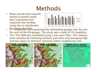
Melissa Slater, Josh Roberti, Chris Daly, Stephanie Laseter, Lloyd Swift,
Adam Skibbe
Overview
• Data
• Methods
• Statistical
Analysis
• Results
Purpose
This study examines the spatial
distribution of mean annual and seasonal
(winter/summer) precipitation readings
collected from sixty-nine gauges within
the forest from 1951 to 1958.
The intent was to evaluate the relationship
between elevation and precipitation,
identify an optimal scale and interpolation
model, and quantify spatial uncertainty by
cross-validating the interpolated results
against observed data.
Data
• 69 gauges recorded
continuous precipitation
measurements from 1951-
1958. This is the longest
continuous record with the
largest number of fully
functioning gauges.
• A 1/3 arc-second Digital
Elevation Model from the USGS
National Elevation Dataset
provided the base elevations
for the 69 gauges.
• The Coweeta Creek – Little
Tennessee River watershed of
the Coweeta basin provided
the extent for the
interpolation models.
• The 1983 North American
Datum was utilized.
• A local Universal Transverse
Mercator projection for Zone
17 North was applied.
Methods
• n-1 shapefiles were generated by eliminating gauges one-by-one
for each of the 69 gauges. The result was a total of 70 shapefiles.
• The 10m DEM was smoothed using a low-pass filter. This reduces
local variation by removing artifacts and noise and averaging high
and low values to diminish extremes within neighboring cells.
• Mean annual and seasonal
(winter/summer) totals
were calculated then
imported into ArcMap
using the xy coordinates
for gauge locations.
Methods Continued
• A Focal Statistics tool was then applied to the filtered DEM to
smooth the grid and generate additional scales from 100-
10,000 meter resolution.
• Extract Values to Points was used to derive elevation values
(z) at each gauge location for each DEM scale.
• Ordinary Least Squares (OLS) linear regression script was run
using derived elevation values and actual precipitation values
on the X/Y axes.
Methods Continued
• The coefficient of determination was examined along with the
scatterplots produced from the OLS regression to determine optimal
scale for modeling precipitation in the Coweeta Experimental Forest.
• At 7,000 m
the R² for
the Annual
and
Seasonal
values
showed that
approximat
ely81-95%
of
prediction
errors could
be reduced.
Methods Continued
• A Pivot Table model was run to extract the coefficient values from
the optimal 7,000 meter DEM.
• A Raster Calculation was performed with the regression function to
create an “initial” precipitation grid.
• IDW and Kriged
interpolation methods
were run on the
residuals produced
from the regression
analysis with various
neighborhood and
power settings adjusted
to obtain the optimal
modeling parameters.
Methods Concluded
• A batch Raster Calculation was used to add the interpolated residual
grids to the “initial” precipitation grids to generate a set of “final”
precipitation grids.
• Extract Values to Points was run again to extract the predicted
precipitation values from each of the final grids.
Statistical Analysis
• Signed error (residual bias = observed – predicted) was calculated
along with the unsigned Mean Absolute Error (%MAE =
((abs([bias])/observed)*100)) for the annual and seasonal values.
• Mean predicted and
observed values, mean
bias, %MAE, root mean
square error and the
standard deviation for the
mean absolute error,
predicted, observed and
biased results were
calculated.
Results
• Elevation explains a majority of the spatial
patterns of precipitation with in the
Coweeta Experimental Forest and varies
with season.
• A 7000-m effective resolution DEM
produced statistically improved results,
showing that the dominant scale of
orographic processes is relatively large.
• The Kriged residual interpolation performed
better than the IDW model.
Next Steps
• These high-quality precipitation maps can
serve as “ground truth” for quantifying
uncertainty in US-wide spatial precipitation
products used in a large number of
hydrologic and ecological applications.
• The uncertainty in
PRISM US-wide
precipitation grids
will be evaluated
and sources of
error identified,
including the
effects of coarse
Questions?
Acknowledgements
• Josh Roberti – The National Ecological Observatory
Network
• Chris Daly – The PRISM Climate Group, Oregon State
University
• Jeff Taylor – Aspen Global Change Institute
• Lloyd Swift – US Forest Service, Coweeta Hydrological
Laboratory
• Stephanie Laseter – US Forest Service, Coweeta
Hydrological Laboratory
• Ruth D Yanai – College of Environmental Science and
Forestry, State University of New York
• Chelcy Ford Miniat – US Forest Service, Coweeta
Hydrological Laboratory
• Adam Skibbe – Department of Geographical and
Sustainability Sciences, University of Iowa

Coweeta ppt cd_ms

  • 1.
    Melissa Slater, JoshRoberti, Chris Daly, Stephanie Laseter, Lloyd Swift, Adam Skibbe
  • 2.
    Overview • Data • Methods •Statistical Analysis • Results
  • 4.
    Purpose This study examinesthe spatial distribution of mean annual and seasonal (winter/summer) precipitation readings collected from sixty-nine gauges within the forest from 1951 to 1958. The intent was to evaluate the relationship between elevation and precipitation, identify an optimal scale and interpolation model, and quantify spatial uncertainty by cross-validating the interpolated results against observed data.
  • 5.
    Data • 69 gaugesrecorded continuous precipitation measurements from 1951- 1958. This is the longest continuous record with the largest number of fully functioning gauges. • A 1/3 arc-second Digital Elevation Model from the USGS National Elevation Dataset provided the base elevations for the 69 gauges. • The Coweeta Creek – Little Tennessee River watershed of the Coweeta basin provided the extent for the interpolation models. • The 1983 North American Datum was utilized. • A local Universal Transverse Mercator projection for Zone 17 North was applied.
  • 6.
    Methods • n-1 shapefileswere generated by eliminating gauges one-by-one for each of the 69 gauges. The result was a total of 70 shapefiles. • The 10m DEM was smoothed using a low-pass filter. This reduces local variation by removing artifacts and noise and averaging high and low values to diminish extremes within neighboring cells. • Mean annual and seasonal (winter/summer) totals were calculated then imported into ArcMap using the xy coordinates for gauge locations.
  • 7.
    Methods Continued • AFocal Statistics tool was then applied to the filtered DEM to smooth the grid and generate additional scales from 100- 10,000 meter resolution. • Extract Values to Points was used to derive elevation values (z) at each gauge location for each DEM scale. • Ordinary Least Squares (OLS) linear regression script was run using derived elevation values and actual precipitation values on the X/Y axes.
  • 8.
    Methods Continued • Thecoefficient of determination was examined along with the scatterplots produced from the OLS regression to determine optimal scale for modeling precipitation in the Coweeta Experimental Forest. • At 7,000 m the R² for the Annual and Seasonal values showed that approximat ely81-95% of prediction errors could be reduced.
  • 9.
    Methods Continued • APivot Table model was run to extract the coefficient values from the optimal 7,000 meter DEM. • A Raster Calculation was performed with the regression function to create an “initial” precipitation grid. • IDW and Kriged interpolation methods were run on the residuals produced from the regression analysis with various neighborhood and power settings adjusted to obtain the optimal modeling parameters.
  • 10.
    Methods Concluded • Abatch Raster Calculation was used to add the interpolated residual grids to the “initial” precipitation grids to generate a set of “final” precipitation grids. • Extract Values to Points was run again to extract the predicted precipitation values from each of the final grids.
  • 11.
    Statistical Analysis • Signederror (residual bias = observed – predicted) was calculated along with the unsigned Mean Absolute Error (%MAE = ((abs([bias])/observed)*100)) for the annual and seasonal values. • Mean predicted and observed values, mean bias, %MAE, root mean square error and the standard deviation for the mean absolute error, predicted, observed and biased results were calculated.
  • 12.
    Results • Elevation explainsa majority of the spatial patterns of precipitation with in the Coweeta Experimental Forest and varies with season. • A 7000-m effective resolution DEM produced statistically improved results, showing that the dominant scale of orographic processes is relatively large. • The Kriged residual interpolation performed better than the IDW model.
  • 13.
    Next Steps • Thesehigh-quality precipitation maps can serve as “ground truth” for quantifying uncertainty in US-wide spatial precipitation products used in a large number of hydrologic and ecological applications. • The uncertainty in PRISM US-wide precipitation grids will be evaluated and sources of error identified, including the effects of coarse
  • 14.
  • 15.
    Acknowledgements • Josh Roberti– The National Ecological Observatory Network • Chris Daly – The PRISM Climate Group, Oregon State University • Jeff Taylor – Aspen Global Change Institute • Lloyd Swift – US Forest Service, Coweeta Hydrological Laboratory • Stephanie Laseter – US Forest Service, Coweeta Hydrological Laboratory • Ruth D Yanai – College of Environmental Science and Forestry, State University of New York • Chelcy Ford Miniat – US Forest Service, Coweeta Hydrological Laboratory • Adam Skibbe – Department of Geographical and Sustainability Sciences, University of Iowa

Editor's Notes

  • #3 How well does interpolation represent actual rainfall accumulation?
  • #4 The Coweeta Experimental forest is located south western North Carolina in the Nan ta hala Mountain range of the southern Appalachians. Established in 1933 as a long-term watershed management study, the Coweeta Experimental Forest holds some of the longest continuous environmental studies in the U.S and is one of the oldest gauged watershed sites in the world. The watershed used in this study encompasses about 16 square km across an elevation gradient of approximately 1000 meters.
  • #5 The purpose was to examine the spatial distribution of annual and seasonal readings collected from 69 gauges within the forest over an 8 year study period from 1951 to 1958. The intent was multi-faceted; The first was to examine the relationship between elevation and precipitation Next, identify an optimal scale Third identify an optimal interpolation model, And then quantify spatial uncertainty by cross-validating the interpolated results against observed data.
  • #6 The 69 gauges utilized in this study recorded continuous precipitation measurements from 1951 to 1958 and is the longest continuous record with the largest number of fully functioning gauges.
  • #9 The regression analysis produced a variety of outputs but we first looked to the scatterplots and the coefficients of determination to determine the optimal scale. At 10 meters the relationship between elevation and precipitation is positive and moderate with 48 to 64% of errors explained when elevation is taken into account. As we scaled up, that relationship strength continued to increase and at 7000 meters 81-95% of prediction errors could be reduced. While r squared valued beyond 7,000 meters were still exceptionally good they did start to decline slightly and so it was determined that 7000 meters was the optimal scale for this project. The remaining methods were run against the 7000 meter DEM
  • #10 A pivot table model was run to extract the slope and intercept values from the coefficient tables produced from the OLS regression. These values were then applied to the DEM as a regression line equation using a raster calculation mode. The output resulted in an initial set of precipitation grids. Next I ran the interpolation on the residuals produced from the OLS regression. In order to ascertain the optimal model parameters IDW and Kriged interpolations were iterated through using a search radius of 12 to 30 neighbors for the annual and seasonal values. The outputs were analyzed by looking at the residual sum, average residual bias and the percent mean absolute error. The Kriged model showed statistical improvement when using a search radius of 24 neighboring input points but since IDW is an exact interpolator meaning that minimum and maximum values can only occur at the sample location the change of neighboring input points did not significantly impact the statistical output. The default value of 12 neighbors was used in the IDW model. One other parameter I looked at for IDW was the power function which was run with the default setting of 2 and then adjusted to 1 to increase the distance of influence and attempt to smooth the surface. The statistical outputs showed that the default power setting of 2 produced slightly higher results for the % MAE but lower results for both the residual sum and the average residual bias indicating that overall the default power was a statistically smoother model.
  • #11 The final steps were to add the interpolated grids to the initial grids and creat a set of final precipitation girds. The extract values to points model was run again to extract the predicted precipitation for each of the final grids.
  • #12 Next, statistical analysis was run to evaluate the signed error or residual bias (observed – predicted) along with the unsigned Mean Absolute Error or %MAE ((abs([bias])/observed)*100). Additional statistical calculations included mean predicted and observed values, mean bias, mean percent absolute error, root mean square error and the standard deviation for the mean absolute error, predicted, observed and biased results.   Next, in order to quantify the results from the exact and deterministic interpolation models, boxplots were generated to examine the difference in predicted vs observed values for the winter, summer, and annual means Another boxplot was generated to examine the difference in the seasonal and annual % Mean Average Error between the two interpolation models Although the IDW model is an exact interpolator The Kriged model showed a smaller range of %MAE and average bias compared to the IDW model indicating less deviation from predicted values.
  • #13 As expected, elevation explains a majority of the spatial patterns of precipitation within the Coweeta Experimental Forest and the smoother resolution of 7,000 meters produced statistically improved results. Upon examination of the n-1 cross-validation models the spread between the minimum and maximum values of the predicted locations were larger than the observed values in the IDW model but observed maximum values were larger in the Kriged model. The Kriged model shows a smaller range of %MAE and average bias compared to the IDW model. The IDW model shows greater mean and standard deviation values when compared to the Kriged model. The percent mean absolute error for the interpolation models ranged from 1.6-3.2% with a root mean square error of less than 62 mm (>2.5 inches). Ultimately the Kriged model had less deviation from predicted values than the IDW model. While a statistical approach is valuable in terms of repeatability, economic viability and speed, unfortunately, cross-validation has its limitations and the measurement of error is only applicable to locations with existing data. Being able to quantify uncertainties and determine a threshold for acceptable error proves to be challenging. Understanding the orographic features within a study area and the local variables that affect the data, as well optimizing the layout of collection networks and utilizing proper modeling parameters can help significantly reduce spatial uncertainty.
  • #14 As expected, elevation explains a majority of the spatial patterns of precipitation within the Coweeta Experimental Forest and the smoother resolution of 7,000 meters produced statistically improved results. Upon examination of the n-1 cross-validation models the spread between the minimum and maximum values of the predicted locations were larger than the observed values in the IDW model but observed maximum values were larger in the Kriged model. The Kriged model shows a smaller range of %MAE and average bias compared to the IDW model. The IDW model shows greater mean and standard deviation values when compared to the Kriged model. The percent mean absolute error for the interpolation models ranged from 1.6-3.2% with a root mean square error of less than 62 mm (>2.5 inches). Ultimately the Kriged model had less deviation from predicted values than the IDW model. While a statistical approach is valuable in terms of repeatability, economic viability and speed, unfortunately, cross-validation has its limitations and the measurement of error is only applicable to locations with existing data. Being able to quantify uncertainties and determine a threshold for acceptable error proves to be challenging. Understanding the orographic features within a study area and the local variables that affect the data, as well optimizing the layout of collection networks and utilizing proper modeling parameters can help significantly reduce spatial uncertainty.