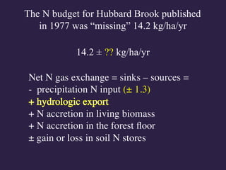
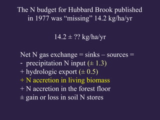
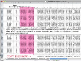
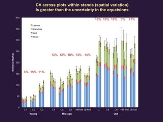
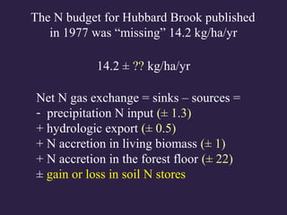
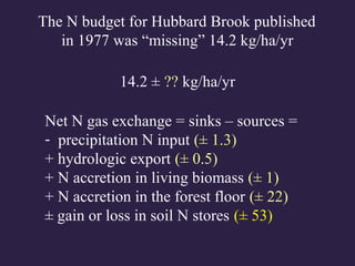
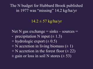
ESA 2014 Workshop 18
Tools for Estimating
Uncertainty in Ecology
Ruth D. Yanai
State University of New York
College of Environmental Science and Forestry
Syracuse NY 13210, USA
Quantifying uncertainty in ecosystem budgets
Precipitation (evaluating monitoring intensity)
Streamflow (filling gaps with minimal uncertainty)
Forest biomass (identifying the greatest sources of uncertainty)
Soil stores, belowground carbon turnover (detectable differences)
QUANTIFYING UNCERTAINTY
IN ECOSYSTEM STUDIES
UNCERTAINTY
Natural Variability
Spatial Variability
Temporal Variability
Knowledge Uncertainty
Measurement Error
Model Error
Types of uncertainty commonly
encountered in ecosystem studies
Adapted from Harmon et al. (2007)
Bormann et al. (1977) Science
How can we assign confidence in ecosystem
nutrient fluxes?
Bormann et al. (1977) Science
The N budget for Hubbard Brook published
in 1977 was “missing” 14.2 kg/ha/yr
Net N gas exchange = sinks – sources =
- precipitation N input
+ hydrologic export
+ N accretion in living biomass
+ N accretion in the forest floor
± gain or loss in soil N stores
- weathering N input
The N budget for Hubbard Brook published
in 1977 was “missing” 14.2 kg/ha/yr
14.2 ± ?? kg/ha/yr
The N budget for Hubbard Brook published
in 1977 was “missing” 14.2 kg/ha/yr
14.2 ± ?? kg/ha/yr
Measurement Uncertainty Sampling Uncertainty
Spatial and Temporal Variability
Model Uncertainty
Error within models Error between models
Volume = f(elevation, aspect): 3.4 mm
Undercatch: 3.5%
Chemical analysis: 0-3%
Model selection: <1%
Across
catchments:
3%
Across years:
14%
We tested the effect of sampling intensity by sequentially omitting
individual precipitation gauges.
Estimates of annual precipitation volume varied little until five or more
of the eleven precipitation gauges were ignored.
The N budget for Hubbard Brook published
in 1977 was “missing” 14.2 kg/ha/yr
14.2 ± ?? kg/ha/yr
The N budget for Hubbard Brook published
in 1977 was “missing” 14.2 kg/ha/yr
14.2 ± ?? kg/ha/yr
Don Buso HBES
Gaps in the discharge record are filled by
comparison to other streams at the site,
using linear regression.
S5
S12
S16
S17
S20
0
100
200
0 100 200
0
100
200
300
0 100 200 300
0
50
100
150
0 50 100 150
0
50
100
150
0 50 100 150
0
50
100
0 50 100
Cross-validation: Create fake gaps and
compare observed and predicted discharge
Net N gas exchange = sinks – sources =
- precipitation N input (± 1.3)
+ hydrologic export (± 0.5)
+ N accretion in living biomass
+ N accretion in the forest floor
± gain or loss in soil N stores
The N budget for Hubbard Brook published
in 1977 was “missing” 14.2 kg/ha/yr
14.2 ± ?? kg/ha/yr
Net N gas exchange = sinks – sources =
- precipitation N input (± 1.3)
+ hydrologic export (± 0.5)
+ N accretion in living biomass
+ N accretion in the forest floor
± gain or loss in soil N stores
The N budget for Hubbard Brook published
in 1977 was “missing” 14.2 kg/ha/yr
14.2 ± ?? kg/ha/yr
Monte Carlo
Simulation
Yanai, Battles, Richardson, Rastetter,
Wood, and Blodgett (2010) Ecosystems
Monte Carlo simulations use
random sampling of the
distribution of the inputs to a
calculation. After many
iterations, the distribution of the
output is analyzed.
A Monte-Carlo approach could be
implemented using specialized software or
almost any programming language.
Here we used a spreadsheet model.
Height Parameters
Height = 10^(a + b*log(Diameter) + log(E))
Lookup
Lookup
Lookup
***IMPORTANT***
Random selection of parameter values
happens HERE, not separately for each tree
If the errors were sampled
individually for each tree,
they would average out to
zero by the time you added
up a few thousand trees
Biomass Parameters
Biomass = 10^(a + b*log(PV) + log(E))
Lookup
Lookup
Lookup
PV = 1/2 r2
* Height
Biomass Parameters
Biomass = 10^(a + b*log(PV) + log(E))
Lookup
Lookup
Lookup
PV = 1/2 r2
* Height
Biomass Parameters
Biomass = 10^(a + b*log(PV) + log(E))
Lookup
Lookup
Lookup
PV = 1/2 r2
* Height
Concentration Parameters
Concentration = constant + error
Lookup
Lookup
COPY THIS ROW-->
After enough
interations, analyze
your results
Paste Values button
C1 C2 C3 C4 C5 C6 HB-Mid JB-Mid C7 C8 C9 HB- Old JB-Old
Young Mid-Age Old
Biomass of thirteen stands
of different ages
C1 C2 C3 C4 C5 C6 HB-Mid JB-Mid C7 C8 C9 HB- Old JB-Old
3% 7% 3%
4% 4% 3% 3% 3%
3% 2% 4% 4% 5%
Coefficient of variation (standard deviation / mean)
of error in allometric equations
Young Mid-Age Old
C1 C2 C3 C4 C5 C6 HB-Mid JB-Mid C7 C8 C9 HB- Old JB-Old
Young Mid-Age Old
3% 7% 3%
4% 4% 3% 3% 3%
3% 2% 4% 4% 5%
CV across plots within stands (spatial variation)
Is greater than the uncertainty in the equatsions
6% 15% 11%
12% 12% 18% 13% 14%
16% 10% 19% 3% 11%
“What is the greatest source of
uncertainty in my answer?”
Better than the sensitivity estimates that
vary everything by the same amount--
they don’t all vary by the same amount!
Better than the uncertainty in the
parameter estimates--we can tolerate a
large uncertainty in an unimportant
parameter.
“What is the greatest source of
uncertainty to my answer?”
0
20
40
60
80
100
120
Stem
Wood
Stem
Bark
Branches Leaves Twigs Roots Light
Wood
Dark
Wood
Tissue
Biomass (Mg/ha)
0%
5%
10%
15%
20%
25%
30%
35%
40%
45%
50%
Stem
Wood
Stem
Bark
Branches Leaves Twigs Roots Light
Wood
Dark
Wood
Tissue
CV of Biomass
0
5
10
15
20
25
Stem
Wood
Stem
Bark
Branches Leaves Twigs Roots Light
Wood
Dark
Wood
Tissue
Biomass Standard Deviation
(Mg/ha)
0
50
100
150
200
250
Stem Bark Branches Leaves Twigs Roots Light
Wood
Dark wood
Tissue
N content (kg/ha)
0%
5%
10%
15%
20%
25%
30%
35%
40%
45%
50%
Stem Bark Branches Leaves Twigs Roots Light
Wood
Dark wood
Tissue
CV of N Content
0
10
20
30
40
50
60
70
80
90
100
Stem Bark Branches Leaves Twigs Roots Light
Wood
Dark wood
Tissue
N Content Standard Deviation
(kg/ha)
Net N gas exchange = sinks – sources =
- precipitation N input (± 1.3)
+ hydrologic export (± 0.5)
+ N accretion in living biomass (± 1)
+ N accretion in the forest floor
± gain or loss in soil N stores
The N budget for Hubbard Brook published
in 1977 was “missing” 14.2 kg/ha/yr
14.2 ± ?? kg/ha/yr
Net N gas exchange = sinks – sources =
- precipitation N input (± 1.3)
+ hydrologic export (± 0.5)
+ N accretion in living biomass (± 1)
+ N accretion in the forest floor
± gain or loss in soil N stores
The N budget for Hubbard Brook published
in 1977 was “missing” 14.2 kg/ha/yr
14.2 ± ?? kg/ha/yr
Oi
Oe
Oa
E
Bh
Bs
Forest
Floor
Mineral
Soil
}
}
Nitrogen in the Forest Floor
Hubbard Brook Experimental Forest
y = 0.0002x - 0.1619
R
2
= 0.0109
0
0.05
0.1
0.15
0.2
0.25
1975 1980 1985 1990 1995 2000 2005
Forest Floor N (kg/m2)
Nitrogen in the Forest Floor
Hubbard Brook Experimental Forest
y = 0.0002x - 0.1619
R
2
= 0.0109
0
0.05
0.1
0.15
0.2
0.25
1975 1980 1985 1990 1995 2000 2005
Forest Floor N (kg/m2)
The change is insignificant (P = 0.84).
The uncertainty in the slope is ± 22 kg/ha/yr.
Net N gas exchange = sinks – sources =
- precipitation N input (± 1.3)
+ hydrologic export (± 0.5)
+ N accretion in living biomass (± 1)
+ N accretion in the forest floor (± 22)
± gain or loss in soil N stores
The N budget for Hubbard Brook published
in 1977 was “missing” 14.2 kg/ha/yr
14.2 ± ?? kg/ha/yr
Nitrogen Pools (kg/ha)
Hubbard Brook Experimental Forest
1796
29
10
1260
750
3080
Forest Floor
Live Vegetation
Coarse Woody Debris
Mineral Soil
10 cm-C
Dead Vegetation
Mineral Soil
0-10 cm
We can’t detect a difference of 730 kg N/ha in the mineral soil.
From 1983 to 1998, 15 years post-harvest, there was an
insignificant decline of 54 ± 53 kg N ha-1
y-1
Huntington et al. (1988)
Net N gas exchange = sinks – sources =
- precipitation N input (± 1.3)
+ hydrologic export (± 0.5)
+ N accretion in living biomass (± 1)
+ N accretion in the forest floor (± 22)
± gain or loss in soil N stores (± 53)
The N budget for Hubbard Brook published
in 1977 was “missing” 14.2 kg/ha/yr
14.2 ± ?? kg/ha/yr
Net N gas exchange = sinks – sources =
- precipitation N input (± 1.3)
+ hydrologic export (± 0.5)
+ N accretion in living biomass (± 1)
+ N accretion in the forest floor (± 22)
± gain or loss in soil N stores (± 53)
The N budget for Hubbard Brook published
in 1977 was “missing” 14.2 kg/ha/yr
14.2 ± 57 kg/ha/yr
Measurement Uncertainty Sampling Uncertainty
Spatial Variability
Model Uncertainty y
Error within models Error between models
Excludes areas not sampled: rock area 5%, stem area: 1%
Measurement uncertainty and spatial variation make it difficult
to estimate soil carbon and nutrient contents precisely
Studies of soil change over time often fail to detect a difference.
We should always report how large a difference is detectable.
Yanai et al. (2003) SSSAJ
Power analysis can be used to determine the
difference detectable with known confidence
Sampling the same experimental units over time
permits detection of smaller changes
In this analysis of forest floor studies,
few could detect small changes
Yanai et al. (2003) SSSAJ
The Value of Uncertainty Analysis
Quantify uncertainty in our results
Uncertainty in regression
Monte Carlo sampling
Detectable differences
Identify ways to reduce uncertainty
Devote effort to the greatest unknowns
Improve efficiency of monitoring efforts
Be a part of QUEST!
• Find more information at: www.quantifyinguncertainty.org
• Read papers, share sample code, stay updated with QUEST News
• Email us at quantifyinguncertainty@gmail.com
• Follow us on LinkedIn and Twitter: @QUEST_RCN
QUANTIFYING UNCERTAINTY
IN ECOSYSTEM STUDIES
References
Yanai, R.D., C.R. Levine, M.B. Green, and J.L. Campbell. 2012. Quantifying
uncertainty in forest nutrient budgets, J. For. 110: 448-456
Yanai, R.D., J.J. Battles, A.D. Richardson, E.B. Rastetter, D.M. Wood, and C.
Blodgett. 2010. Estimating uncertainty in ecosystem budget calculations.
Ecosystems 13: 239-248
Wielopolski, L, R.D. Yanai, C.R. Levine, S. Mitra, and M.A Vadeboncoeur.
2010. Rapid, non-destructive carbon analysis of forest soils using neutron-
induced gamma-ray spectroscopy. For. Ecol. Manag. 260: 1132-1137
Park, B.B., R.D. Yanai, T.J. Fahey, T.G. Siccama, S.W. Bailey, J.B. Shanley,
and N.L. Cleavitt. 2008. Fine root dynamics and forest production across a
calcium gradient in northern hardwood and conifer ecosystems. Ecosystems
11:325-341
Yanai, R.D., S.V. Stehman, M.A. Arthur, C.E. Prescott, A.J. Friedland, T.G.
Siccama, and D. Binkley. 2003. Detecting change in forest floor carbon. Soil
Sci. Soc. Am. J. 67:1583-1593
My web site: www.esf.edu/faculty/yanai (Download any papers)
Alternative spatial models for precipitation in the Hubbard Brook Valley
0.36%
0.58%
0.24%
0.77% 0.83%
Monte Carlo
Simulation
Yanai, Battles, Richardson, Rastetter,
Wood, and Blodgett (2010) Ecosystems
Monte Carlo simulations use
random sampling of the
distribution of the inputs to a
calculation. After many
iterations, the distribution of the
output is analyzed.
Repeated Calculations of N in Biomass
Hubbard Brook Watershed 6
611 ± 54 kg N/ha
Nitrogen Content of Biomass
with Uncertainty
***IMPORTANT***
Random selection of parameter
values applies across all time
periods in each iteration.
The uncertainty between two
measurements can be less than
in a single measurement!
100 Simultaneous Calculations
of N in Biomass in 1997 and 2002
100 Simultaneous Calculations
of N in Biomass in 1997 and 2002
Accumulation Rate of N in Biomass
Distribution of Estimates
± 5 kg N/ha over 5 yr

Yanai esa workshop 2014

  • 1.
    ESA 2014 Workshop18 Tools for Estimating Uncertainty in Ecology Ruth D. Yanai State University of New York College of Environmental Science and Forestry Syracuse NY 13210, USA
  • 2.
    Quantifying uncertainty inecosystem budgets Precipitation (evaluating monitoring intensity) Streamflow (filling gaps with minimal uncertainty) Forest biomass (identifying the greatest sources of uncertainty) Soil stores, belowground carbon turnover (detectable differences) QUANTIFYING UNCERTAINTY IN ECOSYSTEM STUDIES
  • 3.
    UNCERTAINTY Natural Variability Spatial Variability TemporalVariability Knowledge Uncertainty Measurement Error Model Error Types of uncertainty commonly encountered in ecosystem studies Adapted from Harmon et al. (2007)
  • 4.
    Bormann et al.(1977) Science How can we assign confidence in ecosystem nutrient fluxes?
  • 5.
    Bormann et al.(1977) Science The N budget for Hubbard Brook published in 1977 was “missing” 14.2 kg/ha/yr
  • 6.
    Net N gasexchange = sinks – sources = - precipitation N input + hydrologic export + N accretion in living biomass + N accretion in the forest floor ± gain or loss in soil N stores - weathering N input The N budget for Hubbard Brook published in 1977 was “missing” 14.2 kg/ha/yr 14.2 ± ?? kg/ha/yr
  • 7.
    The N budgetfor Hubbard Brook published in 1977 was “missing” 14.2 kg/ha/yr 14.2 ± ?? kg/ha/yr
  • 8.
    Measurement Uncertainty SamplingUncertainty Spatial and Temporal Variability Model Uncertainty Error within models Error between models Volume = f(elevation, aspect): 3.4 mm Undercatch: 3.5% Chemical analysis: 0-3% Model selection: <1% Across catchments: 3% Across years: 14%
  • 10.
    We tested theeffect of sampling intensity by sequentially omitting individual precipitation gauges. Estimates of annual precipitation volume varied little until five or more of the eleven precipitation gauges were ignored.
  • 11.
    The N budgetfor Hubbard Brook published in 1977 was “missing” 14.2 kg/ha/yr 14.2 ± ?? kg/ha/yr
  • 12.
    The N budgetfor Hubbard Brook published in 1977 was “missing” 14.2 kg/ha/yr 14.2 ± ?? kg/ha/yr
  • 14.
  • 15.
    Gaps in thedischarge record are filled by comparison to other streams at the site, using linear regression. S5 S12 S16 S17 S20 0 100 200 0 100 200 0 100 200 300 0 100 200 300 0 50 100 150 0 50 100 150 0 50 100 150 0 50 100 150 0 50 100 0 50 100
  • 16.
    Cross-validation: Create fakegaps and compare observed and predicted discharge
  • 17.
    Net N gasexchange = sinks – sources = - precipitation N input (± 1.3) + hydrologic export (± 0.5) + N accretion in living biomass + N accretion in the forest floor ± gain or loss in soil N stores The N budget for Hubbard Brook published in 1977 was “missing” 14.2 kg/ha/yr 14.2 ± ?? kg/ha/yr
  • 18.
    Net N gasexchange = sinks – sources = - precipitation N input (± 1.3) + hydrologic export (± 0.5) + N accretion in living biomass + N accretion in the forest floor ± gain or loss in soil N stores The N budget for Hubbard Brook published in 1977 was “missing” 14.2 kg/ha/yr 14.2 ± ?? kg/ha/yr
  • 19.
    Monte Carlo Simulation Yanai, Battles,Richardson, Rastetter, Wood, and Blodgett (2010) Ecosystems Monte Carlo simulations use random sampling of the distribution of the inputs to a calculation. After many iterations, the distribution of the output is analyzed.
  • 20.
    A Monte-Carlo approachcould be implemented using specialized software or almost any programming language. Here we used a spreadsheet model.
  • 21.
    Height Parameters Height =10^(a + b*log(Diameter) + log(E)) Lookup Lookup Lookup ***IMPORTANT*** Random selection of parameter values happens HERE, not separately for each tree
  • 22.
    If the errorswere sampled individually for each tree, they would average out to zero by the time you added up a few thousand trees
  • 23.
    Biomass Parameters Biomass =10^(a + b*log(PV) + log(E)) Lookup Lookup Lookup PV = 1/2 r2 * Height
  • 24.
    Biomass Parameters Biomass =10^(a + b*log(PV) + log(E)) Lookup Lookup Lookup PV = 1/2 r2 * Height
  • 25.
    Biomass Parameters Biomass =10^(a + b*log(PV) + log(E)) Lookup Lookup Lookup PV = 1/2 r2 * Height
  • 26.
    Concentration Parameters Concentration =constant + error Lookup Lookup
  • 27.
  • 28.
    After enough interations, analyze yourresults Paste Values button
  • 29.
    C1 C2 C3C4 C5 C6 HB-Mid JB-Mid C7 C8 C9 HB- Old JB-Old Young Mid-Age Old Biomass of thirteen stands of different ages
  • 30.
    C1 C2 C3C4 C5 C6 HB-Mid JB-Mid C7 C8 C9 HB- Old JB-Old 3% 7% 3% 4% 4% 3% 3% 3% 3% 2% 4% 4% 5% Coefficient of variation (standard deviation / mean) of error in allometric equations Young Mid-Age Old
  • 31.
    C1 C2 C3C4 C5 C6 HB-Mid JB-Mid C7 C8 C9 HB- Old JB-Old Young Mid-Age Old 3% 7% 3% 4% 4% 3% 3% 3% 3% 2% 4% 4% 5% CV across plots within stands (spatial variation) Is greater than the uncertainty in the equatsions 6% 15% 11% 12% 12% 18% 13% 14% 16% 10% 19% 3% 11%
  • 33.
    “What is thegreatest source of uncertainty in my answer?” Better than the sensitivity estimates that vary everything by the same amount-- they don’t all vary by the same amount!
  • 34.
    Better than theuncertainty in the parameter estimates--we can tolerate a large uncertainty in an unimportant parameter. “What is the greatest source of uncertainty to my answer?”
  • 35.
    0 20 40 60 80 100 120 Stem Wood Stem Bark Branches Leaves TwigsRoots Light Wood Dark Wood Tissue Biomass (Mg/ha) 0% 5% 10% 15% 20% 25% 30% 35% 40% 45% 50% Stem Wood Stem Bark Branches Leaves Twigs Roots Light Wood Dark Wood Tissue CV of Biomass 0 5 10 15 20 25 Stem Wood Stem Bark Branches Leaves Twigs Roots Light Wood Dark Wood Tissue Biomass Standard Deviation (Mg/ha) 0 50 100 150 200 250 Stem Bark Branches Leaves Twigs Roots Light Wood Dark wood Tissue N content (kg/ha) 0% 5% 10% 15% 20% 25% 30% 35% 40% 45% 50% Stem Bark Branches Leaves Twigs Roots Light Wood Dark wood Tissue CV of N Content 0 10 20 30 40 50 60 70 80 90 100 Stem Bark Branches Leaves Twigs Roots Light Wood Dark wood Tissue N Content Standard Deviation (kg/ha)
  • 36.
    Net N gasexchange = sinks – sources = - precipitation N input (± 1.3) + hydrologic export (± 0.5) + N accretion in living biomass (± 1) + N accretion in the forest floor ± gain or loss in soil N stores The N budget for Hubbard Brook published in 1977 was “missing” 14.2 kg/ha/yr 14.2 ± ?? kg/ha/yr
  • 37.
    Net N gasexchange = sinks – sources = - precipitation N input (± 1.3) + hydrologic export (± 0.5) + N accretion in living biomass (± 1) + N accretion in the forest floor ± gain or loss in soil N stores The N budget for Hubbard Brook published in 1977 was “missing” 14.2 kg/ha/yr 14.2 ± ?? kg/ha/yr
  • 38.
  • 39.
    Nitrogen in theForest Floor Hubbard Brook Experimental Forest y = 0.0002x - 0.1619 R 2 = 0.0109 0 0.05 0.1 0.15 0.2 0.25 1975 1980 1985 1990 1995 2000 2005 Forest Floor N (kg/m2)
  • 40.
    Nitrogen in theForest Floor Hubbard Brook Experimental Forest y = 0.0002x - 0.1619 R 2 = 0.0109 0 0.05 0.1 0.15 0.2 0.25 1975 1980 1985 1990 1995 2000 2005 Forest Floor N (kg/m2) The change is insignificant (P = 0.84). The uncertainty in the slope is ± 22 kg/ha/yr.
  • 41.
    Net N gasexchange = sinks – sources = - precipitation N input (± 1.3) + hydrologic export (± 0.5) + N accretion in living biomass (± 1) + N accretion in the forest floor (± 22) ± gain or loss in soil N stores The N budget for Hubbard Brook published in 1977 was “missing” 14.2 kg/ha/yr 14.2 ± ?? kg/ha/yr
  • 42.
    Net N gasexchange = sinks – sources = - precipitation N input (± 1.3) + hydrologic export (± 0.5) + N accretion in living biomass (± 1) + N accretion in the forest floor (± 22) ± gain or loss in soil N stores The N budget for Hubbard Brook published in 1977 was “missing” 14.2 kg/ha/yr 14.2 ± ?? kg/ha/yr
  • 43.
    Nitrogen Pools (kg/ha) HubbardBrook Experimental Forest 1796 29 10 1260 750 3080 Forest Floor Live Vegetation Coarse Woody Debris Mineral Soil 10 cm-C Dead Vegetation Mineral Soil 0-10 cm
  • 45.
    We can’t detecta difference of 730 kg N/ha in the mineral soil. From 1983 to 1998, 15 years post-harvest, there was an insignificant decline of 54 ± 53 kg N ha-1 y-1 Huntington et al. (1988)
  • 46.
    Net N gasexchange = sinks – sources = - precipitation N input (± 1.3) + hydrologic export (± 0.5) + N accretion in living biomass (± 1) + N accretion in the forest floor (± 22) ± gain or loss in soil N stores (± 53) The N budget for Hubbard Brook published in 1977 was “missing” 14.2 kg/ha/yr 14.2 ± ?? kg/ha/yr
  • 47.
    Net N gasexchange = sinks – sources = - precipitation N input (± 1.3) + hydrologic export (± 0.5) + N accretion in living biomass (± 1) + N accretion in the forest floor (± 22) ± gain or loss in soil N stores (± 53) The N budget for Hubbard Brook published in 1977 was “missing” 14.2 kg/ha/yr 14.2 ± 57 kg/ha/yr
  • 48.
    Measurement Uncertainty SamplingUncertainty Spatial Variability Model Uncertainty y Error within models Error between models Excludes areas not sampled: rock area 5%, stem area: 1% Measurement uncertainty and spatial variation make it difficult to estimate soil carbon and nutrient contents precisely
  • 49.
    Studies of soilchange over time often fail to detect a difference. We should always report how large a difference is detectable. Yanai et al. (2003) SSSAJ
  • 50.
    Power analysis canbe used to determine the difference detectable with known confidence
  • 51.
    Sampling the sameexperimental units over time permits detection of smaller changes
  • 52.
    In this analysisof forest floor studies, few could detect small changes Yanai et al. (2003) SSSAJ
  • 53.
    The Value ofUncertainty Analysis Quantify uncertainty in our results Uncertainty in regression Monte Carlo sampling Detectable differences Identify ways to reduce uncertainty Devote effort to the greatest unknowns Improve efficiency of monitoring efforts
  • 54.
    Be a partof QUEST! • Find more information at: www.quantifyinguncertainty.org • Read papers, share sample code, stay updated with QUEST News • Email us at quantifyinguncertainty@gmail.com • Follow us on LinkedIn and Twitter: @QUEST_RCN QUANTIFYING UNCERTAINTY IN ECOSYSTEM STUDIES
  • 55.
    References Yanai, R.D., C.R.Levine, M.B. Green, and J.L. Campbell. 2012. Quantifying uncertainty in forest nutrient budgets, J. For. 110: 448-456 Yanai, R.D., J.J. Battles, A.D. Richardson, E.B. Rastetter, D.M. Wood, and C. Blodgett. 2010. Estimating uncertainty in ecosystem budget calculations. Ecosystems 13: 239-248 Wielopolski, L, R.D. Yanai, C.R. Levine, S. Mitra, and M.A Vadeboncoeur. 2010. Rapid, non-destructive carbon analysis of forest soils using neutron- induced gamma-ray spectroscopy. For. Ecol. Manag. 260: 1132-1137 Park, B.B., R.D. Yanai, T.J. Fahey, T.G. Siccama, S.W. Bailey, J.B. Shanley, and N.L. Cleavitt. 2008. Fine root dynamics and forest production across a calcium gradient in northern hardwood and conifer ecosystems. Ecosystems 11:325-341 Yanai, R.D., S.V. Stehman, M.A. Arthur, C.E. Prescott, A.J. Friedland, T.G. Siccama, and D. Binkley. 2003. Detecting change in forest floor carbon. Soil Sci. Soc. Am. J. 67:1583-1593 My web site: www.esf.edu/faculty/yanai (Download any papers)
  • 56.
    Alternative spatial modelsfor precipitation in the Hubbard Brook Valley
  • 57.
    Alternative spatial modelsfor precipitation in the Hubbard Brook Valley 0.36% 0.58% 0.24% 0.77% 0.83%
  • 58.
    Monte Carlo Simulation Yanai, Battles,Richardson, Rastetter, Wood, and Blodgett (2010) Ecosystems Monte Carlo simulations use random sampling of the distribution of the inputs to a calculation. After many iterations, the distribution of the output is analyzed.
  • 59.
    Repeated Calculations ofN in Biomass Hubbard Brook Watershed 6
  • 60.
    611 ± 54kg N/ha Nitrogen Content of Biomass with Uncertainty
  • 61.
    ***IMPORTANT*** Random selection ofparameter values applies across all time periods in each iteration. The uncertainty between two measurements can be less than in a single measurement!
  • 62.
    100 Simultaneous Calculations ofN in Biomass in 1997 and 2002
  • 63.
    100 Simultaneous Calculations ofN in Biomass in 1997 and 2002
  • 64.
    Accumulation Rate ofN in Biomass Distribution of Estimates ± 5 kg N/ha over 5 yr

Editor's Notes

  • #2 Precipitation: my interest in U in ES John Campbell came up with this acronym, and I only just realized that it relates to my search for the holy grail of Ecosystem Studies.
  • #3 I’m going to talk about uncertainty in ecosystem studies, and not just in belowground parts. Because, to be honest, we have made a lot more progress in other parts of the system. In these areas, I will
  • #4 Could improve here
  • #5 The same principles apply to C budgets This was the first N budget for HB, published in 1977. Say that it’s an impressive achievement. Quantifying all the pools, and all the sources and sinks. They didn’t add up, there was an imbalance between the sources and sinks…
  • #6 There was 14.2 kg/ha/yr missing. Holy Grail: budget closure error, because it requires knowing all the parts I remember going to an ESA meeting in the 1980s, someone put up a slide saying that there was 14.2 kg/N/ha/yr of N fixation in the northern hardwood forest. So, first of all, that’s a budget for 13 ha at HB, it’s not the nhf. (Ecosystem replication?) And second, 14 point two? Plus or minus what?
  • #7 Put back the animated version
  • #8 Put back the animated version
  • #9 For each of these sources or sinks, I have a diagram illustrating the sources of uncertainty.
  • #12 Put back the animated version
  • #13 Put back the animated version
  • #14 Figure 7.  Sources of uncertainty in stream export of nutrients, illustrated with values for streams at the Hubbard Brook Experimental Forest, except for uncertainty due to gaps of 1-2 weeks in stream discharge at Wakayama, Japan (Tokuchi, Fukushima, and Matsuzaki, personal communication).   Uncertainty in stage height is the effect on annual flux of the uncertainty in weekly readings.   Sampling uncertainty describes the range in runoff variability for 2000-2009.  The height-discharge relationship is calibrated only at low flow; uncertainty at high flows may be very large.  Model selection error is for the long-term average export of calcium and nitrate.  
  • #15 The weir cover that protects the basin heater was demolished by anice-flow that bulldozed virtually the entire stream channel above thegauging station basin on 6 March 2011. The ice flow was produced by arain-on-snow event and the presence of a thick ice layer on the stream,which allowed the frozen slurry to run down the hillslope un-checked,scouring the channel on the way to the weir. There is a boulder the size oftable in the basin.The weir data were missing for about 3 weeks, until the ice could beremoved from the V-notch and the floats re-calibrated to the notch height.During that period data from nearby W8 and W7 were used to model the flowsin W9. The regression model is based on 15 years of continuous, paralleldischarge measurements. Severe incidents of this sort are rare: this is thesecond time I have seen this in 37 years.
  • #17 At Wakayama, Japan, gaps of Gaps of 1-3 days resulted in less than 0.5% error in the annual estimate of flow (Figure 6). Gaps of 1-2 weeks gave an average error of 1% of annual flow. Longer gaps still resulted in &amp;lt;2% error, except for two long gaps of 2 or 3 months that gave errors of 7-8% (Figure 6).
  • #18 I put in 0.5, based on the current low values of N export (0.8 kg/ha/yr) and the variation across replicate streams. This is not a very certain number, stay tuned
  • #19 I put in 0.5, based on the current low values of N export (0.8 kg/ha/yr) and the variation across replicate streams. This is not a very certain number, stay tuned
  • #20 Rather than do anything analytical (like a Gaussian approach)
  • #35 You don’t want to rely on the confidence in your equations, because some equations are more important than others
  • #37 Divide by 5 years, we get plus or minus 1. This value I’m very confident of. It ranges from .5 to .9, depending on the period
  • #38 Divide by 5 years, we get plus or minus 1. This value I’m very confident of. It ranges from .5 to .9, depending on the period
  • #42 Divide by 5 years, we get plus or minus 1. This value I’m very confident of. It ranges from .5 to .9, depending on the period
  • #43 Divide by 5 years, we get plus or minus 1. This value I’m very confident of. It ranges from .5 to .9, depending on the period
  • #47 Divide by 5 years, we get plus or minus 1. This value I’m very confident of. It ranges from .5 to .9, depending on the period
  • #48 Without the soil, it’s 2.6
  • #51 Power to detect different magnitudes of change in forest floor organic mass for various sample sizes, using the variance of paired differences measured in a regional study of 30 stands (Friedland et al., 1992)
  • #52 The sample size required to detect a given % change with power = 0.75. The three curves represent different levels of variability derived from Friendland et al. (1992), w upper and lower bounds of the 95% CI for the SD of the differences.
  • #53 Frequency distribution of detectable change in 21 studies (some are represented more than once, paired an independent or plots vs. stands)
  • #55 Put in a plug for our as-yet unfunded RCN. We already have a web site, mailing list of 177. Statistical Advice Bureau of 12 experts willing to collaborate with us.
  • #57 These are 5 models of precipitation in the HB valley, using built-in models in ARC GIS. We can see that each is interpolating between the rain gauges differently.
  • #58 When we compare the estimates of the different models for the whole valley, we see that there is low variation between the models. Next, we will be working on how to estimate the uncertainty not just between the models, but also within each model.
  • #59 The biomass calculation is really complicated. We have a complete inventory of every tree on the watershed (actually, this simplifies things; we have no sampling error). We have allometric equations relating tree height to tree diameter, by species and biomass of tissues (bark, branches, leaves, wood, roots) to the parabolic volume of the tree, which we get from the height and diameter. Then we have tissue concentrations for each species and tissue type. So we propagate the uncertainty in measurement error, regression, and concentration with a giant Monte Carlo (1000 iterations). Carrie Rose Levine, Excel. R.
  • #60 Here are 100 values, you can see the variation
  • #61 Graph the variation. But this is not what we want, we want change over time.
  • #64 Uncertainty at one point in time was 54. Paired, 5
  • #65 Uncertainty at one point in time was 54