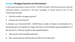
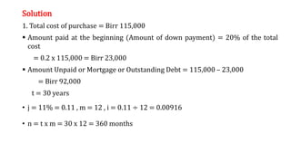
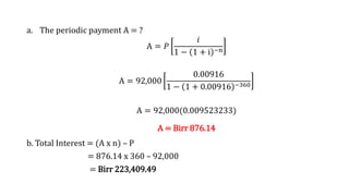
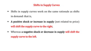
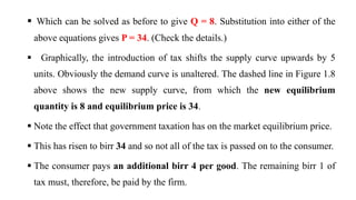
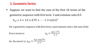
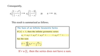
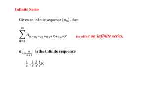
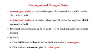
This document provides an overview of the course "Business Mathematics" which covers topics like linear equations, nonlinear equations, and economic applications of linear and quadratic models. The course is targeted at second year ABVM students.
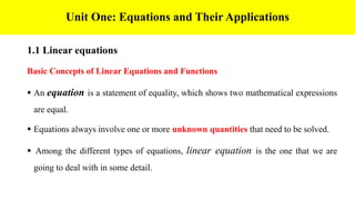
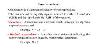
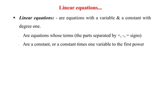
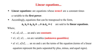
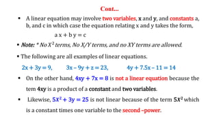
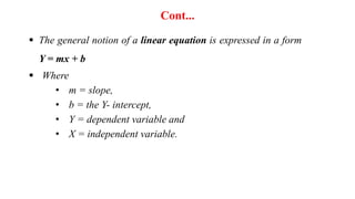
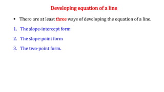
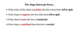
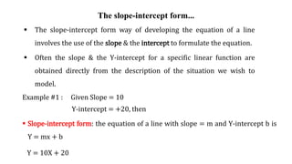
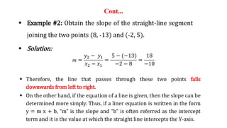
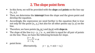
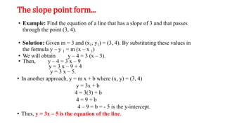
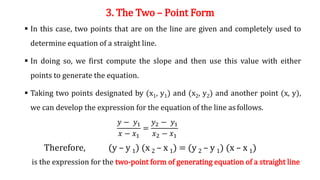
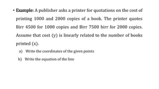
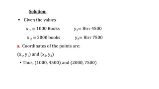
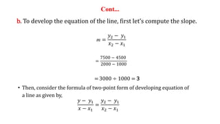
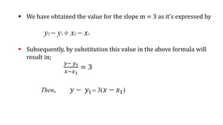
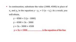
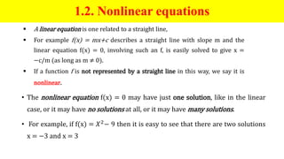
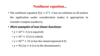
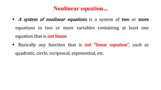
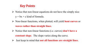
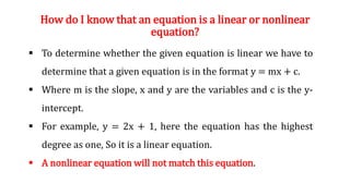
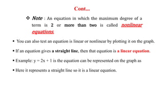
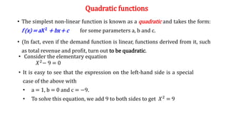
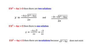
Unit one discusses linear equations, their basic concepts and properties. It also covers developing linear equations using the slope-intercept form, slope-point form, and two-point form. Nonlinear equations are defined as equations with terms of degree two or higher that do not represent straight lines.
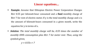
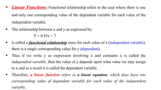
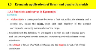
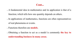
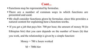
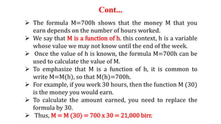
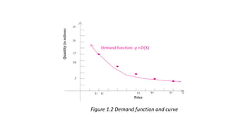
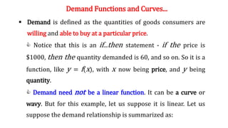
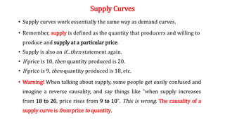
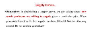
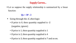
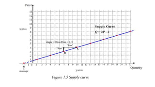
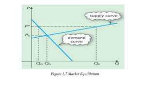
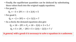
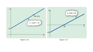
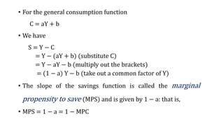
Economic applications of linear and quadratic models are also discussed. Functions and curves are defined in economics, with examples like the relationship between money earned and hours worked given as a simple linear function.


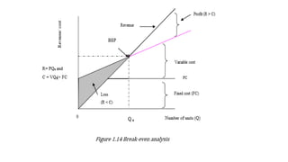
![Break – Even Analysis:
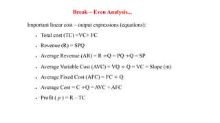
Definition: Breakeven point is the level of sales at which profit is zero.
According to this definition, at breakeven point sales are equal to fixed cost
plus variable cost. This concept is further explained by the following equation:
[Break even sales (BS) = Fixed cost (FC) + variable cost (VC)]
Breakeven sales= Selling price (SP)*Quantity (Q)
VC= VC per unit*Quantity (Q)
SP*Q=FC+ VC/unit*Q
SP*Q-VC/unit*Q=FC
Q(SP/unit-VC/unit)=FC
Q=FC/Sp/unit-Vc/unit- is quantity to be produced or sold at
breakeven point](https://image.slidesharecdn.com/businessmathematicschapter12-240221115832-a716d1bc/85/Business-Mathematics-Chapter-1-2-pptx-89-320.jpg)

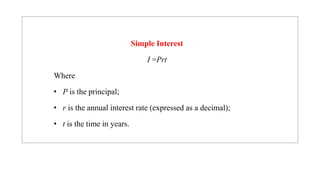
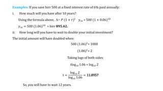
![Future or Maturity Value for Simple Interest
The future or maturity value A of P birr at a simple interest rate r for t years is
A = P (1 +rt).
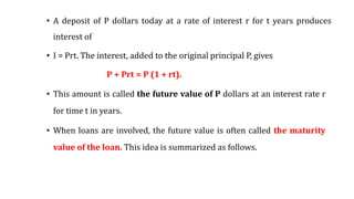
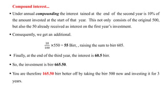
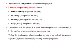
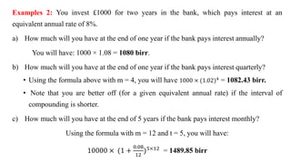
2. Compound Interest: A compound interest system primarily applies to long-term
financial transactions, with a time frame of one year or more.
In this system, interest accrues and compounds upon previously earned interest.
• Compound interest = P × 1 + interest rate)
n−1
]
• Where:
p = principal
n = number of compounding periods](https://image.slidesharecdn.com/businessmathematicschapter12-240221115832-a716d1bc/85/Business-Mathematics-Chapter-1-2-pptx-122-320.jpg)
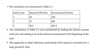
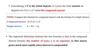
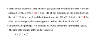
![ In general, to find a formula for compound interest, first suppose that P birr is
deposited at a rate of interest r per year.
The amount on deposit at the end of the first year is found by the simple interest
formula, with t = 1.
A = P (1 + rx1) = P(1 + r)
If the deposit earns compound interest, the interest earned during the second year
is paid on the total amount on deposit at the end of the first year.
Using the formula, A = P(1 + rt) again, with P replaced by P(1 + r) and t = 1, gives
the total amount on deposit at the end of the second year.
A= [P(1 + r)] (1 + r x 1) = P (1 + r)2
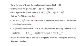
• In the same way, the total amount on deposit at the end of the third year is
A= 𝐏 (𝟏 + 𝐫)𝟑](https://image.slidesharecdn.com/businessmathematicschapter12-240221115832-a716d1bc/85/Business-Mathematics-Chapter-1-2-pptx-130-320.jpg)
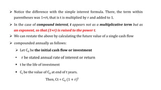
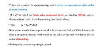
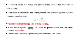
![ Discounting multiple cash flows is simple: we can discount each individual cash
flow and then add the present values (PV).
The general case is present below [the cash flows (C1, C2, C3…Ct) are unequal and
uneven each year]:
ܲݒ0 = (
𝐶1
(1+𝑟)
+
𝐶2
(1+𝑟)2 +
𝐶3
(1+𝑟)3 + ⋯ +
𝐶𝑡
1+𝑟 𝑡)
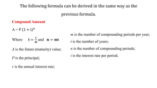
Suppose r is the interest rate, t the number of years, as before, but now suppose
it is compounded m times a year, that is, m is the number of compounding
periods in a year.](https://image.slidesharecdn.com/businessmathematicschapter12-240221115832-a716d1bc/85/Business-Mathematics-Chapter-1-2-pptx-150-320.jpg)