![Control Systems Project: The Smart Bin
Surya Sekhar Chandra
Electrical Engineering
Colorado School of Mines
Golden, CO 80401
Email: schandra@mymail.mines.edu
I. INTRODUCTION
Inactive waste bins result in litter on the floor due to
poor throwing accuracy by humans. A well-designed feedback
controller for an active bin can catch the litter by tracking its
position during its trajectory. The goal of this project is to
design such an active bin with a proper controller that enables
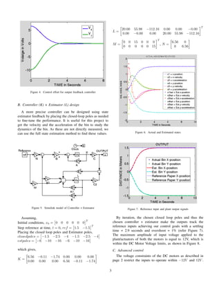
it to catch the litter before it falls to the floor.
II. MODELING
A. Physical Model
Figure 1. Physical model of a bin with four wheels
Figure. 1 shows a physical model of the bin, which consists
of the two DC motors that are attached to the bottom of the
bin. Each of these motors drive a set of wheels that move the
bin in X or Y direction in the room. The bin is attached with
a white patch as it allows the cameras mounted in the room
to accurately detect and locate the 3D position of the bin.
This can be achieved by a simple computer vision detection
algorithm [2]. For this project, a white paper is considered as
litter in general and its 3D location can also be detected using
the same computer vision algorithm.
B. Control Goals
As the main goal of the project is for the bin to actually be
able to catch the paper,the steady state error must be less than
2%, settling time must be less than 3 seconds (assuming high
trajectory) and the overshoot must be below 5% for unit step
reference input.
C. Plant
The plant model consists only of the actuators, which are
the 2 DC motors that drive the bin in X and Y directions.
The inputs to the plant are the voltages (Vx and Vy) applied
to the DC motors and the outputs of the plant are the x and
y locations of the bin.
D. Constraints
The DC motors cannot exceed a maximum power of 5W
and the voltage range that they can be safely operated is from
−12V to 12V .
E. Mathematical Model
Each of the DC motors that forms the plant can be modeled
according to its characteristics as follows:
vi(s)
Vi(s)
=
Kr
(JLs2 + (JR + Lb)s + (bR + K2))
Taking the inverse Laplace transform gives,
¨vi =
Kr
JL
Vi −
(JR + Lb)Kr
JL
˙vi −
(BR + K2
)Kr
JL
vi (1)
The nominal values of the DC motor parameters (taken from
[1]) are considered. Where,
(i) J is the moment of inertia of the rotor = 0.01 kg.m2
(ii) b is the motor viscous friction constant = 0.1 N.m.s
(iii) Ke is the electromotive force constant = 0.01 V/rad/sec
(iv) Kt is the motor torque constant = 0.15 N.m/Amp
(v) R is the electric resistance = 1 Ohm
(vi) L is the electric inductance = 0.5 H
(vii) r is the radius of the wheel = 3 inch = 0.0762 m
(viii) Vi is the voltage applied to the motor that drives in i
axis.
(ix) vi is the linear velocity of the bin in i axis.
(x) i is either X or Y .
This simplifies Equation 1 as
¨vi = 2.286 Vi − 12 ¨vi − 20.02 vi (2)
F. State Space Model
Equation 2 applies to the DC motors in both X-axis and
Y -axis. Since this is a second order system, the state space
representation requires only two states per motor, which
is four states in total. The output required is the x and y
position of the bin and not its linear velocities. Hence, x
and y position of the bin are added to the states of the system.
U =
Vx
Vy
Y =
x
y
X = x vx ˙vx y vy ˙vy
T
1](https://image.slidesharecdn.com/b3163982-672f-45f1-9b47-c17d7705b0fa-151129061251-lva1-app6891/85/Smart-Bin-Advanced-Control-System-Design-Project-1-320.jpg)
![Control Systems Project: The Smart Bin
Surya Sekhar Chandra
Electrical Engineering
Colorado School of Mines
Golden, CO 80401
Email: schandra@mymail.mines.edu
I. INTRODUCTION
Inactive waste bins result in litter on the floor due to
poor throwing accuracy by humans. A well-designed feedback
controller for an active bin can catch the litter by tracking its
position during its trajectory. The goal of this project is to
design such an active bin with a proper controller that enables
it to catch the litter before it falls to the floor.
II. MODELING
A. Physical Model
Figure 1. Physical model of a bin with four wheels
Figure. 1 shows a physical model of the bin, which consists
of the two DC motors that are attached to the bottom of the
bin. Each of these motors drive a set of wheels that move the
bin in X or Y direction in the room. The bin is attached with
a white patch as it allows the cameras mounted in the room
to accurately detect and locate the 3D position of the bin.
This can be achieved by a simple computer vision detection
algorithm [2]. For this project, a white paper is considered as
litter in general and its 3D location can also be detected using
the same computer vision algorithm.
B. Control Goals
As the main goal of the project is for the bin to actually be
able to catch the paper,the steady state error must be less than
2%, settling time must be less than 3 seconds (assuming high
trajectory) and the overshoot must be below 5% for unit step
reference input.
C. Plant
The plant model consists only of the actuators, which are
the 2 DC motors that drive the bin in X and Y directions.
The inputs to the plant are the voltages (Vx and Vy) applied
to the DC motors and the outputs of the plant are the x and
y locations of the bin.
D. Constraints
The DC motors cannot exceed a maximum power of 5W
and the voltage range that they can be safely operated is from
−12V to 12V .
E. Mathematical Model
Each of the DC motors that forms the plant can be modeled
according to its characteristics as follows:
vi(s)
Vi(s)
=
Kr
(JLs2 + (JR + Lb)s + (bR + K2))
Taking the inverse Laplace transform gives,
¨vi =
Kr
JL
Vi −
(JR + Lb)Kr
JL
˙vi −
(BR + K2
)Kr
JL
vi (1)
The nominal values of the DC motor parameters (taken from
[1]) are considered. Where,
(i) J is the moment of inertia of the rotor = 0.01 kg.m2
(ii) b is the motor viscous friction constant = 0.1 N.m.s
(iii) Ke is the electromotive force constant = 0.01 V/rad/sec
(iv) Kt is the motor torque constant = 0.15 N.m/Amp
(v) R is the electric resistance = 1 Ohm
(vi) L is the electric inductance = 0.5 H
(vii) r is the radius of the wheel = 3 inch = 0.0762 m
(viii) Vi is the voltage applied to the motor that drives in i
axis.
(ix) vi is the linear velocity of the bin in i axis.
(x) i is either X or Y .
This simplifies Equation 1 as
¨vi = 2.286 Vi − 12 ¨vi − 20.02 vi (2)
F. State Space Model
Equation 2 applies to the DC motors in both X-axis and
Y -axis. Since this is a second order system, the state space
representation requires only two states per motor, which
is four states in total. The output required is the x and y
position of the bin and not its linear velocities. Hence, x
and y position of the bin are added to the states of the system.
U =
Vx
Vy
Y =
x
y
X = x vx ˙vx y vy ˙vy
T
1](https://image.slidesharecdn.com/b3163982-672f-45f1-9b47-c17d7705b0fa-151129061251-lva1-app6891/75/Smart-Bin-Advanced-Control-System-Design-Project-1-2048.jpg)
![where,
(i) U is the input to the plant.
(ii) X is the state of the system.
(iii) Y is the output of the system.
(iv) x and y are the locations of the bin in X-axis and Y -axis.
(v) Vx and Vy are the voltages applied to the motor that
drives in X-axis and Y -axis respectively.
(vi) vx and vy are the linear velocities of the bin in X-axis
and Y -axis respectively.
The state space representation of the open-loop system
is given by Equation 3
˙X = AX + BU
Y = CX + DU
(3)
A =
0 1 0 0 0 0
0 0 1 0 0 0
0 −20.02 −12 0 0 0
0 0 0 0 1 0
0 0 0 0 0 1
0 0 0 0 −20.02 −12
(4)
B =
0 0
0 0
2.286 0
0 0
0 0
0 2.286
(5)
C =
1 0 0 0 0 0
0 0 0 1 0 0
(6)
These values of matrices A, B and C from Equations 4,5 and
6 will be used throughout the project.
III. ANALYSIS
The plant model is an LTI system. To determine the sta-
bility of the open-loop plant from the state space model, the
eigenvalues of the matrix A are found to be
0, 0, −9.997, −9.997, −2, −2
Out of these six eigenvalues, four are negative and in the
left hand plane. These are the stable poles. The remaining two
are at the origin that make the open-loop plant system unstable.
The Controllability and Observability matrices of the fol-
lowing state space representation can be obtained by using the
Matlabs ctrb and obsv functions. The rank(ctrb(A, B)) = 6,
which is a full row rank. Therefore, the representation is
completely controllable. Similarly, rank(obsv(A, C)) = 6,
which is a full column rank. Therefore, the representation is
completely observable. This is in minimal form. Thus, through
feedback control it is possible to move all the poles to desired
locations.
IV. DESIGN
A. Output Feedback Controller
The position of the bin can be controlled by a negative
output feedback and using the stationary papers position as a
step reference at time, t = 0. A Simulink model of the system
with output feedback is shown in Figure. 2
Figure 2. Simulink model of output feedback controller
Since the motors that control x and y positions are not
coupled in the state space model, they can be controlled by
using a controller of the form K0 = gain ∗
1 0
0 1
(any
other form would mean a coupling between control of x and
y positions of the Bin) and N = K0. By iteration, a gain value
of K0 =
6.5 0
0 6.5
will result in the output (bin position)
tracking the reference (stationary paper position) within our
control goal requirements.
Figure 3. Reference inputs and plant outputs
The settling time = 3 seconds and overshoot = 2% (refer
to Figure. 3) which is within the control limits. Adding the
feedback control made all the eigenvalues of the system
negative and hence asymptotically stable. Voltage input (refer
to Figure. 4) is within the operating limit [1] (|V | <= 12V )
of a DC motor. The output feedback does not allow for a more
precise control, as our output does not consist of all the states.
2](https://image.slidesharecdn.com/b3163982-672f-45f1-9b47-c17d7705b0fa-151129061251-lva1-app6891/85/Smart-Bin-Advanced-Control-System-Design-Project-2-320.jpg)
![Figure 8. Control effort (Input to the plant)
This makes the system behavior non-linear. This model can be
added to the present model in Simulink by using a saturation
block as shown in Figure 9.
Figure 9. Simulink model of controller + estimator with saturation
Simulating this model for a constant step reference of
[1.5 2.5]T
at time = 0 seconds results in a settling time 4.5
seconds.(refer Figure 10). This does not meet our control
goals.
As the reference location gets farther away from the initial
bin location, the bin cannot reach the reference location
within 3 seconds with a magnitude of maximum input voltage
saturated to 12V (refer Figures 10 and 11). This can be
overcome by incorporating a turbocharger into our model. A
turbocharger is a device that releases highly compressed air
at high speeds to momentarily produce a high force, thrusting
forward the object that it is attached to it. It can be used as a
booster which thrusts the bin forward when the bin is lagging
behind and working at its maximum possible input (+12V or
−12V ). In this case, two turbochargers are to be attached to
the bin in both the X and Y directions. The model of the bin
Figure 10. Reference input and plant output signals
Figure 11. Control effort (Input to the plant)
with a turbocharger attached is shown in Figure 12.
The turbocharger can be modeled as a Force,
F = ma (7)
Where,
(i) m is mass = mass of the bin + 2 motors + 4 wheels + 2
turbochargers = 2 kg (approximately)
(ii) a is the acceleration, By using a turbocharger that pro-
duces a Force of around 45 N , produces an acceleration
a = 22.5 m/s2
.
The modified state space representation including the tur-
bocharger is given in Equation 8.
˙X = Ax + Bu + BtT (8)
4](https://image.slidesharecdn.com/b3163982-672f-45f1-9b47-c17d7705b0fa-151129061251-lva1-app6891/85/Smart-Bin-Advanced-Control-System-Design-Project-4-320.jpg)
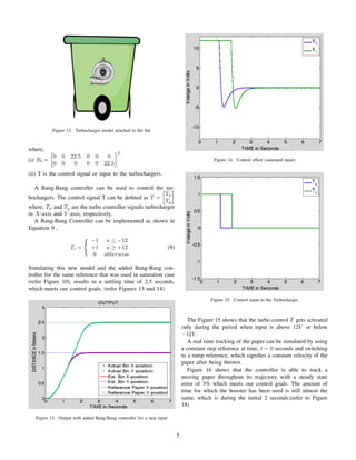
![Figure 16. Output with added Bang-Bang controller for a step and ramp
(mixed) input
Figure 17. Control effort (saturated input)
V. DISCUSSION
The results of the controller design without saturation shows
that the bin starting from rest can track a stationary paper that
is less than 1.5 m away within a settling time of 3 seconds.
Incorporating the non-linearity due to saturation of the input
increases the settling time to above 3 seconds for a stationary
paper that is farther away.It cannot track a moving paper as
the velocity of the bin will not be able to match the paper
velocity without going above 12V of input voltage to the
motors. Adding a turbocharger to the model and controlling it
with a Bang-Bang controller allows the bin to track the model
within the required settling time of 3 seconds for a stationary
paper that is farther than 1.5 m. It also comfortably tracks a
moving paper with low velocities under 0.8 m/s.
Figure 18. Control input to the Turbocharger
VI. CONCLUSIONS AND FUTURE WORK
The advanced controller design used successfully achieves
all the control goals allowing the active bin to catch the
paper. The turbochargers used increase the cost of the bin
significantly, but it gives the much needed thrust for the slow
DC motor driven bin that is trying to catch the paper before it
falls to the floor. Thus, the turbocharger with a Bang-Bang
controller was necessary in addition to the state feedback
controller for achieving the control goals. Future work for
this project would be to explore the options for different
high torque and high speed motors, incorporating which will
increase the range of velocities of the paper the bin can
track.Also, to implement the computer vision algorithm that
detects and locates the bin and the paper by using objection
detection and tracking techniques [2].
REFERENCES
[1] DC Motor Speed: Simulink Controller Design by Matlab Control
Tutorials.
[2] Ta, Duy-Nguyen, et al. Surftrac: Efficient tracking and continuous object
recognition using local feature descriptors. Computer Vision and Pattern
Recognition, 2009. CVPR 2009. IEEE Conference on. IEEE, 2009.
[3] Brogan, William L. Modern control theory. (1991).
6](https://image.slidesharecdn.com/b3163982-672f-45f1-9b47-c17d7705b0fa-151129061251-lva1-app6891/85/Smart-Bin-Advanced-Control-System-Design-Project-6-320.jpg)

This document describes the design of an active waste bin that can track and catch litter using feedback control. The bin is modeled using a physical model and state space equations. An output feedback controller is designed but does not meet precision requirements. A state estimator and controller are designed to precisely control the bin's position. Nonlinearities from motor voltage limits reduce performance. A turbocharger and Bang-Bang controller are added to boost the bin and allow it to track stationary or moving litter within 3 seconds.