This paper presents a design and simulation for a metal cutting machine's position control using static output feedback and full state feedback H2 controllers, employing MATLAB/Simulink. Performance analysis revealed that the full state feedback controller significantly outperforms the static output feedback controller, particularly in reducing overshoot and settling time. The study provides detailed simulations and comparisons indicating improved control for metal cutting processes.

1. 27
Metal Cutting Tool Position Control using Static Output Feedback and Full State Feedback 2H Controllers
Mustefa Jibril1
, Messay Tadese1
, Roman Jirma2
1
Msc, School of Electrical & Computer Engineering, Dire Dawa Institute of Technology, Dire Dawa, Ethiopia
2
Msc, School of Industrial & Mechanical Engineering, Dire Dawa Institute of Technology, Dire Dawa, Ethiopia
mustefa.jibril@ddu.edu.et
Abstract: In this paper, a metal cutting machine position control have been designed and simulated using
Matlab/Simulink Toolbox successfully. The open loop response of the system analysis shows that the system needs
performance improvement. Static output feedback and full state feedback H 2 controllers have been used to increase
the performance of the system. Comparison of the metal cutting machine position using static output feedback and
full state feedback H 2 controllers have been done to track a set point position using step and sine wave input signals
and a promising results have been analyzed.
[Mustefa Jibril, Messay Tadese, Roman Jirma. Metal Cutting Tool Position Control using Static Output
Feedback and Full State Feedback 2H Controllers. Rep Opinion 2020;12(9):27-32]. ISSN 1553-9873 (print);
ISSN 2375-7205 (online). http://www.sciencepub.net/report. 7. doi:10.7537/marsroj120920.07.
Keywords: Metal cutting machine, Static output feedback, Full state feedback H 2 controllers
1. Introduction
A metal cutting machine or cutter tool is any tool
that is used to separate some metallic material from
the work piece by means of cutting. Cutting may be
accomplished by single-point or multipoint tools.
Single point tools are used in turning, shaping, planing
and similar operations, and remove material by means
of one cutting edge. Cutting tool materials must be
harder than the material which is to be cut, and the
tool blade must be in accurate position. The
Coordinate position of the blade might be 1D
(dimension), 2D and 3D and it must be able to
withstand the disturbances that arise for example from
the force generated in the metal-cutting process. Also,
the tool must have a specific geometry, with clearance
angles designed so that the cutting edge can contact
the work piece without the rest of the tool dragging on
the work piece surface.
2. Mathematical Modeling
A solenoid system is fed with an electrical
voltage. The force exerted by the solenoid system is
proportional to the current. This force controls the
hydraulic actuator input. The hydraulic actuator
system is fed with fluid from a constant pressure
source in which the compressibility of the fluid is
negligible. An input displacement x moves the control
valve; thus fluid passes in to the upper part of the
cylinder and the piston is forced to move horizontally.
A low power displacement of x (t) causes a large high
power displacement y (t). The output displacement
moves the cutter blade. The system layout is shown in
Figure 1 below.
Figure 1 Metal Cutter Machine
The solenoid coil circuit equation becomes
   
 
 1
di t
e t Ri t L
dt
 
Taking Laplace transform and arranging the
transfer function between the input voltage and the
output current become
 
 
 
1
2
I s
E s Ls R


The force on the shaft is proportional to the
current i (t) so that
   3iF K i t

2. Report and Opinion 2020;12(9) http://www.sciencepub.net/report ROJ
28
Taking Laplace transform and arranging the
transfer function between the input current and the
output force become
 
 
 4i
F s
K s
I s

The force balance equation of the control valve
becomes
 
2
2
5
d x dx
M B Kx F
dt dt
  
Taking Laplace transform and arranging the
transfer function between the input force and the
output displacement become
 
 
 2
1
6
X s
F s Ms Bs K

 
The flow rate of the fluid Q is related to the input
displacement x (t) and the differential pressure across
the piston will be
   , 7Q g x P
Using Taylor series linearization technique we
have
 
0 0 0 0, ,
8x p
x p x p
g g
Q x P k x k P
x P
    
      
    
Where
   0 0, ,g g x P and x p
is the
operating point, the piston developed a force which is
the area of the piston A multiplied by the pressure P.
The applied force to the mass become
 
2
2
9
d y dy
AP m b
dt dt
 
Where
m mass of the cutter
b Damping coefficient of the piston
Substituting Equation (8) in to Equation (9)
yields:
   
2
2
10x
p
A d y dy
k x Q m b
k dt dt
  
The fluid flow is proportional to the to the piston
movement as
 11qQ K y
Substituting Equation (11) in to Equation (10)
and rearranging yields:
 
2
2
12qx
p p
AKAk d y dy
x m b y
k dt dt k
  
Therefore the transfer function between the
output displacement and input displacement will be:
 
 
 
2
13
x
p
q
p
Ak
kY s
X s AK
ms bs
k
 
  
 
 
   
 
Therefore, the overall transfer function between
the input voltage and the output cutter blade position
can be obtaining by multiplying Equation (2), (4), (6)
and (13).
 
 
     
1
2 2
2
i
Y s K K
G s
E s Ls R Ms Bs K ms bs K
 
    
Where
1
2
x
p
q
p
Ak
K
k
AK
K
k
 
   
 
 
   
 
The metal cutting machine parameters is shown
in Table 1 below
Table 1 Metal cutting machine parameters
No Parameters Symbol Value
1 Resistance R 100 ohm
2 Inductance L 13 H
3 Spring stiffness attached to control valve K 12 N/m
4 Damping coefficient attached to control valve B 3.3 N-s/m
5 Mass of the control valve M 1.4 Kg
6 Force current constant iK 18 N/A
7 Fluid piston constant qK 0.25
1 Mass of the cutter blade m 3 kg
2 Area of the piston A 0.25 m2
3 Damping coefficient of the piston b 6.3 N-s/m
4 Displacement constant xk 8
5 Pressure constant pk 4

3. Report and Opinion 2020;12(9) http://www.sciencepub.net/report ROJ
29
The transfer function of the system then becomes
 
 
  5 4 3 2
54.6 663.4 2725 7818 10630
9
7584s s s s
Y s
G s
E s s



  
The state space representation of the system
becomes
 
12.15 6.239 4.474 3.042 1.085 0.03125
8 0 0 0 0 0
0 4 0 0 0 0
0 0 2 0 0 0
0 0 0 2 0 0
0 0 0 0 0.04121
x x u
y x
       
   
   
    
   
   
   
   


3. The Proposed Controllers Design
3.1 Static Output Feedback Controller Design
Consider a linear time invariant system:
           14x t Ax t Bu t y t Cx t   
Where
   x t x t  
      1
, ,n m
x t R u t R y t R  
are state,
control and output vectors, respectively; A, B, C are
constant matrices of appropriate dimensions.
The feedback control law is considered in the
form
         15u t Fy t FCx t Kx t  
where F is a static output feedback controller
gain matrix. The closed-loop system is then
     16cx t A x t 
where
cA A BFC 
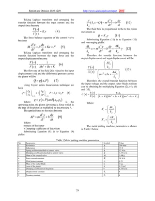
The block diagram of the cutter system with
static output feedback controller gain matrix is shown
in Figure 2 below.
Figure 2 Block diagram of the cutter system with
static output feedback controller gain matrix
It is well known that the fixed order dynamic
output feedback control design problem is a special
case of the static output feedback problem, since the
closed-loop system for the fixed order case has
exactly the same structure as the static case with
appropriately augmented system matrices [5].
Therefore, study of static output feedback problem
includes more general scope of control problems. To
assess the performance quality a quadratic cost
function known from LQ theory is often used.
However, in practice the response rate or overshoot
are often limited. Therefore, we include into the LQR
cost function the additional derivative term for state
variable to open the possibility to damp the
oscillations and limit the response rate.
             
0
17
T T T
cJ x t Qx t u t Ru t x t S x t dt 

   
 
For this system the static output feedback
controller gain matrix becomes
 3.32F 
Then the feedback control law is becoming
         
 
3.32 0 0 0 0 0.1368172
0 0 0 0 0.1368172
u t y t x t
K
 

3.2 Full State Feedback 2H Controller
Design
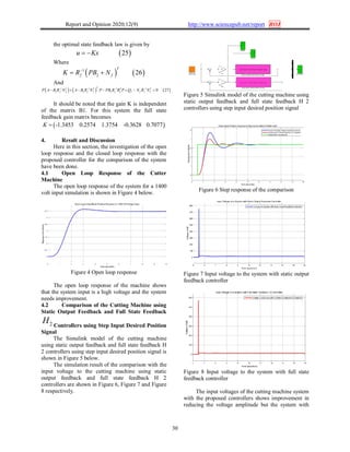
Consider Figure 3 and assume that
 
1 2
1 120 18
0 0
A B B
M C D
I
 
   
  
Figure 3 A full state feedback system.
From Equation (18),
     1 2 19x Ax B d t B u t  
       1 12 20e t C x t D u t 
     21y t x t
Assuming that d (t) is the white noise vector with
unit intensity
        2
2
22T
ed H
T s E e t e t
Where
 1 1 1 12 12 122 23T T T T T T T
e e x C C x x C D u u D D u  
With Equation (19) and Equation (22), the
minimization of
  2
ed H
T s
is equivalent to the
solution of the stochastic regulator problem. Setting
 1 1 1 12 12 12, 24T T T
f f fQ C C N C D and R D D  

4. Report and Opinion 2020;12(9) http://www.sciencepub.net/report ROJ
30
the optimal state feedback law is given by
 25u Kx 
Where
   1
2 26
T
f fK R PB N
 
And
     1 1 1 1
2 2 2 0 27
T
T T T T
f f f f f a f f f fP A B R N A B R N P PB R B P Q N R N   
      
It should be noted that the gain K is independent
of the matrix B1. For this system the full state
feedback gain matrix becomes
 -1.3453 0.2574 1.3754 -0.3628 0.7077K 
4. Result and Discussion
Here in this section, the investigation of the open
loop response and the closed loop response with the
proposed controller for the comparison of the system
have been done.
4.1 Open Loop Response of the Cutter
Machine
The open loop response of the system for a 1400
volt input simulation is shown in Figure 4 below.
Figure 4 Open loop response
The open loop response of the machine shows
that the system input is a high voltage and the system
needs improvement.
4.2 Comparison of the Cutting Machine using
Static Output Feedback and Full State Feedback
2H Controllers using Step Input Desired Position
Signal
The Simulink model of the cutting machine
using static output feedback and full state feedback H
2 controllers using step input desired position signal is
shown in Figure 5 below.
The simulation result of the comparison with the
input voltage to the cutting machine using static
output feedback and full state feedback H 2
controllers are shown in Figure 6, Figure 7 and Figure
8 respectively.
Figure 5 Simulink model of the cutting machine using
static output feedback and full state feedback H 2
controllers using step input desired position signal
Figure 6 Step response of the comparison
Figure 7 Input voltage to the system with static output
feedback controller
Figure 8 Input voltage to the system with full state
feedback controller
The input voltages of the cutting machine system
with the proposed controllers shows improvement in
reducing the voltage amplitude but the system with

5. Report and Opinion 2020;12(9) http://www.sciencepub.net/report ROJ
31
full state feedback H 2 controller shows better
improvement. The data of the rise time, percentage
overshoot, settling time and peak value is shown in
Table 2.
Table 2 Step response data
No Performance Data Full state feedback H2 controller Static output feedback
1 Rise time 1.8 sec 1.8 sec
2 Per. overshoot 17 % 34.2 %
3 Settling time 8 sec 12 sec
4 Peak value 4.1 m 4.7 m
As Table 2 shows that the cutting machine
system with full state feedback H 2 controller
improves the performance of the system by
minimizing the percentage overshoot and settling
time.
4.3 Comparison of the Cutting Machine using
Static Output Feedback and Full State Feedback
2H Controllers using Sine Wave Input Desired
Position Signal
The Simulink model of the cutting machine
using static output feedback and full state feedback H
2 controllers using sine wave input desired position
signal is shown in Figure 9 below.
Figure 9 Simulink model of the cutting machine using
static output feedback and full state feedback H 2
controllers using sine wave input desired position
signal
The simulation result of the comparison with the
input voltage to the cutting machine using static
output feedback and full state feedback H 2
controllers are shown in Figure 10, Figure 11 and
Figure 12 respectively.
Figure 10 Sine wave response of the comparison
Figure 11 Input voltage to the system with static
output feedback controller
Figure 12 Input voltage to the system with full state
feedback controller
The input voltages of the cutting machine system
with the proposed controllers shows improvement in
reducing the voltage amplitude but the system with
full state feedback H 2 controller shows better
improvement.
5. Conclusion
In this paper, the design and position control of a
metal cutting machine have been done using static
output feedback and full state feedback H 2
controllers. The open loop response of the system
analysis shows that for the system cutting position of
3.4m, 1400-volt input is needed which is a high
voltage so the system needs performance
improvement. Comparison of the metal cutting
machine position using static output feedback and full
state feedback H 2 controllers have been done to track
a set point position using step and sine wave input

6. Report and Opinion 2020;12(9) http://www.sciencepub.net/report ROJ
32
signals. Both responses show that the cutting machine
system with full state feedback H 2 controller
improves the performance of the system by
minimizing the percentage overshoot and settling
time.
Reference
1. Ching Yang Lin et al. “Integration of Cutting
Force Control and Chatter Suppression Control
into Automatic Cutting Feed Adjustment System
Design” Journal of Machining Science and
Technology, Vol. 24, Issue 1, 2020.
2. Eric Dimla et al. “Online Metal Cutting Tool
Condition Monitoring: Force and Vibration
Analyses” International Journal of Machine
Tools and Manufacture, Vol. 40, Issue 5, pp.
739-768, 2020.
3. Yuhan Chen et al. “Enhancing the Machining
Performance by Cutting Tool Surface
Modifications: A Focused Review” Journal of
Machining Science and Technology, Vol. 23,
Issue 3, 2019.
4. Jhon O’Hara et al. “Advances in Micro Cutting
Tool Design and Fabrication” International
journal of Extreme Manufacturing, Vol. 1, Issue
3, 2019.
5. Zhenyu Han et al. “Cutting Deflection Control of
the Blade Based on Real Time Feed Rate
Scheduling in Open Modular Architecture CNC
System” International Journal of Advanced
Manufacturing Technology, Vol. 90, Issue 1, pp.
2567-2579, 2017.
6. Mohanad A. et al. “Impacts of Wear and
Geometry Response of the Cutting Tool on
Machinability of Super Austenitic Stainless
Steel” International Journal of Manufacturing
Engineering, Vol. 2016, Article ID 7213148, 9
pages, 2016.
7. Yuan Liu Chen et al. “A Measurement Method
of Cutting Tool Position for Relay Fabrication of
Micro structured Surface” Measurement Science
and Technology, Vol. 25, Issue 6, 2014.
9/24/2020