Modelling Simulation and Control of a Real System

1. Modeling, Simulation, and Control of
a Real System
Robert Throne
Electrical and Computer Engineering
Rose-Hulman Institute of Technology

2. Introduction
• Models of physical systems are widely used
in undergraduate science and engineering
education.
• Students erroneously believe even simple
models are exact.

3. Introduction
• Obtained ECP Model 210a rectilinear mass,
spring, damper systems for use in both
system dynamics and controls systems labs.
• Models for these systems are easy to
develop and students have seen these types
of models in a variety of courses.

4. Introduction
(mass, springs, and encoder)

5. Introduction
(motor, rack and pinion, damper, and spring
connecting to first cart)

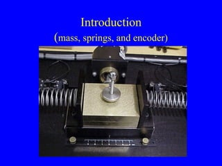
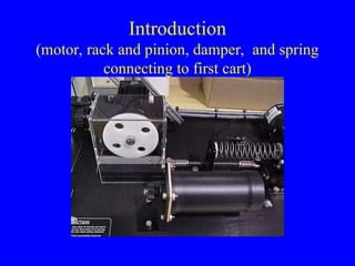
6. Introduction
We developed four groups of labs for the
ECE introductory controls class for a one
degree of freedom system:
• Time domain system identification.
• Frequency domain system identification.
• Closed loop plant gain estimation.
• Controller design based on the model.

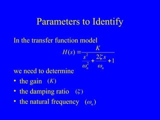
7. Parameters to Identify
In the transfer function model
we need to determine
• the gain
• the damping ratio
• the natural frequency
( )
K
( )

( )
n

2
2
( )
2
1
n n
K
H s
s s

 

 

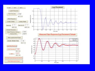
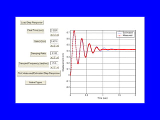
8. Time Domain System Identification
• Log decrement analysis
• Fitting the step response of a second order
system to the measured step response

9. 0 0.2 0.4 0.6 0.8 1 1.2 1.4 1.6 1.8 2
-0.5
0
0.5
1
1.5
Time (sec)
Displacement
(cm)
1
2
3
4
5
6 7
0 0.2 0.4 0.6 0.8 1 1.2
-0.2
-0.1
0
0.1
0.2
0.3
0.4
0.5
0.6
0.7
Time (sec)
Displacement
(cm)
Estimated
Measured

10. 0 0.5 1 1.5 2
-0.2
-0.1
0
0.1
0.2
0.3
0.4
0.5
0.6
0.7
Time (sec)
Displacement
(cm)
Estimated
Measured

11. Frequency Domain System
Identification
• Determine steady state frequency response
by exciting the system at different
frequencies.
• Compare to predicted frequency response.
• Optimize transfer function model to best fit
measured frequency response.

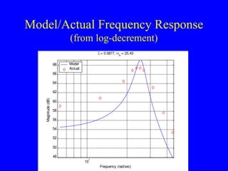
12. Model/Actual Frequency Response
(from log-decrement)
10
1
48
50
52
54
56
58
60
62
64
66
68
Magnitude
(dB)
Frequency (rad/sec)
 = 0.0877, 
n
= 25.43
Model
Actual

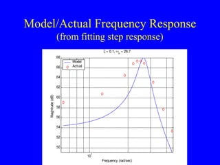
13. Model/Actual Frequency Response
(from fitting step response)
10
1
50
52
54
56
58
60
62
64
66
68
Magnitude
(dB)
Frequency (rad/sec)
 = 0.1, 
n
= 26.7
Model
Actual

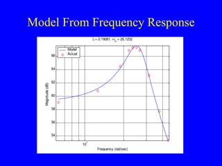
14. Model From Frequency Response
10
1
54
56
58
60
62
64
66
Magnitude
(dB)
Frequency (rad/sec)
 = 0.19081, 
n
= 26.1252
Model
Actual

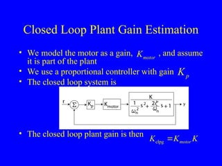
15. Closed Loop Plant Gain Estimation
• We model the motor as a gain, , and assume
it is part of the plant
• We use a proportional controller with gain
• The closed loop system is
• The closed loop plant gain is then
motor
K
p
K
clpg motor
K K K


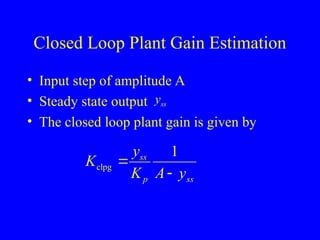
16. Closed Loop Plant Gain Estimation
• Input step of amplitude A
• Steady state output
• The closed loop plant gain is given by
ss
y
clpg
1
ss
p ss
y
K
K A y



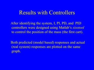
17. Results with Controllers
After identifying the system, I, PI, PD, and PID
controllers were designed using Matlab’s sisotool
to control the position of the mass (the first cart).
Both predicted (model based) responses and actual
(real system) responses are plotted on the same
graph.

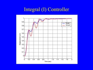
18. Integral (I) Controller
0 0.2 0.4 0.6 0.8 1 1.2 1.4 1.6 1.8 2
0
0.1
0.2
0.3
0.4
0.5
0.6
0.7
0.8
0.9
1
Time (sec)
Displacement
(cm)
Model
Actual

19. ``It doesn’t work!’’

20. Proportional+Derivative (PD)
Controller
0 0.02 0.04 0.06 0.08 0.1 0.12 0.14 0.16 0.18 0.2
0
0.1
0.2
0.3
0.4
0.5
0.6
0.7
0.8
0.9
1
Time (sec)
Displacement
(cm)
Model
Actual

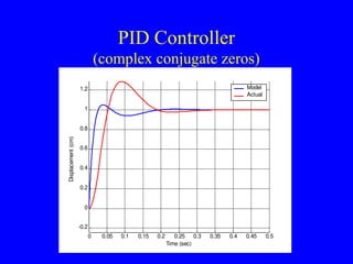
21. PID Controller
(complex conjugate zeros)
0 0.05 0.1 0.15 0.2 0.25 0.3 0.35 0.4 0.45 0.5
-0.2
0
0.2
0.4
0.6
0.8
1
1.2
Time (sec)
Displacement
(cm)
Model
Actual

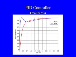
22. PID Controller
(real zeros)
0 0.05 0.1 0.15 0.2 0.25 0.3 0.35 0.4 0.45 0.5
0
0.1
0.2
0.3
0.4
0.5
0.6
0.7
0.8
0.9
Time (sec)
Displacement
(cm)
Model
Actual

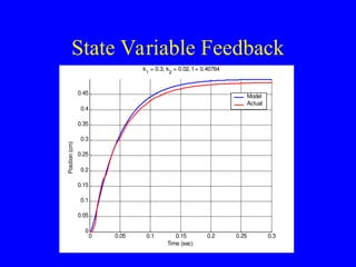
23. State Variable Feedback
0 0.05 0.1 0.15 0.2 0.25 0.3
0
0.05
0.1
0.15
0.2
0.25
0.3
0.35
0.4
0.45
Time (sec)
Position
(cm) k
1
= 0.3, k
2
= 0.02, f = 0.40764
Model
Actual

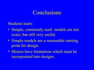
24. Conclusions
Students learn:
• Simple, commonly used models are not
exact, but still very useful.
• Simple models are a reasonable starting
point for design.
• Motors have limitations which must be
incorporated into designs.

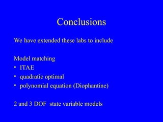
25. Conclusions
We have extended these labs to include
Model matching
• ITAE
• quadratic optimal
• polynomial equation (Diophantine)
2 and 3 DOF state variable models

26. Acknowledgement
This material is based upon work supported
by the National Science Foundation under
Grant No. 0310445