This document describes a contouring control method for CNC machine tools using a linear parameter-varying (LPV) controller. It involves transforming the axis coordinates into a task frame defined by the toolpath direction and velocity. An LPV feedback controller is designed as a function of the toolpath trajectory direction and velocity to minimize estimated contouring error while suppressing vibration. Weighting functions in the controller design are tuned to improve contouring accuracy and bandwidth by adjusting parameters like gains and crossover frequencies.

1. Contouring Control of CNC Machine Tools
Based on
Linear Parameter-Varying Controllers
1

2. CONTENTS
 INTRODUCTION
 THREE AXIS CNC MACHINE
 TRACKING AND CONTOURING ERROR
 CONTOURING ERROR APPROXIMATION
 CONTROLLER OBJECTIVES
 MIMO LPV CONTROLLER DESIGN
1. CONTROLLER STRUCTURE
2. CONTROLLER DESIGN
3. WEIGHTING FUNCTION TUNNING
 CONCLUSION
 REFERENCES
2

3. INTRODUCTION
 CNC or computer-numerical-control machines.
 High speed , high tolerance , precise surface finishing.
 CNC variants : Mills, lathes, EDM, 3d printer, etc.
 Contouring error : deviation of the cutting tool from the toolpath trajectory.
 Servo control : for achieving a satisfactory contouring error.
 tracking control : to minimize the tracking error in each axis individually.
 contouring control cross-coupling control (CCC)
task coordinate frame transformation.
3

4.  CCC method
 Disadvantage : low effectiveness in dealing with nonlinear contours.
 Task coordinate frame transformation
 the axis coordinate system is transformed into tangential-normal-bidirectional
task frame.
 contouring and lag tracking errors : by varying PD and feed-forward
controller.
 Limited to SISO.
4
Real time contour
error calculation
Signal from
compensator
Servo controller in
each axis

5.  The MIMO LPV feedback controller as a function of toolpath trajectory
1. toolpath trajectory direction
2. toolpath trajectory velocity.
 toolpath profiling precision is improved with high feed-rate .
 Controller design approach using
1. advanced gain scheduling control technique based on linear matrix
inequalities.
2. coordinate transformation matrices.
5

6. THREE AXIS CNC MACHINE6
Fig. 1: An illustration of a three-axis CNC machine

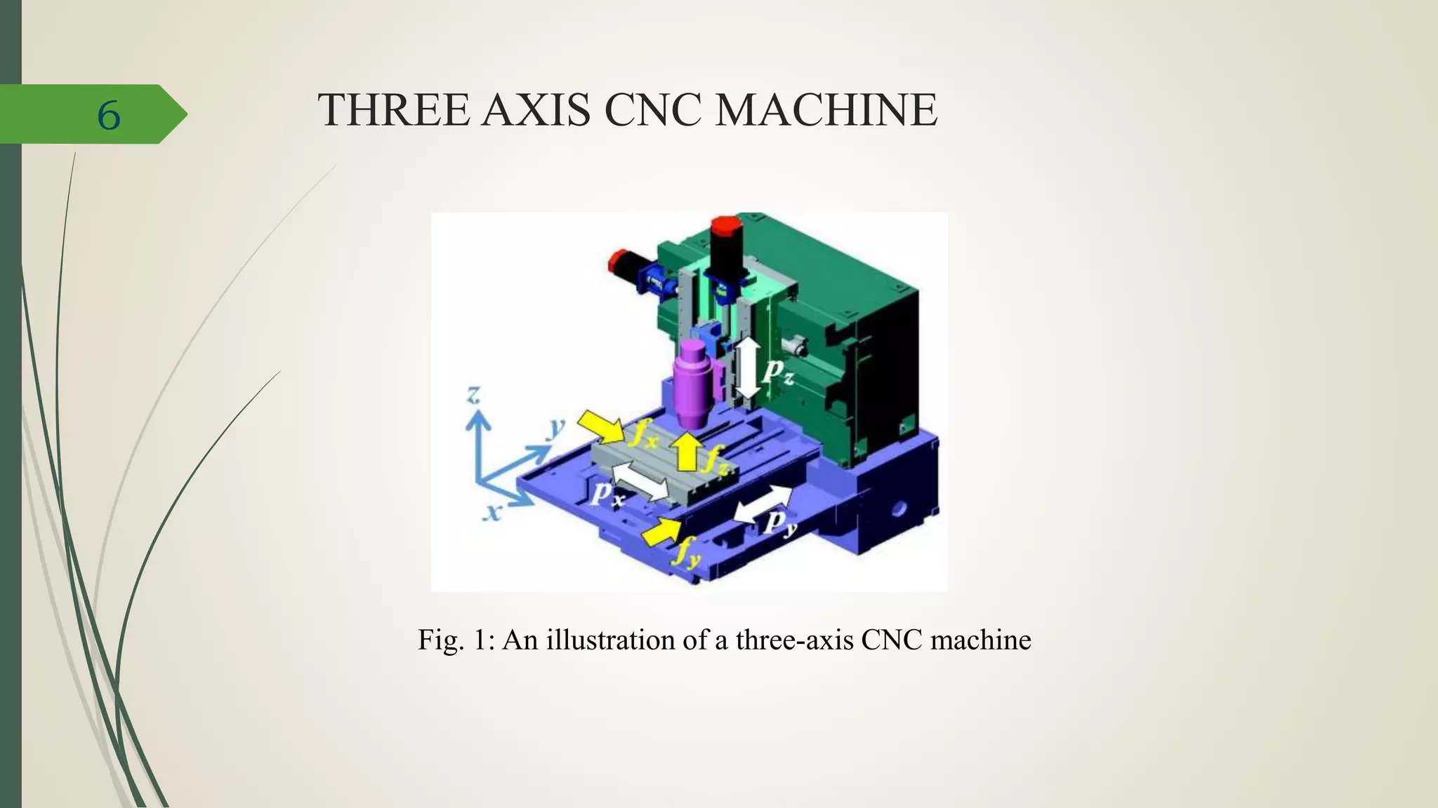
7.  Table with workpiece mass : move in x and y directions.
 Table with machining tool : displaces in z direction.
 Three ball-screw feed-drive systems connected with DC motors for movement.
 Applied voltages current amplifiers DC motors
(𝑣 𝑥, 𝑣 𝑦 and 𝑣𝑧 [V]) (send current commands) (torques generated)
 Torque to the screws : linear displacements (positions) of the tables 𝑝 𝑥, 𝑝 𝑦 and 𝑝 𝑧.
 The positions measurement : linear encoders in real-time for feedback control.
 External forces 𝑓𝑥, 𝑓𝑦 and 𝑓𝑧 [N] : the resultant component of the cutting forces
and friction along the three axes.
7

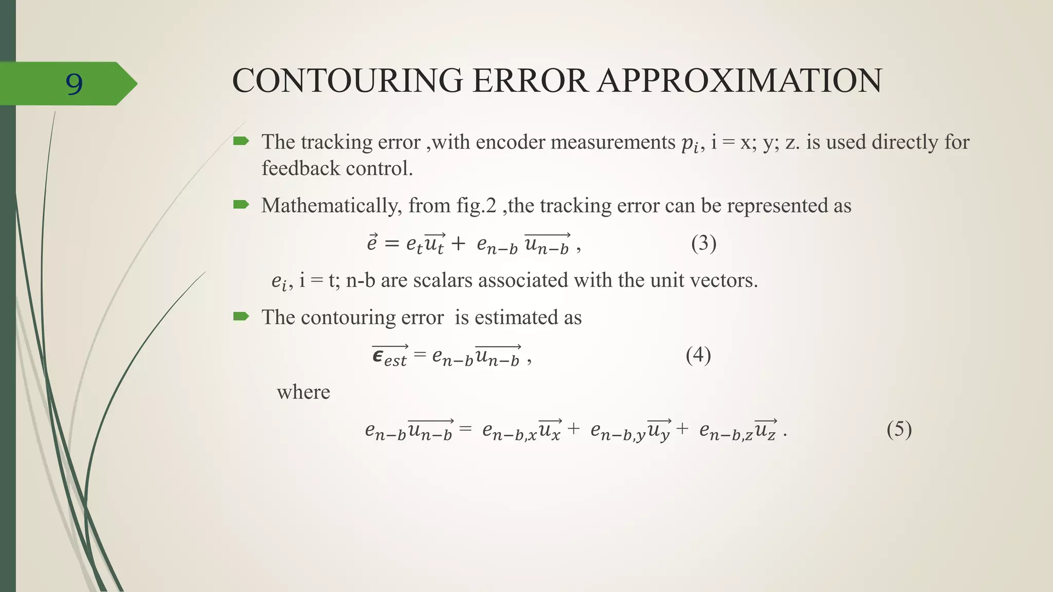
8. TRACKING AND CONTOURING ERROR
 The tracking error : difference between the
table position and its reference in each axis at
each time instant t:
𝑒 𝑡 = 𝑟 𝑡 − 𝑝 𝑡 (1)
 In 3 dimension,
𝑟 𝑡 = [𝑟𝑥(𝑡), 𝑟𝑦(𝑡), 𝑟𝑧(𝑡)] 𝑇
𝑝 𝑡 = [𝑝 𝑥(𝑡), 𝑝 𝑦(𝑡), 𝑝 𝑧(𝑡)] 𝑇 (2)
where 𝑟𝑖, i = x; y; z are the reference signals
in x, y and z directions.
 The contouring error : difference between the
displacement at each time instant and the
shortest-distance point on the reference
trajectory.
Fig. 2: Tracking error and
contouring error in 3axis CNC
machine
8

9. CONTOURING ERROR APPROXIMATION
 The tracking error ,with encoder measurements 𝑝𝑖, i = x; y; z. is used directly for
feedback control.
 Mathematically, from fig.2 ,the tracking error can be represented as
𝑒 = 𝑒𝑡 𝑢 𝑡 + 𝑒 𝑛−𝑏 𝑢 𝑛−𝑏 , (3)
𝑒𝑖, i = t; n-b are scalars associated with the unit vectors.
 The contouring error is estimated as
𝟄 𝑒𝑠𝑡 = 𝑒 𝑛−𝑏 𝑢 𝑛−𝑏 , (4)
where
𝑒 𝑛−𝑏 𝑢 𝑛−𝑏 = 𝑒 𝑛−𝑏,𝑥 𝑢 𝑥 + 𝑒 𝑛−𝑏,𝑦 𝑢 𝑦 + 𝑒 𝑛−𝑏,𝑧 𝑢 𝑧 . (5)
9

10. 10  The relation between measurable vector 𝑒 and unmeasurable scalars (𝑒𝑡; 𝑒 𝑛−𝑏) as
=
𝑇𝑡(α 𝑥, α 𝑦)
𝑇𝑛−𝑏(α 𝑥, α 𝑦)
𝑒, (6)
𝑒 𝑛−𝑏= 𝑒 𝑛−𝑏,𝑥
2
+ 𝑒 𝑛−𝑏,𝑦
2
+ 𝑒 𝑛−𝑏,𝑧
2
(7)
 The transformation matrices 𝑇𝑡 and 𝑇𝑛−𝑏 are given by
𝑇𝑡(α 𝑥, α 𝑦)= 𝑐 α 𝑥 𝑐 α 𝑦 𝑐 α 𝑧
𝑇𝑛−𝑏(α 𝑥, α 𝑦)=
𝑠 α 𝑥
2
−𝑐 α 𝑥 𝑐 α 𝑦 −𝑐 α 𝑥 𝑐 α 𝑧
−𝑐 α 𝑥 𝑐 α 𝑦 𝑠 α 𝑦
2
−𝑐 α 𝑦 𝑐 α 𝑧
−𝑐 α 𝑥 𝑐 α 𝑧 −𝑐 α 𝑦 𝑐 α 𝑧 𝑠 α 𝑧
2
(8)
for an angle, s() and c() denote sin and cos respectively.
𝑒𝑡
𝑒 𝑛−𝑏,𝑥
𝑒 𝑛−𝑏,𝑦
𝑒 𝑛−𝑏,𝑧

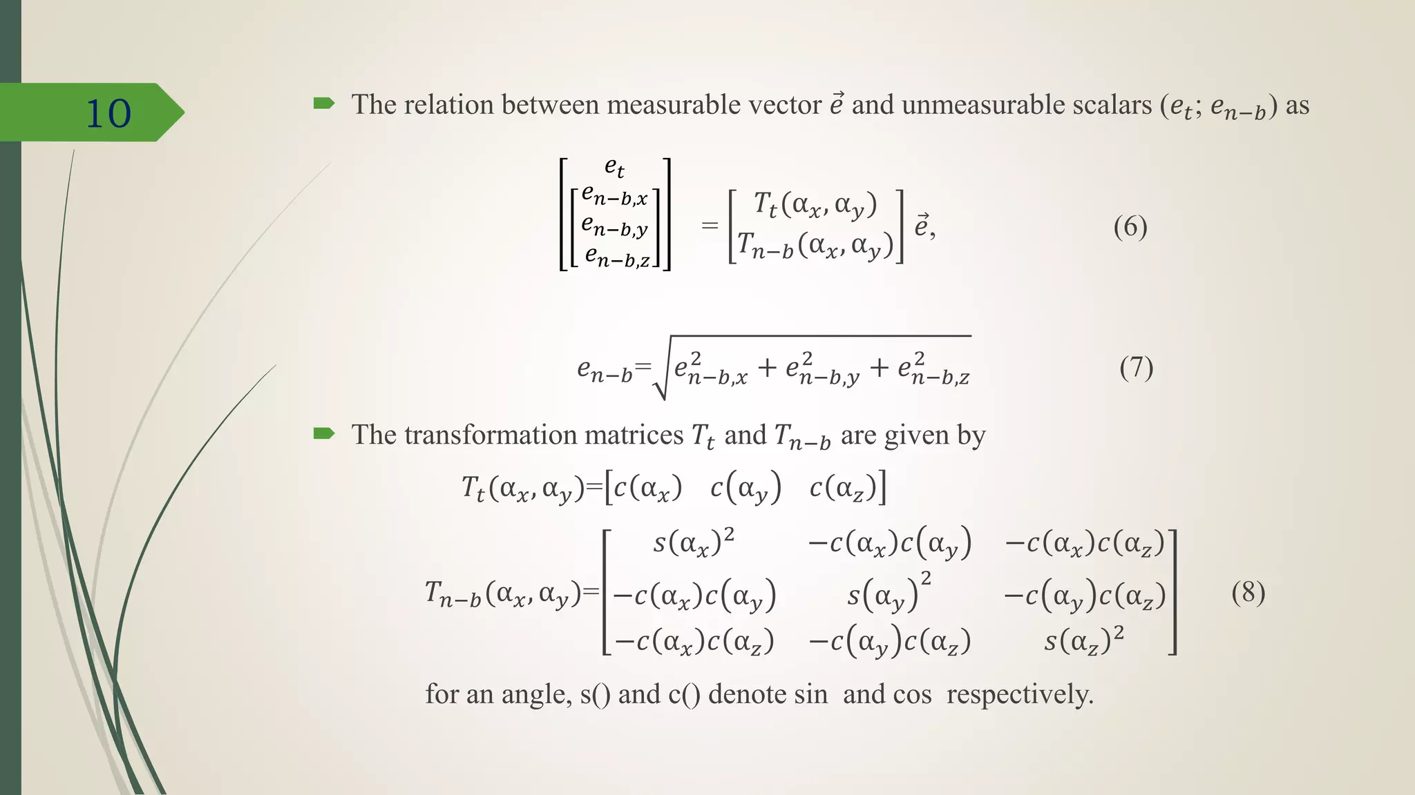
11. CONTROLLER OBJECTIVES
 The mapping from the vector 𝑒 to the scalar 𝑒 𝑛−𝑏 is nonlinear because of (7).
 The mapping from 𝑒 to the vector in the left-hand side of (6) is linear.
 Feedback controllers
 minimizes the approximated contouring error 𝟄 𝑒𝑠𝑡 in (4) and
 also suppresses vibration of the machine due to external forces.
Fig. 3: Feedback structure for contouring error minimization.
where the disturbance force vectors 𝑓 := [𝑓𝑥; 𝑓𝑦 ; 𝑓𝑧] 𝑇,
voltage input vector 𝑣 := [𝑣 𝑥; 𝑣 𝑦; 𝑣𝑧] 𝑇.
11

12. MIMO LPV CONTROLLER DESIGN
 SISO controller : each axis is actuated independently by a feed-drive system.
 A single MIMO controller : function of path direction and velocity.
 compensate for the contouring error and
 to reject the disturbance forces .
 A linear time-invariant (LTI) state-space model of ‘CNC machine’ block in Fig. 3
is expressed by
G:
𝑥 𝑚 𝑡 = 𝐴 𝑚 𝑥 𝑚 𝑡 + 𝐵 𝑚𝑓 𝑓 𝑡 + 𝐵 𝑚𝑓 𝑣 𝑡 ,
𝑝 𝑡 = 𝐶 𝑚 𝑥 𝑚 𝑡
(9)
where 𝑥 𝑚 : state vector,
𝐴 𝑚, 𝐵 𝑚𝑓, 𝐵 𝑚𝑣 and 𝐶 𝑚 : constant system matrices of compatible dimensions.
12

13. 1. CONTROLLER STRUCTURE
Fig. 4: controller structure for contouring control
 The parameter Ɵ(the gain-scheduling parameter) is defined by
Ɵ = [α 𝑥, α 𝑦] 𝑇 (10)
 The first system T(Ɵ) is a parameter-varying matrix which is the coordinate
transformation matrix defined by
T(Ɵ) =
𝑇𝑡(Ɵ)
𝑇𝑛−𝑏(Ɵ)
(11)
13

14.  The output of the system T(Ɵ) are given in the left-hand side of (6) .
 The vector 𝟄 𝑒𝑠𝑡 is given by
𝟄 𝑒𝑠𝑡 = [ 𝑒 𝑛−𝑏,𝑥 , 𝑒 𝑛−𝑏,𝑦 , 𝑒 𝑛−𝑏,𝑧] 𝑇 (12)
 The K(Ɵ; Ɵ) block is a linear parameter-varying (LPV) controller.
14

15. 2. CONTROLLER DESIGN
 For the LTI model G in (9) and the parameter-varying matrix T(Ɵ) in (11), the
design of a gain-scheduling controller K(Ɵ, Ɵ) in Fig. 4 in an LPV form is
𝑥 𝑘
𝑣
=
𝐴 𝑘(Ɵ, Ɵ) 𝐵 𝑘(Ɵ, Ɵ)
𝐶 𝑘(Ɵ, Ɵ) 𝐷 𝑘(Ɵ, Ɵ)
𝑥 𝑘
𝑒𝑡
𝟄 𝑒𝑠𝑡
(13)
where 𝑥 𝐾 is a controller state vector.
 An LPV controller K, function of varying path direction Ɵ and velocity Ɵ.
 Auxiliary signals 𝑧𝑡 ∶ tangential error performance,
𝑧 𝟄 ∶ contouring control performance and
𝑧 𝑣 : control input energy.
15

16.  The signal 𝑓𝑤 : to confine the frequency components of the signal 𝑓 .
 Weighting matrices 𝑊𝑡, 𝑊𝟄, 𝑊𝑉 and 𝑊𝑓 to
 take a tradeoff among these performances,
 improve performance at specific frequency ranges.
Fig. 5: Feedback system for LPV controller design
16

17. WEIGHTING FUNCTION TUNNING
 Parametrizing the weighting functions by
W(s)=
𝑠 𝑀 𝐻
1/𝑘 𝑊 + 𝟂 𝑏
𝑠+ 𝟂 𝑏 𝑀 𝐿
1/𝑘 𝑊
𝑘 𝑊
(14)
where, tuning parameters are
𝑀𝐿 : low frequency gain of 𝑊−1
,
𝑀 𝐻 : high frequency gain of 𝑊−1,
𝟂 𝑏 : unit-gain crossing frequency of 𝑊−1,
𝑘 𝑊 ∶ degree of the function W.
17

18. Weighting function Tuning parameter Effect
𝑊𝟄 Reduce 𝑀𝐿
Increase 𝟂 𝑏
Reduction in contouring
error and to improve the
controller bandwidth.
𝑊𝑡
𝑀𝐿 much larger than that
of 𝑊𝟄
𝟂 𝑏 much smaller than that
of 𝑊𝟄
Reduction in contouring
error and to improve the
controller bandwidth.
𝑊𝑓
Decrease 𝑀 𝐻
Increase 𝑀𝐿
𝟂 𝑏 below the first
principal resonant
frequency.
Improve the vibration
suppression by damping
out resonant modes.
𝑊𝑣 Increase the gain of 𝑊𝑣. Reduction in motor voltage
and to avoid saturation.
18

19. CONCLUSION
 A novel linear parameter-varying (LPV) controller structure.
 The controller consists of two parts,
1. a parameter-varying coordinate transformation matrix which is a function of
machine tool’s reference trajectory angle,
2. a dynamic LPV system which depends on both the trajectory angle and its
velocity.
 The dynamic LPV system was designed by using the well-known advanced gain-
scheduling controller design technique based on linear matrix inequalities.
 Guidelines for tuning weighting functions in contouring controller design.
 Future work : contouring control method to five-axis machine cases.
19

20. REFERENCES
 Masih Hanifzadegan and Ryozo Nagamune, “Contouring Control of CNC
Machine Tools Basedon Linear Parameter-Varying Controllers,” IEEE/ASME
Trans. Mechatronics, vol. 21, pp. 2522–2530, 2016.
 N. Khalick Mohammad, A.E. Uchiyama and S. Sano, “Energy saving in feed
drive systems using sliding-mode-based contouring control with a nonlinear
sliding surface,” IEEE/ASME Trans. Mechatronics, vol. 20, no. 2, pp. 572–579,
2015.
 M. R. Khoshdarregi, S. Tappe, and Y. Altintas, “Integrated five-axis trajectory
shaping and contour error compensation for high-speed CNC machine tools,”
IEEE/ASME Trans. Mechatronics, vol. 19, no. 6, pp. 1859–1871, 2014.
 D. Lam, C. Manzie, and M. C. Good, “Model predictive contouring control for
biaxial systems,” IEEE Trans. Control Systems Technology,vol. 21, no. 2, pp.
552–559, 2013.
20

21. THANK YOU
21