Contents lists available at ScienceDirectBiosensors and Bi.docx

Contents lists available at ScienceDirect
Biosensors and Bioelectronics
journal homepage: www.elsevier.com/locate/bios
Smart Fatigue Phone: Real-time estimation of driver fatigue
using
smartphone-based cortisol detection
Joonchul Shina,b,1, Soocheol Kima,1, Taehee Yoona, Chulmin
Jooa, Hyo-Il Junga,∗
a School of Mechanical Engineering, Yonsei University, Seoul,
South Korea
b Center for Electronic Materials, Korea Institute of Science
and Technology (KIST), Seoul, South Korea
A R T I C L E I N F O
Keywords:
Salivary cortisol
Fatigue
Fluorescence
Smartphone
Electroencephalogram
A B S T R A C T
Numerous studies reported that psychological fatigue is one of
the main reasons leading fatal road crashes. In
order to quantify fatigue level of each subject, we measured a

concentration of salivary cortisol from 4 subjects
(20–40 years of age) using the Smart Fatigue Phone, which
consists of a lateral flow immunosensor and a
smartphone-linked fluorescence signal reader, during 50-min
driving session. Since the salivary cortisol needs to
be measured below 1 ng/mL to distinguish the subjects from
awaken-drivers, we have employed the fluorescence
detection module (Limit of detection: 0.1 ng/mL). To validate
correlation between fatigue status and salivary
cortisol concentration measured by the Smart Fatigue Phone, the
electroencephalogram (EEG) signal was si-
multaneously obtained from the participants. As a result, alpha
wave and concentration of cortisol over time was
highly correlated, reflecting that quantification of salivary
cortisol can be used for real-time monitoring of driver
fatigue (p < 0.05). The Smart Fatigue Phone is expected to be a
useful tool for drivers to recognize their fatigue
status and subsequently to make a decision for driving a car.
Thus, we assume that this fatigue detection system
will consequently minimize road crashes by quantifying salivary
cortisol in real time in the near future.
1. Introduction
Saliva, secreted from the salivary glands, comprises a myriad of
biomolecules related to various disorders, from severe to benign
symptoms, thus applying salivary biomarkers to diagnostic
purposes
(Shin et al., 2018). The interest of saliva-based in-vitro
diagnostics (IVD)
related studies has tremendously increased in recent year with
respect
to several advantages, fulfilling cost-effectiveness and non-
invasive
sampling. Furthermore, the innovative smartphone technologies
are

recently applied to salivary diagnostics as alternatives to blood
for the
point-of-care-testing, which plays a key role in the clinical
fields (Zhu
et al., 2013; Lee et al., 2014; Choi et al., 2014, 2017; Zangheri
et al.,
2015; Shin et al., 2017; Yang et al., 2017; Choi et al., 2019).
The au-
thors have previously developed a noble method to quantify a
degree of
psychological stress with a concentration of salivary cortisol,
which is
also known as a key biomarker for determination of fatigue
status, by
using a smartphone-based colorimetric analysis system (Choi et
al.,
2014, 2017; Yang et al., 2017). Since fatigue has been
considered as one
of the major causes that induces fatal crashes on roadway,
several re-
search teams focused on analyzing data from either electro-
encephalogram (EEG) or driving simulation to study fatigue
patterns of
drivers (Kar et al., 2010; Simon et al., 2011; Li et al., 2012).
Craig et al.
reported that EEG activation increases in theta and alpha
frequency
band and decreases in beta frequency band with respect to time
during
fatigue condition (Craig et al., 2012). In addition, a few studies
showed
the correlation between fatigue condition and concentration of
salivary
fatigue biomarkers, such as cortisol and alpha-amylase (Roberts
et al.,

2004; Yamaguchi et al., 2006). Shin et al. reported that human
salivary
cortisol can be used for an indicator of emotional and fatigue
status
(Shin et al., 2018). The main purpose of this study is to design
the
smartphone-based fluorescence detection system, fulfilling the
high-
sensitivity of a lateral flow immunosensor because less than 1
ng/ml of
salivary cortisol is required to distinguish the subjects in
fatigue con-
dition from awaken-drivers. In addition, previous studies
reported that
low cortisol concentrations were observed in patients, who
suffered
from chronic fatigue syndrome (Cleare, 2004; Roberts et al.,
2004).
Then, the fatigue level assessment of the subjects was
conducted with
electroencephalogram (EEG) measurement to validate our
fatigue de-
tection system. As shown in Fig. 1, we have measured salivary
cortisol
in real time by using the Smart Fatigue Phone, which comprises
a
fluorescence reader, a lateral flow immunosensor, and an
android-
based fluorescence signal application, as well as EEG analysis.
In this
https://doi.org/10.1016/j.bios.2019.04.046
Received 7 February 2019; Received in revised form 11 April
2019; Accepted 23 April 2019
∗ Corresponding author.

E-mail address: [email protected] (H.-I. Jung).
1 The authors contributed equally to this work.
Biosensors and Bioelectronics 136 (2019) 106–111
Available online 24 April 2019
0956-5663/ © 2019 Elsevier B.V. All rights reserved.
T
study, we have enhanced the sensitivity of a lateral flow
immunosensor
for cortisol detection by using fluorescence-based assay (Limit
of de-
tection (LOD): 0.1 ng/mL) instead of application of colorimetric
assay
(LOD: 1.0 ng/mL). In addition, the Smart Fatigue Phone was
designed to
keep drivers away from driving a car in fatigue condition. This
is the
first attempt to determine a degree of fatigue from drivers in
quanti-
tative manner using smartphone-based fatigue detection system
by the
combination of two different modalities (salivary cortisol and
EEG
signal). The fatigue detection system separately consists of a
smart-
phone-based cortisol detection system (Smart Fatigue Phone)
and a
portable EEG measurement device. Based on these results, we
demon-
strated the meaningful study of the smartphone-based cortisol

detection
system for fatigue quantification.
2. Materials and methods
2.1. Methods with subsection as design of experiment
The subjects, who were graduate school students (3 males and 1
female), participated in this study with the following criteria:
age be-
tween 20 and 40 years old (average 29.5 and SD = 1.64),
possession of
a valid driving license, and more than one-year driving
experience. On
the other hand, participants with substance abuse, psychiatric
and sleep
disturbances, or those taking more than 400 mg of caffeine per
day
were excluded. All subjects were tested for 50 min after signing
a
written consent before the experiment. Our study was carried
out under
the human research guidelines of human subjects established by
the
Institutional Review Board (IRB) of Yonsei University, South
Korea.
Experiments were conducted at 1:00 pm when participants
arrived at
the site by providing a driving simulator and a driving
environment
interface, which are 3D-realtime VR software programs, UC-
Win/road,
at Yonsei University. The virtual driving scenario was carried
out on
three large LED monitors (LG Display 27 inches), providing a
130-de-

gree field of view and two side mirrors. The accelerating pedal,
steering
wheel, brake, driver's seat and the body frame of the car were
pur-
chased from Logitech Inc. The entire session of the experiment
con-
sisted of 50 min, including a 5-min practice run and three 15-
min
driving assignments. Thereafter, the saliva samples of each
subject were
then collected at the end of each test (total 4 times). A stand for
holding
a conical tube as a saliva collector was placed in front of each
partici-
pant so that we were able to minimize the influence on the
attention
from subjects. Finally, we measured the concentration of
salivary
cortisol using a smartphone-linked fluorescence detecting
system.
Additionally, cortisol concentration of each subject was
detected using
a commercial ELISA kit (Cambridge, MA, USA) to validate our
mea-
surement system. A standard competitive ELISA method was
applied to
measure optical density values at 530 nm through multiple label
plate
readers (VictorX5, PerkinElmer). The absorbance of plate was
corre-
lated with concentration of cortisol captured in human saliva.
2.2. Design of smartphone-based fluorescence detection system
for
quantification of fatigue

2.2.1. Fabrication of fluorescent lateral flow immunosensor
The antibody vial was diluted to a concentration of 0.25 mg/mL
of
monoclonal cortisol antibody (abCAM, ab1949), which has
negligible
cross-reactivity with cortisone (∼ 0.6%), by the addition of 0.1
M so-
dium bicarbonate (pH 9.3). The diluted solution (1 mL) was
then added
to a Cy3-containing vial (Amersham GE healthcare Inc.) and
was in-
cubated at 23 °C for 2 h with a rotator speed of 120 rpm. The
Cy3
conjugated antibody should be between pH 6.5 and 8.5 by
adjusting the
pH of the compound with HCl (0.1 M). The spin column of the
micro-
centrifuge tube was centrifuged at 1000 g for 30 s to add 250 μL
of the
dye-removing resin. Finally, 250 μL of Cy3 conjugated antibody
was
added to the spin column and centrifuged under the same
conditions.
The intensity of the diluted antibody (9-fold) was measured
with a
fluorescence spectrophotometer (Nanodrop 3300) to determine
the
optimal conditions for the conjugated antibody. The synthesized
com-
pound between high concentration of Cy3 dye and cortisol
antibodies
results in being clogged on the membrane, thus rarely reaching
to the
test line, where cortisol-BSA is immobilized (Fitzerald, USA).

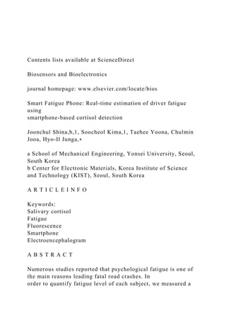
Therefore,
the concentration of each conjugated antibody at 0.001, 0.005,
0.01,
0.02, 0.04, 0.05, 0.08, 0.1, 0.25, 0.5, and 1.0 mg/mL was
applied to the
binding pad, respectively, to evaluate the optimal concentration
of the
synthesized antibody. Finally, the disposable fluorescence based
lateral
flow immunosensor was fabricated with a conjugation pad
(Ahlstrom,
Spain), an absorbance pad (Ahlstrom, Spain), and a
nitrocellulose
membrane (Millipore, USA) which contains a cortisol-BSA and
IgG
antibodies on a test line and control line, respectively, as shown
in Fig.
S1(a). In order to detect fluorescence signal from the test line,
the
collected saliva samples after 2:1 dilution with Phosphate
Buffered
Saline (PBS) were dropped to the strip biosensor for 10 min at
23 °C.
Fig. 1. The experimental procedure for driver fatigue
assessment using the smartphone-based fatigue detection
system. During 50-mins of the experiment, saliva and
EEG signal from the subjects were simultaneously collected and
measured every 15 min, respectively. After collection of both
signals, the correlation between
concentration of salivary cortisol and EEG signal was analyzed.
J. Shin, et al. Biosensors and Bioelectronics 136 (2019) 106–
111
107

2.2.2. Smartphone-based fluorescence reader
The 3D-printed smartphone-based fluorescence reader was
designed
by using CATIA (Dassault Systèmes Inc, Catia V5R14) and a
3D printer
(Measurement Korea Corp., Wiiboox). Dimensions and weight
of the
reader were measured to be 115 mm × 65 mm × 58 mm and 137
g,
respectively. Two green LEDs at 530 nm wavelength (Cree inc.,
XPEBGR-L1-0000-00E03) were employed for the excitation
light
source. The LED light was filtered with optical filters (Chroma
Technology Corp., AT540/25x) to minimize the leakage of LED
light
through the emission filter, and subsequently directed to a strip
bio-
sensor with an incident angle of 45-degree. The fluorescence
emission
from the strip biosensor was then collected by an achromatic
lens
(Thorlabs Inc., AC080-010-A-ML) with a focal length of 10
mm, passed
through the emission filter (Chroma Technology Corp.,
AT605/55m),
and subsequently measured by a two dimensional (2D) charge-
coupled
device (CCD) sensor (HANJIN DATA Corp., 1321191). The
field of view
was determined by 5.7 mm × 3.2 mm (1920 × 1080 pixels) by
ad-
justing the magnification of the fluorescence imaging system at

1x. A
9V battery was employed to supply a stable DC voltage (3.3 V)
to the
LEDs by a voltage regulator (Texas Instruments Inc.,
LM1117IMPX-3.3).
The 2-dimensional fluorescent image was transferred to a
smartphone
(LG Electronics Inc., LG-F400L) using a micro 5-pin connector.
In addition, a strip biosensor (Fig. S1(a)) was loaded into a slot
of
the smartphone-linked fluorescence reader. The customized
application
was designed to capture a fluorescence image and to quantify
the
salivary cortisol concentration. In order to generate the signal
output
from the strip biosensor, the captured image was first converted
to a
grayscale image by computing the average of pixel values over
3 color
channels (i.e. red, green and blue channels) as shown in Fig.
S1(b). The
sensor output was then calculated by evaluating the mean of
pixel va-
lues in the regions of interest (ROI) (IROI) and reference (Iref),
then
subtracting both parameters (IROI - Iref). We evaluated the
difference
between IROI and Iref to compensate for the intensity
fluctuation in the
LEDs and noises arising from the image sensor. The ROI sizes
of the
measurement and reference spot were 3 mm × 1 mm and
0.3 mm × 0.3 mm, respectively. Then, we have decided the
locations

for both regions on the strip biosensor, as depicted in Fig.
S1(c). In
fluorescence measurement experiments, the exposure time was
set to 1/
16 s, which is the smallest coefficient of variation (CV) value
(0.75%).
The detailed description on the noise performance of the reader
is
provided in Fig. 2. The smartphone application, named as the
Smart
Fatigue Phone, based on the android OS was designed for
quantification
of the salivary cortisol. By pressing the capture button, the
embedded
application automatically converted the output signal (IROI-
Iref) into
salivary cortisol concentration using a calibration curve of the
Smart
Fatigue Phone. In addition, a total measurement time was within
7 s,
which includes capturing images, computing cortisol
concentration,
and displaying a driver status on the smartphone.
2.3. EEG measurement
Neurons, neurite cells and blood brain barrier mainly determine
the
electrical activity of the brain. Power spectrum analysis is
usually used
to classify frequencies according to Electroencephalograms
(EEG)
measurement. This analytical method assumes that EEG signal
is a
linear combination of simple oscillations of a particular
frequency and

decomposes each frequency component of the signal to
represent the
amplitude. The EEG is generally divided into θ (theta wave, 3–7
Hz), α
(alpha wave, 8–12 Hz), β (beta wave, 13–29 Hz), and γ (gamma
wave,
30–100 Hz) wave in relation to the range of frequency
(Fitzgibbon
et al., 2004). Theta and alpha are dominant in deep sleep,
emotionally
stable and relaxed states, whereas Beta and gamma waves are
mainly
observed in mental instability and complex problem solving,
respec-
tively. The parietal lobe near the forehead has a somatosensory
cortex
responsible for movement and sensory information, and the
occipital
lobe plays an important role in primary visual processing. The
EEG was
recorded via a 20-channel cognitive wireless EEG system
(Quick-20
system, Cognionics, USA), with the following settings: 1 kHz
sampling
and band pass filtering at 0.05–100 Hz. The silver electrodes
were at-
tached to Fp1, Fp2, F3, F4, F7, F8, C3, C4, T3, T4, P3, P4, T5,
T6, O1,
and O2 according to the international 10–20 method (Okamoto
et al.,
2004). In addition, we set up low pass filtering at 50 Hz,
thereby
sampling EEG data. The following band frequency was analyzed
and
quantified in absolute power for 3 consecutive 15 min of the
driving

test.
3. Result and discussion
3.1. Noise performance of fluorescence reader
We measured noise characteristics of LEDs and image sensor to
figure out the optimal exposure time for highly accurate
detection
system for salivary cortisol concentration. In order to
characterize dark
and readout noise from the Smart Fatigue Phone, numerous
images were
captured as varying detector exposure times. Then, average of
each
pixel value over the entire detection area, where antibodies and
anti-
gens were conjugated, was calculated. As shown in Fig. 2(a), we
cap-
tured 20 images at each condition with measurement of noise
outputs
and standard deviations. The dark noise and readout noise of the
fluorescence detection system were the smallest at the exposure
time of
1/16 s. In addition, we examined the intensity fluctuation of the
LED
light source. The light emitted from the LED was directly
reached to a
photodetector (Thorlabs Inc., PDA36A-EC). Subsequently, the
fluores-
cence intensities were measured for 2.6 s at a sampling rate of
500 Hz.
The power spectrum of the measured intensity fluctuation is
shown in
Fig. 2(b), along with the intensity fluctuation in the inset.
Interestingly,

the smallest value for intensity fluctuation was detected at 16
Hz fre-
quency. Our experimental results for both readout noise and
LED
Fig. 2. (a) Measured dark and readout noise outputs from the
image sensor at different exposure times. The error bars
indicate the standard deviation obtained with
20 measurements. (b) The power spectral density of the
measured LED intensity fluctuation. The inset shows the
measured intensity of the LED light acquired for
∼2.6 s at a sampling rate of 500 Hz. (c) Measured CV values of
the sensor outputs at various exposure times. All of the results
denote that measurement at the
exposure time of 1/16 s would provide fluorescence signal with
the highest precision.
111
108
intensity fluctuation denoted that the measurement with the
highest
precision could be achieved at the exposure time of 1/16 Hz. In
order to
validate these results, we loaded strip biosensor into the
fluorescence
reader, measured variation of intensities from a strip biosensor
under
various exposure times, and evaluate Coefficient Variation (CV)
as
shown in Fig. 2(c). The smallest CV was detected at the
exposure time

of 1/16 s with 0.75%. Based on these results, our study was
performed
at the exposure time of 1/16 s.
3.2. Validation of smartphone-based fluorescence detection
system
compared to ELISA kit
In this study, we were able to identify the fluorescence signals
from
each lateral flow immunosensor where various concentrations of
cor-
tisol antibody (0.001, 0.005, 0.01, 0.02, 0.04, 0.05, 0.08, 0.1,
0.25, 0.5,
and 1.0 mg/mL) were conjugated with Cy3 dye as shown in Fig.
3(a).
The fluorescence intensity in response to each antibody
concentration
showed that the intensity no longer increased by more than 0.25
mg/
mL (Fig. 3(a)). In addition, a smear of Cy3-conjugated
antibodies on the
membrane was appeared around a test line at the highly
concentrated
condition above 0.25 mg/mL in Fig. S2. Due to interatomic
aggregation
among highly concentrated cortisol antibodies, the enlarged
com-
pounds, conjugated with Cy3 dye, are stuck into the membrane.
In the
light of the above, we determined the optimum concentration of
Cy3-
conjugated cortisol antibodies as 0.25 mg/mL. The calibration
curve of
each concentration (0.1, 0.25, 0.5, 1.0, 2.5, and 5.0 ng/mL) of

salivary
cortisol was described with high coefficient of determination
(r2 = 0.9521) in Fig. 3(b). The equation (1), where x denotes the
con-
centration of cortisol and y refers to signal output (fluorescence
in-
tensity), was then applied to the Smart Fatigue Phone to
evaluate the
cortisol concentration from the captured images.
= ÷
−x e 11.9(y 59.727) (1)
Furthermore, the comparison of concentration for salivary
cortisol
from each subject measured by commercial ELISA kit and the
Smart
Fatigue Phone was presented on Fig. 3(c–f). The error rates of
the results
between strip biosensors and ELISA kit were measured within
10%
( ± 4%) as 7.69, 9.45, 12.14, and 10.58% in figure (c), 10.0,
11.67,
10.51, and 11.65% in figure (d), 13.88, 16.31, 18.98, and
24.28% in
figure (e), and 13.58, 13.66, 12.74, 13.86% in figure (f),
respectively.
The significantly high error rates were monitored in a few strips
since
the different amount of cortisol-BSA was immobilized on a test
line of
Fig. 3. Determination of the optimum concentration for Cy3 dye
conjugated cortisol antibodies. (a) The conjugation of multiple
different concentrations from low to
high (0.001, 0.005, 0.01, 0.02, 0.04, 0.05, 0.08, 0.1, 0.25, 0.5,

and 1.0 mg/mL) and Cy3 dye, respectively, were reacted with
cortisol-BSA that is placed on a test line
of the lateral flow immunosensor. (b) The calibration curve of
the strip biosensors at various concentration (0.1, 0.25, 0.5, 1.0,
2.5, and 5.0 ng/mL) are presented
with high coefficient of determination (r2 = 0.9521) by using
the Smart Fatigue Phone. (c–f) The comparison of cortisol
concentration for each subject over time,
obtained from ELISA and the Smart Fatigue Phone, is
described.
111
109
each strip biosensor by using a strip dispenser, thereby resulting
in low
conjugation between Cy3-conjugated antibodies and cortisol-
BSA. On
the other hand, the similar trend of a concentration shift of
cortisol for
every 15 min was observed in both measurement methods. In
addition,
standard deviation (SD), coefficient of variation (CV), and error
rate of
cortisol concentration, measured by ELISA kit and the Smart
Fatigue
phone from 4 different participants, were calculated as shown in
Table
S1.
3.3. Correlation between salivary cortisol concentration and
alpha wave

signal
EEG signals measured during 60 s ( ± 30 s at the measurement
point) were averaged to minimize the error rate for signal noise
caused
by subject movement during saliva collection. As shown in Fig.
4(a–d),
the significant differences were found in alpha and beta wave
for the
subjects. This observation suggested that brain activity (alpha
wave) of
the frontal lobe increased in the fatigue status. This finding is
consistent
with roles of the frontal lobe rule in attention. All of the
subjects had
high alpha and low beta frequency band during the driving
session
(every 15 min). In other words, the low amplitude in beta
frequency
band appeared in the sleep group. The SD and CV of alpha and
beta
frequency power were calculated (Table S2). In addition, each
con-
centration of cortisol of the subjects was measured by two
different
methods: ELISA kit and Smart Fatigue Phone. The proportional
correla-
tion between alpha wave and cortisol concentration with respect
to
driving time was observed in Fig. 5(a–d). The collected data
were
analyzed statistically using ANOVA (analysis of variance) to
investigate
the correlation between alpha wave and cortisol in fatigue state.
The
ANOVA in the alpha frequency bands showed high interaction

between
EEG and salivary cortisol (p < 0.05). The fatigue effect
appeared im-
mediately in that the increase in frontal Fp1, Fp2, F3, F7, O1
and O2
amplitudes was significant in the entire driving session analysis
(p < 0.05). This finding likely reflected the alpha wave and con-
centration of cortisol depending on a degree of fatigue in
response to
driving time. In addition, we were able to determine the fatigue
status
of each participant based on reference values where less than 1
ng/mL
of cortisol and range from 8μV2–12μV2 of EEG signal are
considered as
fatigue state (Cleare, 2004; Roberts et al., 2004; Fitzgibbon et
al.,
2004).
4. Conclusion
In this study, we have successfully developed the smartphone-
based
fluorescence reader for salivary cortisol detection and evaluated
sig-
nificant correlation between cortisol concentration and the EEG
signals
in response to the fatigue condition during performing a driving
si-
mulation. In order to enhance the sensitivity of the sensor, the
fluor-
escence detection system (a smartphone-based reader and a
lateral flow
immunosensor) was applied because the low level of cortisol
(less than
1.0 ng/mL) is generally detected in the fatigue condition.

Furthermore,
we successfully enhanced the sensitivity of lateral flow
immunosensor
until 0.1 ng/mL, which enabled to distinguish the subjects in the
fatigue
condition from the awaken people. Our system possesses
significant
pros compared with ELISA, electrochemical sensor, Raman
spectro-
scopy, and surface plasmon resonance in terms of ease-to-use,
rapid,
and cost-effective methods. On the other hand, we were only
focused on
salivary cortisol level regarding fatigue status in this study;
additional
fatigue-related biomarkers, such as alpha-amylase and lactate,
are
needed to be studied for correlation with cortisol concentration
to en-
hance accuracy of the fatigue detection system. In addition, the
system
has a cumbersome disadvantage of diluting saliva collected
from sub-
jects into buffers (PBS) and dropping the solution into a strip
biosensor.
In order to improve the drawback of the Smart Fatigue Phone,
we are
currently developing an all-in-one strip biosensor that allows
collecting
saliva sample and detecting cortisol concentration
simultaneously.
Thus, we fully expect our system to be a practical tool for
determination
of fatigue status of drivers to avoid fatal crashes on roadway
before
driving a car.

Declaration of interests
All authors declare that we have no known competing financial
interests or personal relationships that could have appeared to
influ-
ence the work reported in this paper.
Fig. 4. (a–d) The comparison of average power spectrum (alpha
and beta wave) of four participants in response to time (0, 15,
30, and 45 min, respectively).
111
110
CRediT authorship contribution statement
Joonchul Shin: Conceptualization, Methodology, Validation,
Formal analysis, Investigation, Resources, Data curation,
Writing -
original draft, Writing - review & editing, Visualization.
Soocheol Kim:
Conceptualization, Software, Validation, Formal analysis, Data
cura-
tion, Writing - original draft, Writing - review & editing,
Visualization.
Taehee Yoon: Validation, Formal analysis, Resources, Data
curation,
Writing - review & editing. Chulmin Joo: Investigation, Writing
- re-
view & editing, Visualization, Supervision, Funding
acquisition. Hyo-

Il Jung: Conceptualization, Methodology, Validation, Formal
analysis,
Writing - review & editing, Visualization, Supervision, Project
admin-
istration, Funding acquisition.
Acknowledgements
This research was supported by the Bio & Medical Technology
Development Program of the NRF funded by the Korean
government,
MSIP (2015M3A9D7067364), the National Research Foundation
of
Korea grant funded by the Korea government (MSIP) (No. NRF-
2018R1A2A2A15019814), and the Technology Innovation
Program (or
Industrial Strategic Technology Development Program)
(20002631)
funded by the Ministry of Trade, Industry & Energy of Korea.
Appendix A. Supplementary data
Supplementary data to this article can be found online at https://
doi.org/10.1016/j.bios.2019.04.046.
References
Choi, S., Kim, S., Yang, J.S., Lee, J.H., Joo, C., Jung, H.I.,
2014. Sens. Bio-Sens. Res. 2,
8–11.
Choi, S., Hwang, Y., Shin, J., Yang, J.S., Jung, H.I., 2017.
Biochip J. 11 (2), 101–107.
Choi, W., Shin, J., Hyun, K.A., Song, J., Jung, H.I., 2019.
Biosens. Bioelectron. 130 (1),

414–419.
Cleare, A., 2004. Trends Endocrinol. Metabol. 15 (2), 55–59.
Craig, A., Tran, Y., Wijesuriya, N., Nguyen, H., 2012.
Psychophysiology 49 (4), 574–582.
Fitzgibbon, S.P., Pope, K.J., Mackenzie, L., Clark, C.R.,
Willoughby, J.O., 2004. Clin.
Neurophysiol. 115, 1802–1809.
Kar, S., Bhagat, M., Routray, A., 2010. Transport. Res. F
Traffic Psychol. Behav. 13 (5),
297–306.
Lee, S., Oncescu, V., Mancuso, M., Mehta, S., Erickson, D.,
2014. Lab Chip 14, 1437–1442.
Li, W., He, Q.C., Fan, X.M., Fei, Z.M., 2012. Neurosci. Lett.
506 (2), 235–239.
Okamoto, M., Dan, H., Sakamoto, K., Takeo, K., Shimizu, K.,
Kohno, S., Oda, I., Isobe, S.,
Suzuki, T., Kohyama, K., Dan, I., 2004. Neuroimage 21, 99–
111.
Roberts, A., Wessely, S., Chalder, T., Papadopoulos, A., Cleare,
A., 2004. Br. J. Psychiatry
184, 136–141.
Shin, J., Choi, S., Yang, J.S., Song, J., Choi, J.S., Jung, H.I.,
2017. Sensor. Actuator. B.
243, 221–225.
Shin, J., Chakravarty, S., Choi, W., Lee, K., Han, D., Hwang,
H., Choi, J., Jung, H.I., 2018.
Analyst 143, 1515–1525.
Simon, M., Schmidt, E., Kincses, W., Fritzsche, M., Bruns, A.,
Aufmuth, C., Bogdan, M.,

Rosenstiel, W., Schrauf, M., 2011. Clin. Neurophysiol. 122 (6),
1168–1178.
Yamaguchi, M., Deguchi, M., Wakasugi, J., Ono, S., Takai, N.,
Higashi, T., Mizuno, Y.,
2006. Biosens. Bioelectron. 21 (7), 1007–1014.
Yang, J.S., Shin, J., Choi, S., Jung, H.I., 2017. Sensor.
Actuator. B. 241, 80–84.
Zangheri, M., Cevenini, L., Anfossi, L., Baggiani, C., Simoni,
P., Nardo, F.D., Roda, A.,
2015. Biosens. Bioelectron. 64, 63–68.
Zhu, H., Isikman, S., Mudanyali, O., Greenbaum, A., Ozcan, A.,
2013. Lap Chip 13, 51–67.
Fig. 5. (a–d) Correlation between alpha power spectrum and
concentration of cortisol in response to time from four different
subjects.
111
111
Transportation Research Part F 13 (2010) 297–306
Contents lists available at ScienceDirect
Transportation Research Part F
j o u r n a l h o m e p a g e : w w w . e l s e v i e r . c o m / l o c
a t e / t r f
EEG signal analysis for the assessment and quantification of

driver’s fatigue
Sibsambhu Kar *, Mayank Bhagat, Aurobinda Routray
Department of Electrical Engineering, Indian Institute of
Technology, Kharagpur, India
a r t i c l e i n f o
Article history:
Received 20 June 2009
Received in revised form 1 June 2010
Accepted 28 June 2010
Keywords:
EEG
Drivers fatigue
Wavelet entropy
Fatigue scale
1369-8478/$ - see front matter � 2010 Elsevier Ltd
doi:10.1016/j.trf.2010.06.006
* Corresponding author. Tel.: +91 9433366158.
E-mail address: [email protected] (S. Ka
a b s t r a c t
Fatigue in human drivers is a serious cause of road accidents.
Hence, it is important to
devise methods to detect and quantify the fatigue. This paper
presents a method based
on a class of entropy measures on the recorded
Electroencephalogram (EEG) signals of
human subjects for relative quantification of fatigue during
driving. These entropy values
have been evaluated in the wavelet domain and have been
validated using standard sub-
jective measures. Five types of entropies i.e. Shannon’s
entropy, Rényi entropy of order 2

and 3, Tsallis wavelet entropy and Generalized Escort-Tsallis
entropy, have been consid-
ered as possible indicators of fatigue. These entropies along
with alpha band relative
energy and (a + b)/d1 relative energy ratio have been used to
develop a method for estima-
tion of unknown fatigue level. Experiments have been designed
to test the subjects under
simulated driving and actual driving. The EEG signals have
been recorded along with sub-
jective assessment of their fatigue levels through standard
questionnaire during these
experiments. The signal analysis steps involve preprocessing,
artifact removal, entropy cal-
culation and validation against the subjective assessment. The
results show definite pat-
terns of these entropies during different stages of fatigue.
� 2010 Elsevier Ltd. All rights reserved.
1. Introduction
Fatigue is a complex state which manifests itself in the form of
lack of alertness and reduced mental or physical perfor-
mance, often accompanied by drowsiness (Lal & Craig, 2001).
In transportation systems, it is a major cause of fatal road acci-
dents. Earlier research has established that fatigue is
responsible for 20–30% of total road fatalities (Lal, Craig,
Boord, Kirkup
& Nguyen, 2003).
The symptoms of fatigue are non-specific: generally it
manifests in the form of drowsiness, tiredness or weakness.
Fatigue leads to severe deterioration in the vigilance level of
the human driver eventually making them commit mistakes.
The detection and quantification of fatigue can help researchers
to build instruments that will help in early assessment of

fatigue level on-board. There has been considerable research to
detect fatigue from several measurements. Most of them
involve:
(i) Subjective measurements based on questionnaires,
(ii) Psychomotor tests based on reaction time and concentration,
(iii) Measurement of ocular parameters like saccadic movement,
Percentage Closure of Eyes (PERCLOS)
(iv) Measurement of physiological variables like
Electroencephalogram (EEG), Electrooculogram (EOG),
Electromyogram
(EMG), Electrocardiogram (ECG)
. All rights reserved.
r).
298 S. Kar et al. / Transportation Research Part F 13 (2010)
297–306
Few authors have also suggested methods based on steering grip
pressure, skin conductance, Blood Volume Pulse (BVP),
etc. (Cai & Lin, 2007; Healey & Picard, 2005).
Subjective tests are based on standardized questionnaires and
helps in self assessment of fatigue. A number of such ques-
tionnaires are reported in literature (Stanford Sleepiness Scale,
Piper Fatigue Scale, Epworth Sleepiness Scale). Psychomotor
tests include performance assessment of the subject based on
some predefined tasks. It has been observed that the reaction
time and error during audio-visual response test of a subject
increase as the fatigue level of the person increases (Caldwell,
Prazinko, & Caldwell, 2003; Milosevic, 1997).

Eye movement and percentage closure of eyes (PERCLOS) are
two important parameters for detecting drowsiness. It has
been observed that eye movement decreases while blink rate
increases as a person enters into the state of fatigue (Lal &
Craig, 2001). Different techniques have been developed for
measurement of eye movement and blink rate using facial image
of the subject (Papadelis et al., 2007; Singh &
Papanikolopoulos, 1999). Many researchers have used
PERCLOS for non-intru-
sive fatigue detection (Dinges, Mallis, Maislin, & Powell, 1998;
Eriksson & Papanikolopoulos, 1997; Ji, Zhu, & Lan, 2004).
A number of studies on ECG have shown a reduction in heart
rate and change in the heart rate variability during fatigue
(Ishbashi et al.,1999; Jeong, Lee, Park, Ko, & Yoon, 2007).
Research on EMG reveals that when a muscle becomes fatigued,
its
stiffness changes, the amplitude of the EMG signal increases,
and the spectrum shifts towards lower frequencies (Knaflitz &
Molinari, 2003; Park & Meek, 1993).
Amongst a number of indicators that can be used for fatigue
detection, EEG is considered to be the most significant and
reliable. EEG is a record of electric potential from the human
scalp, which is a result of excitatory and inhibitory post-syn-
aptic potentials generated by cell bodies and dendrites of
pyramidal neurons (Lal & Craig, 2001). It is closely associated
with
mental and physical activities. For different activities the EEG
recording may be different either in terms of magnitude or in
terms of frequency or both.
Driving involves various functions such as movement,
reasoning, visual and auditory processing, decision making, per-
ception and recognition. It is also influenced by emotion,
anxiety and many other psychological factors (Lal & Craig,

2001). All the physical and mental activities associated with
driving are reflected in EEG signals. This is the reason for con-
sidering this signal as a reliable indicator of fatigue.
Several methods are used in literature to quantify the EEG
signal. These quantifications involve calculation of features like
energy (Jap, Lal, Fischer, & Bekiaris, 2009; Siemionow, Fang,
Calabrese, Sahgal, & Yue, 2004) and entropy (Papadelis et al.,
2006) in different bands of signals and their interactions.
Classical methods to quantify EEG signal (such as Fourier
Trans-
form) is generally based on power spectral analysis. Such type
of analysis assumes that the signal is stationary within the
analysis window. But, EEG signal is highly non-stationary in
nature and is very difficult to find its complete statistical char-
acteristics either in time domain or frequency domain (Shuren &
Zhong, 2004) rendering most of the classical methods inad-
equate for analysis. In recent times, Wavelet Transform has
been used in EEG signal analysis for detecting epilepsy
(Yamaguchi, 2003), brain injury (Al-Nashash et al., 2003), or
micro-arousal in sleep (Glavinovitch, Swamy, & Plotkin,
2005), etc. It provides a multi-resolution time-scale
representation of the signal and is considered as a potential tool
for
study of non-stationary signals. It offers good time resolution at
high frequencies and good frequency resolution at low fre-
quencies (Daubechies, 1990; Mallat, 1999).
The paper presents characterization of the EEG signals in the
wavelet domain using various entropy measures. The EEG
signals are collected from 30 subjects under varying
experimental conditions representing different levels of fatigue.
The fea-
tures are based on basic index which is the property of an
individual band, ratio index which presents the combined
property

of a number of bands, and entropies which is a measure of
information content. Subjective self assessments have been used
to establish the level of fatigue and also as a confirmatory test
for the proposed method.
the paper has been organized as follows:
Section 2 describes the experiment design and data collection.
In Section 3, the methodology of analysis has been de-
scribed. This includes signal preprocessing, artifact removal,
calculation of entropy and development of a scale for an un-
known fatigue level. Section 4 describes the results along with
discussions.
2. Experiment design
Different sets of experiments were conducted using a 32-
channel Polysomnograph machine to collect EEG data from var-
ious subjects in actual and simulated driving scenario. The EEG
signals were recorded in the laboratory as well as on the test
sites at suitable instants during the experiments. The following
paragraphs depict our experiments and collection of data.
2.1. Subjects and experiment design
The entire set of experiments has been divided into three
categories.
2.1.1. Experiment 1: actual driving and driving related
psychomotor vigilance tests
Experiment 1 was conducted on 21 healthy male participants
(professional drivers) between ages 25 and 35. They were
asked to drive for 1 h in a busy traffic followed by a
computerized subjective test. Then a set of psychomotor tests
i.e.
Complex Reaction Time Test, Action Judgment Test, Speed

Distance Judgment Test, Glare and Vision test were conducted
S. Kar et al. / Transportation Research Part F 13 (2010) 297–
306 299
(Chakraborty, 1998). All the test set-ups were designed to
simulate different types of actual driving activities and are used
to
evaluate the driver’s skill and performance. The EEG data
collected before the commencement of the entire process of
exper-
iment was labeled as ‘Level 1’. On the other hand the EEG data
recorded at the conclusion of the entire procedure was labeled
as ‘Level 2’. All these tests were conducted at specialized
laboratory facilities located at Central Road Research Institute
(CRRI), New Delhi, India.
2.1.2. Experiment 2: simulated driving tasks with sleep
deprivation
Twelve healthy male subjects have been chosen in the age group
of 20–35 years for this experiment. All the subjects were
reported to have no disorders related to sleep. They were asked
to refrain from any type of medicine and stimulus like alco-
hol, tea or coffee during the experiment.
The entire experiment was divided into a number of identical
stages. Each stage started with condition monitoring of each
subject by a medical practitioner. After the subject was declared
fit, he was asked to perform some predefined tasks. These
were: physical exercise on a tread mill for 2–5 min to generate
physical fatigue; simulated driving for about 30 min to gen-
erate physical, visual, and mental fatigue; auditory and visual
tasks for 15 min to generate mental and visual fatigue; finally
the computerized game related to driving for about 20 min. A

single stage of experiment lasted for about 3 h. The experiment
was continued for about 36 h.
Three minute EEG data were recorded at the beginning of the
experiment and at the final phase of each stage when the
subjects were playing the computer game.
2.1.3. Experiment 3: actual driving tests for validation
Seven healthy male subjects (professional drivers) have been
chosen for validating the estimation method under actual
driving condition. The details are given in Table 1 (Section
4.3).
2.2. Acquisition of EEG data
Driving is a complex task involving simultaneous activities of
different parts of the brain. Different lobes of the brain are
related to various functionalities. The frontal lobe is associated
with planning, reasoning, movement, emotion and problem
solving. The parietal lobe is associated with movement,
recognition, perception of stimuli whereas temporal lobe is
associ-
ated with recognition and perception of auditory stimuli,
memory, and speech. This makes the spatial placement of elec-
trodes in EEG recordings a critical parameter. Using the
International 10–20 electrodes placement system, the number of
EEG channels used can be as high as 19 (Lal et al., 2003) or as
low as 4 (Schier, 2000).
In this work, thirteen scalp electrodes were used in addition to
reference and ground to collect the signals from locations
Fp1, Fp2, F3, F4, T3, T4, C3, C4, P3, P4, O1, O2, and CZ
following the international 10–20 system. The sampling
frequency was
kept at 256 Hz with 16 bit A/D conversion.

The experiment was performed in compliance with the relevant
laws and institutional guidelines. The subjects were
asked to file written consents prior to the experiment.
2.3. Collection of subjective data
During the above experiments the drivers were requested to give
subjective feedback, the methodology of which has been
explained in Section 3.5. This feedback is instrumental in
establishing the correlation between the feature-based analysis
and
actual subjective fatigue, and developing a scale for estimating
the unknown fatigue level.
3. Methodology
The method of data analysis involves preprocessing, artifact
removal, and computation of features based on Discrete
Wavelet Transform for estimation of fatigue. The preprocessing
stage includes filtering and normalization followed by arti-
fact removal using wavelet based thresholding.
3.1. Preprocessing
The raw EEG data is contaminated with numerous high
frequency and low frequency noise known as artifacts. The high
frequency noise is due to atmospheric thermal noise and power
frequency noise. The low frequency noise is mainly due to
eye movements, respiration and heart beats. They are
characterized by amplitude in the millivolt range (whereas the
actual
EEG is in microvolt range) in the frequency band of 0–16 Hz
(Krishnaveni, Jayaraman, Aravind, Hariharasudhan, &
Ramadoss,
2006). The raw EEG containing this noise at both ends of the
spectrum was first processed using a band pass filter with cutoff

frequencies of 0.5 Hz and 30 Hz followed by normalization.
Normalization ensures removal of any unwanted biases that may
have crept into experimental recordings. The in-band artifacts
were then removed using a wavelet based technique as will be
explained in the subsequent paragraphs.
297–306
3.2. Artifact removal using discrete Wavelet Transform
Wavelet Transform is a useful tool for time frequency analysis
of neurophysiological signals. Wavelets are small wave like
oscillating functions that are localized in time and frequency
(Daubechies, 1990; Mallat, 1999).
In discrete domain, any finite energy time domain signal can be
decomposed and expressed in terms of scaled and shifted
versions of a mother wavelet w(t) and a corresponding scaling
function /(t). The scaled and shifted version of the mother
wavelet is mathematically represented as
wj;kðtÞ¼ 2
j=2wð2j t � kÞ; j; k 2 Z ð1Þ
A signal S(t) can be expressed mathematically in terms of the
above wavelets at level j as
SðtÞ¼
X
k
sjðkÞ/j;kðtÞþ
X
k

djðkÞwj;kðtÞ ð2Þ
where sj(k) and dj(k) are the approximate and detailed
coefficients at level j. These coefficients are computed using
filter bank
approach as proposed by Rioul and Vetterli (1991).
The original signal S(t) is first passed through a pair of high
pass and low pass filters. The low frequency component
approximates the signal while the high frequency components
represent residuals between original and approximate signal.
At successive levels the approximate component is further
decomposed. After each stage of filtering, the output time series
is
down-sampled by two and then fed to next level of input.
The features extracted from the wavelet decomposition depend
primarily on the type of mother wavelet chosen. It is
known that the best results are obtained when there is a close
resemblance between the signal and the mother wavelet.
The Daubechies family of wavelets has a compact support with
relatively more number of vanishing moments (Mallat,
1999). This makes it a suitable candidate for signal compression
and characterization. By repeated simulation and test we
found that the dB4 (Daubechies family) is most suitable for the
EEG signals in our case.
In this work, the signal has been decomposed into four levels in
which the detail component at level-1 approximately
represents beta (b) band (15–30 Hz), detail component at level-
2 represents alpha (a) band (8–15 Hz), detail component
at level-3 represents theta (h) band (4–8 Hz) whereas the detail
component at level-4 (d2:2–4 Hz) along with approximate
(d1:0.5–2 Hz) component represent the delta (d) band (0.5–4
Hz) of the EEG signal.
As the wavelet coefficients represent the correlation of signal

with the mother wavelet, the signal will generate high
amplitude coefficients at places where artifacts are present.
These coefficients can be eliminated using a simple
thresholding
technique. The threshold can be computed as:
T j ¼ meanðCjÞþ 2 � stdðCjÞ ð3Þ
Here Cj is the wavelet coefficient at jth level of decomposition.
If the value of any coefficient is greater than the threshold
it is reduced to half (Kumar, Arumuganathan, Sivakumar, &
Vimal, 2008). This generates a new set of wavelet coefficients
for
signal without artifacts.
The EEG based parameters have been computed with an 8 s
window with 50% overlapping between successive windows.
3.3. Wavelet relative energy and ratios
The energy at a particular level of decomposition j, which may
correspond to any of the wave group, i.e. d, h, a, b can be
expressed as
Ej ¼
XL
k¼1
½CjðkÞ�
2 ð4Þ
where Cj(k) is the wavelet coefficient (approximate or detailed).
L is the total number wavelet coefficients at the jth level.
Hence the relative energy of a particular band represented by
the resolution level j is given by
pj ¼
EjP
j
Ej

ð5Þ
These relative energy parameters form the basic energy indices
can be used as features for the classification of fatigue.
However many a times it has been observed that these indices
do not show a substantial change under mild fatigue. There-
fore ratio indices are proposed to enhance the contrast among
different levels of fatigue (Eoh, Chung, & Kim, 2005). These
ratio indices include ratios of relative energies of various wave
groups.
In this paper we also propose four different entropic measures
i.e. Shannon, Renyi, Tsallis and Generalized Escort-Tsallis
Entropy as the features to improve the classification in the
presence of uncertainties associated with these energy
bands.
306 301
3.4. Wavelet entropy
Entropy serves as a measure of information (Blanco, Figliola,
Qiuroga, Rosso, & Serrano, 1998; Glavinovitch et al., 2005).
The Shannon’s entropy (SE) is a disorder quantifier (Shannon,
1948) and is a measure of flatness of energy spectrum in the
wavelet domain. It is defined as
SE ¼�
X
j
pj � logðpjÞ ð6Þ
The significance of this entropy can be best understood in terms
of probabilistic concept. A signal having very high energy

content in a particular wave group of EEG accentuates the fact
that it is predominantly composed of particular frequency
band. The concentration of energy in a particular frequency
band indicates lack of randomness in terms of frequency of that
particular signal. Hence the entropy value will be lower for such
signals. On the other hand uniform distributions of energy in
all the wave groups indicate the presence of randomness
associated with the signal resulting in higher entropy value.
Another statistical measure closely related to SE is Rényi
entropy (RE) (Renyi, 1961). The basic definition of RE is given
by
RE ¼
1
1 � q
log
X
j
pqj
" #
ð7Þ
where pj is the relative energy as described earlier and q 2 R is
known as the entropic index. The parameter q confers gen-
erality to this information measure. In the present study we have
used q = 2 and 3 to calculate 2nd and 3rd order entropy.
Both SE and RE are extensive property of a system (Tong,
Bezerianos, Paul, Zhu, & Thakor, 2002). Earlier studies have
shown that SE and RE work well on signal exhibiting short
range interaction (Bezerianos, Tong, & Thakor, 2003; Renyi,
1961; Tong et al., 2002; Torres & Gamero, 2000).

Further search for disorder quantifiers brings out non-extensive
entropies like Tsallis wavelet entropy (TsE) (Tsallis, 1988)
and Generalized eScort-Tsallis entropy (GenTsE) (Poja,
Hornero, Abasolo, Fernandez, & Escudero, 2007). The major
point of
disparity between extensive and non-extensive entropy lies in
the proficiency of the latter in dealing with signals exhibiting
long range interactions. TsE is a non-logarithmic parameterized
entropy defined by Tong et al. (2002) as
TsE ¼
1
q � 1
X
j
½pj � p
q
j � ð8Þ
where q 2 R is an embodiment of degree of non-extensivity. The
variable parameter q, confers the control of modifying the
entropy in concordance with the nature of the signal. Low
values of q work well with signals having long range
interaction,
whereas high q are used with signals plagued with spikes and
sudden abrupt changes. In this study we have used q = 2 for
TsE.
GenTsE (Poja et al., 2007) is defined as
GenTsE ¼
1
q � 1
1 �

X
j
p1=qj
!�q" #
ð9Þ
Where q is the entropy parameter similar to that of TsE. It
shares its non-extensive properties with TsE but differs in its
treat-
ment of probability distributions. The probability distribution is
modified to generate an escort distribution of order q. Such
modifications in probability distributions help one to reveal
information that was interred in the original distribution. The q
value for this study was taken to be 2.
3.5. Subjective assessment
The subjective assessment of fatigue is based on questionnaire.
A set of questions has been selected from standard sleep-
iness scales (Stanford Sleepiness Scale, Piper Fatigue Scale,
Epworth Sleepiness Scale) for the purpose (Appendix A). The
questions were asked through an interactive session. Subject’s
self assessment has been used for final fatigue level assess-
ment on a scale 1–10 with 10 being most fatigued.
3.6. Fatigue scale: estimation of fatigue level
The above parameters have been computed from the EEG
records of the subjects at different levels of fatigue based on a
subjective assessment, as specified in Section 3.5. This helped
to find a method for scaling and estimating unknown fatigue
level from the EEG records. The following procedure is
followed to establish the proposed entropy measures as the
indicator
of fatigue:

Step 1: Selection of important EEG parameters those are most
coherent with the self assessed fatigue at different levels.
Step 2: For every subject, plot each parameter value with
respect to self-estimated fatigue levels and fit a polynomial.
Step 3: Estimate the unknown fatigue level from each of the
above curves.
297–306
Step 4: Compute the mean and variance of the estimated values.
Step 5: Eliminate those estimations which cross a predefined
threshold value. Find the mean estimation of all other
measurements.
4. Results and discussions
4.1. Energy-based analysis
The relative wavelet energy for the a band was calculated
directly from the discrete wavelet coefficients as explained in
Section 3.3. Fig. 1 shows the relative wavelet energy of the a
band of two subjects; one from each type of experiment, for
different stages of fatigue. It has been observed that the a
energy increases with the level of fatigue.
It has already been discussed that sometime the basic energy
indices do not show a substantial change under mild fati-
gued condition and suitable ratio parameters may be better in
differentiating such fatigue levels. In this study we observed
increase in the value of a relative wavelet energy and b relative
wavelet energy and a dip in energy in the low frequency d
band for most of the subjects. This observation led to the choice
of ratio index (a + b)/d1 in this study. The values of this ratio

parameter at different fatigue levels are shown in Fig. 1. We
have observed such variation in most of the subjects from all
types of experiments.
The physical interpretation of these observed variables can be
best understood in terms of energy spectrum. In normal
state the driver’s energy spectrum is primarily composed of low
frequency d waves. At the onset of fatigue the spectral en-
ergy shifts from low frequency bands to high frequency a and b
bands. This observation led to the choice of a ratio index
(a + b)/d1 which amplifies the increase in relative wavelet
energies in high frequency bands and simultaneous decrease in
relative wavelet energy in low frequency bands.
Fig. 1 also show the correspondence between energy based
parameters and subjective assessment at successive stages.
Such observation has also been observed in other experimental
results.
4.2. Entropy analysis
Entropy analysis helps us to capture the essence of spectral
energy distribution changes in a broader perspective. It has
been observed from the energy and ratio analysis that, the
fatigue manifests itself as change in energies in different fre-
quency bands. Wavelet entropies take into account these
relative energies (probabilities) of different frequency bands
and hence project out as single valued quantifiers for study of
changes in energy distribution.
The entropy analysis of two subjects is shown in Fig. 2. An
increasing trend has been observed in entropy values with
fatigue at successive stages. A closer look at the graph
elucidates that the extensive entropies (SE and RE) have better
per-
formance than the non-extensive ones in classifying the fatigue

stages.
Fig. 1. Variation of a band relative energy, ratio (a + b)/d1 and
subjective assessment of two subjects at various levels of
fatigue.
Fig. 2. Variation of different types of entropies of two subjects
at various levels of fatigue.
306 303
A stage wise analysis of the entropy values brings out the
physical significance of this feature. As mentioned in energy
and
ratio analysis, the first stage EEG signal is basically composed
of low frequency d waves. Hence the entire energy distribution
is skewed towards the lower frequencies. This represents a
signal with lower disorder. Therefore, entropy values are lowest
in case of first stage for all the entropies. As the fatigue level
increases the energy in the a and b bands starts to increase. This
leads to the flattening of the energy spectrum. Flattening of
energy distribution means greater disorder, this leads to higher
entropy values at later stages.
Among the above mentioned parameters relative a band energy
is an already established indicator of fatigue (Lal & Craig,
2001; Rosso et al., 2001; Schier, 2000) and the others have been
proposed from the above experimental analysis. It has been
mentioned in the literature that a band relative energy increases
as the fatigue level of a person increases. This has been
observed in both actual (Experiment 1) as well as simulated
(Experiment 2) driving experiments. For Experiment 1, the dif-
ference in fatigue level is less and a band relative energy failed
to indicate that in four subjects (Subject numbers 3, 4, 8, 9).
Whereas the ratio (a + b)/d1 failed in three subjects (Subject

numbers 3, 4, 8) and the entropy parameters failed in only one
subject (subject 4). The result of all the subjects from
Experiment 1 has been shown in Appendix B. Thus proposed
fatigue
indicating parameters may be useful for the detection of fatigue
in human subjects.
4.3. Estimation of fatigue level
A number of parameters have been identified in the previous
sections which show a regular variation with increasing lev-
els of fatigue. These parameters may be combined together to
prepare a scale for the measurement of an unknown fatigue
Table 1
Comparison of estimated fatigue with self-estimation.
Subjects State of the subject Fatigue level
Estimation using proposed EEG
based parameters
Subjective estimation based
on questionnaire
1 Before driving 1.75 2
2 After driving for 10 h 7.2 6
6 Before driving 1.1 1
After driving for 10 h 6.3 3
After driving for 10 h
With sleep deprivation
9.6 10

297–306
level. In this work five such parameters have been considered.
These are (i) Relative a band energy, (ii) Shannon Entropy,
(iii) Renyi Entropy of order 2, (iv) Renyi Entropy of order 3 and
(v) (a + b)/d1 ratio. These parameters were selected depending
on the results obtained in previous sections. This estimation
method is based on the data of 17 professional drivers (except
Subject numbers 3, 4, 8, 9) from experiments 1 and 12 subjects
from Experiment 2.
For the validation of this estimation method 7 test subjects
(professional drivers) have been considered. The estimated
fatigue level of these subjects along with their self-estimated
fatigue level has been given in Table 1. The results show that
the estimated fatigue level using the proposed method is
comparable with the self-estimated level in most cases.
5. Conclusions
In this paper we have investigated a number of fatigue
indicating parameters based on higher order entropy measures
of
EEG signals in the wavelet domain. These parameters indicate
the state of fatigue with more clarity as compared to ones
proposed earlier (Jap et al., 2009; Papadelis et al., 2006).
Through various experiments, we have established that these
parameters vary in the same manner irrespective of simulated or
actual driving conditions. However, the quantum of var-
iation could not be found to be same in all the experiments and
across all the subjects. This may be due to the nature of the
induced fatigue and characteristics of individual subjects. We

have also quantified the level of fatigue from these parameters
after standardizing them with subjective assessment from the
individual responses to a set of questions. This method can be
used on board to quantify the level of fatigue in human drivers
or human operators in safety critical human–machine
interactions.
Acknowledgements
This research work was funded by Department of Information
Technology, Govt. of India. We would like to thank all the
subjects for their cooperation, members of our research team for
their valuable suggestions and support in data collection
and, members of Central Road Research Institute, New Delhi,
India, for their assistance in setting up experiments and data
collection.
Appendix A
Questionnaire for Subjective assessment of fatigue
1. Are you fatigue now? If yes, to what degree you are feeling
fatigue? (Scale: 1–10)
2. How long have you been feeling fatigue?
15 m
30 m
1 h
1.5 h
2 h
3 h
4 h
More

3. To what degree your fatigue may affect your ability to work?
(Scale: 1–10)
4. To what degree you are feeling sleepy now? (Scale: 1–10)
5. To what degree you are feeling able to walk normal? (Scale:
1–10)
6. To what degree you are feeling energetic? (Scale: 1–10)
7. To what degree you are feeling able to concentrate? (Scale:
1–10)
8. To what degree you are feeling able to think clearly? (Scale:
1–10)
9. What do you think is the main cause of your fatigue?
Sleep deprivation
Long time
Monotonous road
Traffic
Mood
Others (mention)
10. What do you think is the best thing that can relieve your
fatigue?
Music
Caffeine
Water
Rest
Other

11. Are you experiencing any other symptoms right now?
Head ache
Body ache
Head reeling
Others (mention)
12. Chance of dozing:
(a) If allowed to read a newspaper inside the car. (Scale: 0–4).
(b) If allowed to lie down for rest (Scale: 0–4).
(c) If allowed to listen music (Scale: 0–4).
(d) If allowed to drive in a long and monotonous road (Scale: 0–
4).
Fig. B1. Variation of different parameters at two levels of
fatigue (Level 1 and Level 2) during Experiment 1.
306 305
Appendix B
See Fig. B1.
References
Al-Nashash, H. A., Paul, J. S., & Thakor, N. V. (2003). Wavelet
entropy method for EEG analysis: Application to global brain
injury. In Proceedings of the 1st
international IEEE EMBS conference on neural engineering,
Capri Island, Italy, March 20–22, 2003.

Bezerianos, A., Tong, S., & Thakor, N. (2003). Tiem-dependent
entropy estimation of EEG rhythm changes following brain
ischemia. Annals of Biomedical
Engineering, 31, 221–232.
Blanco, S., Figliola, A., Qiuroga, R. Q., Rosso, O. A., &
Serrano, E. (1998). Time–frequency analysis of
electroencephalogram series. III. Wavelet packets and
information cost function. Physical Review E, 57(1), 932–940.
Cai, H., & Lin, Y. (2007). An experiment on non-intrusively
collected physiological parameters towards driver state
detection. SAE paper number 2007-01-
0403.
297–306
Caldwell, J. A., Prazinko, B., & Caldwell, J. L. (2003). Body
posture affects electroencephalographic activity and
psychomotor vigilance task performance in
sleep deprived subjects. Clinical Neurophysiology, 114, 23–31.
Chakraborty, N. (1998). Development of driver evaluation
system in India. IRC at international seminar on highway safety
management and devices, 1998 (pp.
97–121).
Daubechies, I. (1990). The wavelet transform, time-frequency
localization and signal analysis. IEEE Transaction on
Information Theory, 36(5), 961–1005.
Dinges, D. F., Mallis, M. M., Maislin, G., & Powell, J. W.
(1998). Evaluation of technique for ocular measurement as an
index of fatigue and the basis for

alertness management. Final report for the US Department of
Transportation, National Highway Traffic Safety
Administration, report no. DOT HS 808 762.
Eoh, H. J., Chung, M. K., & Kim, S. H. (2005).
Electroencephalographic study of drowsiness in simulated
driving with sleep deprivation. International Journal of
Industrial Ergonomics, 35, 307–320.
Epworth Sleepiness Scale.
<http://www.stanford.edu/~dement/epworth.html> Retrieved.
Eriksson, M., & Papanikolopoulos, N. P. (1997). Eye-tracking
for detection of driver fatigue. In Proceedings of the IEEE
international conference on intelligent
transportation systems, November, 1997 (pp. 314–319).
Glavinovitch, A., Swamy, M. N. S., & Plotkin, E. I. (2005).
Wavelet-based segmentation techniques in the detection of
microarousals in the sleep EEG”. In 48th
Midwest symposium on circuits and system, 2005 (pp. 1302–
1305).
Healey, J. A., & Picard, R. W. (2005). Detecting stress during
real-world driving tasks using physiological sensors. IEEE
Transaction on Intelligent Transportation
Systems, 6(2), 156–166.
Ishbashi, K., Ueda, S., & Yasukouchi, A. (1999). Effects of
mental task on heart rate variability during graded head-up tilt.
Journal of Physiological Anthropology,
Applied Human Science, 18(6), 225–231.
Jap, B. T., Lal, S., Fischer, P., & Bekiaris, E. (2009). Using
EEG spectral components to assess algorithms for detecting
fatigue. Expert Systems with Application,

36, 2352–2359.
Jeong, I. C., Lee, D. H., Park, S. W., Ko, J. I., & Yoon, H. R.
(2007). Automobile drivers stress index provision system that
utilizes electrocardiogram. In
Proceedings of the 2007 IEEE intelligent vehicle symposium,
Istanvul, Turkey, June 13–15, 2007 (pp. 652–656).
Ji, Q., Zhu, Z., & Lan, P. (2004). Real-time nonintrusive
monitoring and prediction of driver fatigue. IEEE Transaction
on Vehicular Technology, 53(4),
1052–1068.
Knaflitz, M., & Molinari, F. (2003). Assessment of muscle
fatigue during biking. IEEE Transaction on Neural System and
Rehabilitation Engineering, 11(1), 17–23.
Krishnaveni, V., Jayaraman, S., Aravind, S., Hariharasudhan,
V., & Ramadoss, K. (2006). Automatic identification and
removal of ocular artifacts from EEG
using wavelet transform. Measurement Science Review, 6(4),
45–57 [Section 2].
Kumar, P. S., Arumuganathan, R., Sivakumar, K., & Vimal, C.
(2008). A wavelet based statistical method for de-noising of
ocular artifacts in EEG signals.
International Journal of Computer Science and Network
security, 8(9), 87–92.
Lal, S. K., & Craig, A. (2001). A critical review of the
psychophysiology of driver’s fatigue. Biological Physiology,
55, 173–194.
Lal, S. K., Craig, A., Boord, P., Kirkup, L., & Nguyen, H.
(2003). Development of an algorithm for an EEG-based driver
fatigue countermeasure. Journal of Safety
Research, 34(2003), 321–328.
Mallat, S. (1999). A wavelet tour of signal processing (2nd ed.).

San Diego: Academic Press.
Milosevic, S. (1997). Drivers’ fatigue studies. Ergonomics,
40(3), 381–389.
Papadelis, C., Chen, Z., Kourtidou-Papadelis, C., Bamidis, D.,
Chouvarda, I., Koufogiannis, D., et al (2007). Monitoring
sleepiness with on-board
electrophysiological recordings for preventing sleep deprived
traffic accidents. Clinical Neurophysiology, 118, 1906–1922.
Papadelis, C., Kourtidou-Papadelis, C., Panagiotis, D., Bamidis,
D., Chouvarda, I., Koufogiannis, D., et al. (2006). Indicators of
sleepiness in an ambulatory EEG
study of night driving. In Proceedings of the 28th IEEE EMBS
annual international conference, New York City, USA, August
30–September 3, 2006 (pp. 6201–
6204).
Park, E., & Meek, S. G. (1993). Fatigue compensation of
electromyographic signal for prosthetic control and force
estimation. IEEE Transaction on Biomedical
Engineering, 40(10), 1019–1023.
Piper Fatigue Scale.
<http://www.pdxinternational.com/docs/piper/Piper_Fatigue_Sc
ale.PDF> Retrieved.
Poja, J., Hornero, R., Abasolo, D., Fernandez, A., & Escudero,
J. (2007). Analysis of spontaneous MEG Activity in patients
with Alzheim disease using spectral
entropies. In Proceedings of the 29th annual international
conference of the IEEE EMBS cite internationale, Lyon, France,
August 23–26, 2007 (pp. 6179–
6182).
Renyi, A. (1961). On Measure of Entropy and Information. In

Proc. fourth Berkeley symp. math. stat. and probability,
Berkeley (Vol. 1 pp. 547–561).
Rioul, O., & Vetterli, M. (1991). Wavelets and signal
processing. IEEE SP magazine, October 1991 (pp. 14–38).
Rosso, O. A., Blanco, S., Yordanova, J., Kolev, V., Figliola, A.,
Schürmann, M., et al (2001). Wavelet entropy: A new tool for
analysis of short time brain electrical
signals. Journal of Neuroscience Methods, 105, 65–75.
Schier, M. A. (2000). Changes in EEG alpha power during
simulated driving: A demonstration. International Journal of
Psychophysiology, 37, 155–162.
Shannon, C. E. (1948). A mathematical theory of
communication. The Bell Systems Technical Journal, 27, 379–
423. 623–666 [July, October, 1948].
Shuren, Q., & Zhong, J. (2004). Extraction of features in EEG
signals with the non-stationary signal analysis technology. In
Proceedings of the 26th annual
international conference of the IEEE EMBS, San Francisco, CA,
USA, September 1–5, 2004 (pp. 349–352).
Siemionow, V., Fang, Y., Calabrese, L., Sahgal, V., & Yue, G.
H. (2004). Altered central nervous system signal during motor
performance in chronic fatigue
syndrome. Clinical Neurophysiology, 115, 2372–2381.
Singh, S., & Papanikolopoulos, N. P. (1999). Monitoring driver
fatigue using facial analysis techniques. In Proceedings of the
IEEE/IEEJ/JSAI international
conference on intelligent transportation systems, Tokyo, Japan,
1999 (pp. 314–318).
Stanford Sleepiness Scale.
<http://www.stanford.edu/~dement/sss.html> Retrieved.
Tong, S., Bezerianos, A., Paul, J., Zhu, Y., & Thakor, N.
(2002). Nonextensive entropy measure of EEG following brain

injury from cardiac arrest. Physica A, 305,
619–628.
Torres, E., & Gamero, L. G. (2000). Relative complexity
changes in time series using information measures. Physica A,
286, 457–473.
Tsallis, C. (1988). Possible generalization of Boltzmann–Gibbs
statistics. Journal of Statistical Physics, 52(1/2), 5–8.
Yamaguchi, C. (2003). Wavelet analysis of normal and epileptic
EEG. In Proceedings of the second joint EMBS/BMES
conference, Huston, USA, October 23–26,
2002.
applied
sciences
Communication
Driver Fatigue Detection System Using
Electroencephalography Signals Based on
Combined Entropy Features
Zhendong Mu, Jianfeng Hu * and Jianliang Min
The Center of Collaboration and Innovation, Jiangxi University
of Technology, Nanchang 330098, Jiangxi, China;
[email protected] (Z.M.); [email protected] (J.M.)
* Correspondence: [email protected]; Tel.: +86-791-8813-8885
Academic Editor: U Rajendra Acharya
Received: 20 October 2016; Accepted: 24 January 2017;
Published: 6 February 2017

Abstract: Driver fatigue has become one of the major causes of
traffic accidents, and is a
complicated physiological process. However, there is no
effective method to detect driving fatigue.
Electroencephalography (EEG) signals are complex, unstable,
and non-linear; non-linear analysis
methods, such as entropy, maybe more appropriate. This study
evaluates a combined entropy-based
processing method of EEG data to detect driver fatigue. In this
paper, 12 subjects were selected to take
part in an experiment, obeying driving training in a virtual
environment under the instruction of the
operator. Four types of enthrones (spectrum entropy,
approximate entropy, sample entropy and fuzzy
entropy) were used to extract features for the purpose of driver
fatigue detection. Electrode selection
process and a support vector machine (SVM) classification
algorithm were also proposed. The average
recognition accuracy was 98.75%. Retrospective analysis of the
EEG showed that the extracted features
from electrodes T5, TP7, TP8 and FP1 may yield better
performance. SVM classification algorithm
using radial basis function as kernel function obtained better
results. A combined entropy-based
method demonstrates good classification performance for
studying driver fatigue detection.
Keywords: electroencephalography (EEG); driver fatigue;
entropy; support vector machine (SVM)
1. Introduction
Driver fatigue has become one of the major causes of traffic
accidents globally. However, it is a
complicated physiological process which is gradual and

continuous, so to date there is no effective
method to detect the driving fatigue.
For driver fatigue detection, physiological signals in
electroencephalography (EEG),
electrooculogram (EOG), sweat, saliva and voice have been all
investigated. Though functional
magnetic resonance imaging (fMRI) was widely used to study
the operational organization of the
human brain (with considerable clinical significance), it could
imply high expense and operate
inconveniently for driving fatigue in real driving conditions [1].
Recently, a relatively new classification
techniques for functional near-infrared spectroscopy (fNIRS)
was also widely used to monitor the
occurrence of neuro-plasticity after neuro-rehabilitation and
neuro-stimulation, it has low cost,
portability, safety, low noise (compared to fMRI), and ease of
use [2,3], For example, Khan used
fNIRS to discriminate the alert and drowsy states for a passive
brain-computer interface, obtaining
average accuracies in the right dorsolateral prefrontal cortex of
83.1%, 83.4,% and 84.9% in different time
windows respectively [4]. However, fNIRS is mainly at present
a confirmatory study with shortcomings
of poor time resolution compared with EEG/ERP (event-related
potential) and signal acquisition
without covering the whole brain. Comparatively speaking, EEG
is most common non-invasive way to
identify driver fatigue. A lot of related research in this field had
been published. Simon et al. [5] used
Appl. Sci. 2017, 7, 150; doi:10.3390/app7020150
www.mdpi.com/journal/applsci
http://www.mdpi.com/journal/applsci

http://www.mdpi.com
http://www.mdpi.com/journal/applsci
Appl. Sci. 2017, 7, 150 2 of 17
EEG alpha principal axis measurement in real traffic situation
as the driver fatigue index. They found
that, compared with EEG power, the alpha principal parameters
gave better fatigue test sensitivity
as well as specificity. Kaur et al. [6] achieved a success rate of
84.8% in the use of empirical mode
decomposition (EMD) to process the EEG signal for fatigue
detection. Mousa Kadhim et al. [7] used
discrete wavelet transforms (DWT) to process the EEG signal
for fatigue detection. DWT and fast
Fourier transformation (FFT) methods were combined to
correlate the distracted, fatigue, alert states
corresponding to alpha-, delta-, theta- and beta-wave features,
before db4, db8, sym8, coif5 wavelet
transforms were performed on the EEG bands. The db4 wavelet
transform yielded the highest accuracy
of 85%. Correa et al. [8] studied the automated fatigue detection
system with EEG-based multi-mode
analysis. They found that there are 19 features for
differentiation in the signal from just a single EEG
channel. Based on the Wiles test, feature indices were fed into
neural network classifier. A total of 18
EEG signals were analyzed with this method, and achieved an
accuracy of 83.6%. The discrimination
accuracy was as high as 94.25%. Steady-state visual evoked
potential (SSVEP) was applied in the
study by Resalat [9], who used different scan times in the
optical stimulation on drivers. Two Fourier
transforms were used in the feature extraction and three
different linear discriminant analysis classifiers

to obtain an accuracy of 98.20%.
In the EEG signal analysis, information entropies, such as fuzzy
entropy, sample entropy,
approximate entropy, wave entropy, power spectrum entropy
and sort entropy, are often used as
entropy-based feature extraction method [10–13]. These
entropies are often used for quantification in
the cognitive analysis of EEG signals in different mental state
and sleep state, indicating that entropy
index is a rather useful tool for EEG analysis.
In this paper, spectrum entropy, approximate entropy, sample
entropy and fuzzy entropy are
all used for EEG signals collected in normal (rest) state and
fatigue driving states in order to extract
features. Current research indicates that different calculation
methods about entropy features have
different advantages. In this study, spectrum entropy,
approximate entropy, sample entropy and fuzzy
entropy can be used to describe the features about the power
spectrum, periodicity and approximation
degree of a time series signals. In order to discuss these features
based on EEG signals under the
driving condition of fatigue and normal states, the above four
different entropies had been used
to discuss and analyze the EEG signals. The difference between
the four entropy features and the
comparison of the average accuracy with respect to single
entropy and combined entropy were all
calculated in this paper. The good results show that the
performance based on the combined entropy is
superior to that of the single entropy. For single entropy, we
also found that the fuzzy entropy obtained
a better performance.

2. Materials and Methods
2.1. Entropy-Based Feature Extraction
Initially a quantity describing the degree of disorder in a
thermodynamic system, entropy is later
widely used to assess the uncertainty of a system [14]. From the
perspective of information theory,
entropy is the amount of information contained in a generalized
probability distribution. As the
nonlinear parametric which quantifies the complexity of a time
series, it can be used to describe the
non-linear, unstable dynamic EEG signals [15].
2.1.1. Spectral Entropy
Spectral entropy is evaluated using the normalized Shannon
entropy, which quantifies the spectral
complexity of the time series [16,17]. Spectral entropy uses the
power spectrum of the signal to estimate
the regularity of time series; its amplitude components are used
to compute the probabilities in entropy
computation. Furthermore, Fourier transformation is used to
obtain the power spectral density of the
time series, which represents the distribution of power of the
signal according to the frequencies present
in the signal. In order to obtain the power level for each
frequency, the Fourier transform of the signal is
Appl. Sci. 2017, 7, 150 3 of 17
computed, and the power level of the frequency component is
denoted by Yi. The normalization of the
power is performed by computing the total power as ∑ Yi and

dividing the power level corresponding
to each frequency by the total power as:
yi = Yi /∑ Yi (1)
The entropy is computed by multiplying the power level in each
frequency and the logarithm of
the inverse of the same power level. Finally, the spectral
entropy of the time series is computed using
the following formula [14]:
s pectralEn = ∑
i
yi log(1/yi) (2)
2.1.2. Approximate Entropy
Approximate entropy is, as proposed by Pincus, a statistically
quantified nonlinear dynamic
parameter that measures the complexity of a time series [18]. It
is an EEG complexity measure analysis
method without coarse graining. A non-negative number is used
to represent the complexity of a
time series and the incidence of new information. The more
complex a time series, the greater the
approximate entropy value. Studies have shown that
approximate entropy can characterize a person’s
physiological state change. Compared with other nonlinear
dynamics parameters, approximate
entropy needs shorter data segment input for calculation, and
comes with certain noise immunity.
It is widely used in the field of EEG analysis. The procedure for
the ApproxEn-based algorithm is
described in detail as follows:

(1) Considering a time series t(i) of length L, a set of m-
dimensional vectors are obtained according
to the sequence order of t(i):
Tmi = [t(i), t(i + 1), ..., t(i + m − 1)]; 1 ≤ i ≤ L − m + 1 (3)
(2) d[Tmi , T
m
j ] is the distance between two vectors T
m
i and T
m
j , defined as the maximum difference
values between the corresponding elements of two vectors:
d[Tmi , T
m
j ] = max{|t(i + k)− t(j + k)|} , (i, j = 1 ∼ L − m + 1, i 6= j)
k∈ (0,m−1)
(4)
(3) For a given Tmi calculate the number of j(1 ≤ j ≤ L − m + 1,
j 6= i) of any vectors T
m
j that are
similar to Tmi within r as S
m
i (s). Then, for 1 ≤ i ≤ L − m + 1,
Smi (s) =
1

L − m + 1
Si (5)
(4) where Si is the number of vectors Tj that are similar to Ti,
subject to the criterion of similarity
d[Tmi , T
m
j ] ≤ s.
(5) Define the function γm(s) as:
γm(s) =
1
L − m + 1
L−m+1
∑
i=1
ln Smi (s) (6)
(6) Set m = m + 1, and repeat steps (1) to (5) to obtain Sm+1i
(s) and γ
m+1(s), then:
γm+1(s) =
1
L − m + 1
L−m+1
∑
i=1

ln Sm+1i (s) (7)
Appl. Sci. 2017, 7, 150 4 of 17
(7) The approximate entropy can be expressed as:
A p pr pxEn = γm(s)−γm+1(s) (8)
2.1.3. Sample Entropy
The sample entropy’s algorithm is similar to that of
approximate entropy. It is actually an
optimized approximate entropy, a new measure of time series
complexity proposed by Richman and
Moorman [19]. The steps forming (1) to (2) can be defined in
the same way as the ApproxEn-based
algorithm; other steps in the SampleEn-based algorithm are
described in detail as follows:
(1) For a given Tmi , calculate the number of j(1 ≤ j ≤ L − m, j
6= i), of any vector T
m
j , similar to T
m
i
within s as Ami (s). Then, for 1 ≤ i ≤ L − m,
Ami (s) =
1
L − m − 1

Ai (9)
(2) where Ai is the number of vectors Tj that are similar to Ti
subject to the criterion of similarity
d[Tmi , T
m
j ] ≤ s.
(3) Define the function γm(s) as:
γm(s) =
1
L − m
L−m
∑
i=1
Ami (s) (10)
(4) Set m = m + 1, and repeat steps (1) to (3) to obtain Am+1i
(s) and γ
m+1(s), then
γm+1(s) =
1
L − m
L−m
∑
i=1
Am+1i (s) (11)
(5) The sample entropy can be expressed as:

Sam pleEn = log(γm(s)−γm+1(s)) (12)
2.1.4. Fuzzy Entropy
To deal with some of the issues with sample entropy, Chen et
al. proposed the use of fuzzy
membership function in computing the vector similarity to
replace the binary function in sample
entropy algorithm [20], so that the entropy value is continuous
and smooth. While maintaining the
merits of sample entropy algorithm, the new algorithm obtains
stable results for different parameters,
and offers better noise resistance. It is more suitable than the
sample entropy as a measure of time series
complexity [21]. The procedure for the FuzzyEn-based
algorithm is described in detail as follows:
(1) Set a L-point sample sequence: {v(i) : 1 ≤ i ≤ L};
(2) The phase-space reconstruction is performed on v(i)
according to the sequence order, and a set of
m-dimensional vectors are obtained as (m ≤ L − 2). The
reconstructed vector can be written as:
Tmi = {v(i), v(i + 1), ..., v(i + m − 1)}− v0(i) (13)
where i = 1, 2, ..., L − m + 1, and v0(i) is the average value
described as the following equation:
v0(i) =
1
m
m−1
∑

j=0
v(i + j) (14)
Appl. Sci. 2017, 7, 150 5 of 17
(3) dmij , the distance between two vectors T
m
i and T
m
j , is defined as the maximum difference values
between the corresponding elements of two vectors:
dmij = d[T
m
i , T
m
j ] = ∑
k∈ (0,m−1)
{|v(i + k)− v0(i) − (v(j + k)− v0(j))|}
(i, j) = 1 ∼ L − m, i 6= j)
(15)
(4) According to the fuzzy membership function σ(dmij , n, s),
the similarity degree D
m
ij between two
vectors Tmi and T

m
j is defined as:
Dmij = σ(d
m
ij , n, s) = exp(−(d
m
ij )
n /s) (16)
where the fuzzy membership function σ(dmij , n, s) is an
exponential function, while n and s are the
gradient and width of the exponential function, respectively.
(5) Define the function γm(n, s):
γm(n, s) =
1
L − m
L−m
∑
i=1
1
L − m − 1
L−m
∑
j=1,j 6=1
Dmij ] (17)
(6) Repeat the steps from (1) to (4) in the same manner, a set of

(m + 1)-dimensional vectors can be
reconstructed according to the order of sequence. Define the
function:
γm+1(n, s) =
1
L − m
L−m
∑
i=1
1
L − m − 1
L−m
∑
j=1,j 6=1
Dm+1ij ] (18)
(7) The fuzzy entropy can be expressed as:
FuzzyEn(m, s, L) = ln γm(n, s)− ln γm+1(n, s) (19)
In these four entropies, m and s are the dimensions of phase
space and similarity tolerance,
respectively. Generally, a too-large similarity tolerance will
lead to a loss of useful information.
The larger the similarity tolerance, the more information may be
missed. However, if the similarity
tolerance is underestimated, the sensitivity to noise will be
increased significantly. In the present study,
m = 2, n = 4 while s = 0.2 * SD, where SD denotes the standard
deviation of the time series.

2.2. Fisher-Based Distance Metric
In the real application, EEG signals collected by some
electrodes might serve mostly as noise
which interferences with classification performance, reducing
the accuracy rate of the authentication.
Electrode selection, which picks those electrodes whose EEG
signal could be used for feature extraction
to identify the sample class, is therefore necessary. Fisher
distance, which is often applied in
classification research to represent the dissimilarity between
classes, is used in this study. Fisher
distance is proportional to the dissimilarity between classes.
The bigger the dissimilarity degree, the
larger the Fisher distance. The calculation of Fisher distance is
as following [22]:
F =
(µ1 −µ2)
2
σ21 −σ
2
2
(20)
where F is Fisher distance, µ and σ are the mean and variance,
respectively, and the subscripts 1, 2
denote the classes. For each data point, the Fisher distance
indicates the contribution to classification
of a particular electrode’s data points. A greater Fisher distance
implies that the classification result is

Appl. Sci. 2017, 7, 150 6 of 17
obvious. The Fisher distance is calculated with all data in the
data set for a certain electrode at each
time point.
2.3. Support Vector Machine (SVM)
In this study, SVM was used as the operation engine. In many
machine learning algorithms, SVM
belongs to the family of kernel-based classifiers, and they are
very powerful classifiers, as they can
perform both linear and non-linear classification simply by
changing the “kernel” function utilized [23].
SVM has been widely used in the realm of EEG [24–27]. The
basic idea of SVM is to transform the data
into a high dimensional feature space, and then determine the
optimal separating hyperplane using a
kernel function. For a brief formulation of SVM and how it
works, see paper [28]; for more details on
SVM, see [29].
In this study, the LIBSVM package was used as an
implementation of SVM [30]. Furthermore, the
radial basis function (RBF) was taken as the kernel function to
study the classification results, which is
commonly used in support vector machine classification. The
RBF kernel on two samples xi and xj,
represented as feature vectors in some input space, is defined as
follows [31]:
K(xi, xj) = exp(−
∣ ∣ xi − xj∣ ∣ 2
2σ2

) (21)
where
∣ ∣ xi − xj∣ ∣ 2 may be recognized as the squared Euclidean
distance between the two feature vectors,
and σ is a free parameter. When σ2 → ∞ , the classification
accuracy of using the RBF kernel is at least
as good as using the linear kernel after selecting a suitable
parameter. The RBF kernel may be the most
used kernel in training nonlinear SVM, so we also take it as
SVM kernel function.
2.4. Performance Evaluation
To provide a more intuitive and easier-to-understand method to
measure the prediction quality,
the following equation set is often used in literature for
Sn = TPTP+FN
S p = T NT N+FP
Acc = TP+T NTP+T N+FP+FN
MCC = (TP×T N)−(FP×FN)√
(TP+FP)(TP+FN)(T N+FP)(T N+FN)
(22)
where TP (true positive) represents the number of fatigue EEG
signals identified as fatigue EEG signals;
TN (true negative), the number of normal EEG signals classified
as normal EEG signals; FP (false
positive), the number of normal EEG signals recognized as

fatigue EEG signals; FN (false negative),
the number of fatigue EEG signals distinguished as normal EEG
signals; Sn represents sensitivity; Sp
represents specificity; Acc represents accuracy; and MCC
represents Mathew’s correlation coefficient.
3. Experiment and Results
In this paper we present the EEG signal feature analysis with
four entropy values. SVM is used
for feature classification, and the steps are shown in Figure 1.
At first, the subject goes through driving
training in a virtual environment under the instruction of the
operator while the EEG signal is collected.
This original signal then goes though the pre-processing step,
which includes filtering, signal baseline
correction, segmentation and manual check. The original EEG
records of the two states (normal state
and fatigue state) are converted into 1-s segmented data sets.
The next step is computation of entropy
value for the segmented EEG signals, in which spectrum
entropy, approximate entropy, sample entropy
and fuzzy entropy are used. Once the sets of entropy value are
obtained, the analysis on electrode
selection and combination of entropy features can be performed.
Feature combination is carried out to
differentiate the dataset of the two states.
Appl. Sci. 2017, 7, 150 7 of 17
Appl. Sci. 2017, 7, 150 7 of 16
3. Experiment and Results

In this paper we present the EEG signal feature analysis with fo
ur entropy values. SVM is used
for feature classification, and the steps are shown in Figure 1. A
t first, the subject goes through driving
training in a virtual environment under the instruction of
the operator while the EEG signal is
collected. This original signal then goes though the pre‐processi
ng step, which includes filtering,
signal baseline correction, segmentation and manual check. The
original EEG records of the two states
(normal state and fatigue state) are converted into 1‐s
segmented data sets. The next step is
computation of entropy value for the segmented EEG
signals, in which spectrum entropy,
approximate entropy, sample entropy and fuzzy entropy are use
d. Once the sets of entropy value are
obtained, the analysis on electrode selection and combination of
entropy features can be performed.
Feature combination is carried out to differentiate the dataset of
the two states.
Figure 1. A flowchart to show
the operation steps. EEG: electroencephalography; SVM: suppor
t
vector machine.

3.1. Data Source
The EEG data were collected by the Brain–Computer
Interface Lab, Jiangxi University of
Technology, from university students (12 subjects: 8 male and 4
female, average age 21.5 years).
In the 24 h prior to the experiments, these subjects were to cons
ume no tea or coffee and have 8 h
sleep at night before the experiment. The subject was
given an operation introduction while
an electrode cap was put on his/her head. After the subject was f
amiliar with driving in the road
conditions, EEG signal collection began. For a short time of dri
ving, it is difficult to enter into a state
of fatigue to produce a reliable and effective EEG. Unfortunatel
y, for a longer period of driving, most
participants experience uncomfortable and unpleasant feelings
including boredom, testiness and
nausea. Therefore, according to previous experience in a fatigue
‐related experiment, each subject was
asked to drive for 40 min without a break before taking a questi
onnaire to check the status, based on
the Li’s subjective fatigue scale and Borg’s CR‐10 scale. The qu
estionnaire results showed the subject

was in driving fatigue. The experiments were authorized by Aca
demic Ethics Committee of Jiangxi
University of Technology.
The sample set of the experiment was divided into training samp
le (400 samples) and test sample
(200 samples). With a 32‐electrodes Neuroscan data acquisition
device, the international 10–20 system
was used for the EEG collection protocol. All channel data were
referenced to two electrically linked
mastoids at A1 and A2, digitized at 1000 Hz from a 32‐channel
electrode cap (including 30 effective
channels and 2 reference channels) based on the international 10
–20 system and stored in a computer
for the offline analysis [33–36]. Eye movements and
blinking were monitored by recording the
horizontal and vertical EOG.
Figure 1. A flowchart to show the operation steps. EEG:
electroencephalography; SVM: support
vector machine.
3.1. Data Source
The EEG data were collected by the Brain–Computer Interface
Lab, Jiangxi University of
Technology, from university students (12 subjects: 8 male and 4
female, average age 21.5 years).
In the 24 h prior to the experiments, these subjects were to

consume no tea or coffee and have 8 h sleep
at night before the experiment. The subject was given an
operation introduction while an electrode cap
was put on his/her head. After the subject was familiar with
driving in the road conditions, EEG signal
collection began. For a short time of driving, it is difficult to
enter into a state of fatigue to produce a
reliable and effective EEG. Unfortunately, for a longer period
of driving, most participants experience
uncomfortable and unpleasant feelings including boredom,
testiness and nausea. Therefore, according
to previous experience in a fatigue-related experiment, each
subject was asked to drive for 40 min
without a break before taking a questionnaire to check the
status, based on the Li’s subjective fatigue
scale and Borg’s CR-10 scale. The questionnaire results showed
the subject was in driving fatigue.
The experiments were authorized by Academic Ethics
Committee of Jiangxi University of Technology.
The sample set of the experiment was divided into training
sample (400 samples) and test sample
(200 samples). With a 32-electrodes Neuroscan data acquisition
device, the international 10–20 system
was used for the EEG collection protocol. All channel data were
referenced to two electrically linked
mastoids at A1 and A2, digitized at 1000 Hz from a 32-channel
electrode cap (including 30 effective
channels and 2 reference channels) based on the international
10–20 system and stored in a computer for
the offline analysis [33–36]. Eye movements and blinking were
monitored by recording the horizontal
and vertical EOG.
After the EEG signals were collected, the main steps of data
preprocessing was carried out by

the Scan 4.3 software of Neuroscan (El Paso, TX, USA, 2003).
The raw signals were first filtered by a
50 Hz notch filter and a 0.15 Hz to 45 Hz band-pass filter to
remove the noise. We defined two types of
state for every subject within the 40-min EEG recordings: the
10-min of EEG signals before the 40-min
virtual driving operation was defined as the normal state, and
the last 10 min of EEG signals within
the 40-min virtual driving operation was defined as the fatigue
state.
Figure 2 shows a comparison between EEG signals on normal
state and fatigue state. As can be
seen from the figure, EEG signals in the time domain are mixed
and disordered, containing a lot of
noise data, with the resulting features not being obvious.
Therefore, it is necessary to transform EEG
signals before extracting features for describing the fatigue
state.
Appl. Sci. 2017, 7, 150 8 of 17
Appl. Sci. 2017, 7, 150 8 of 16
After the EEG signals were collected, the main steps of data pre
processing was carried out by
the Scan 4.3 software of Neuroscan (El Paso, TX, USA, 2003).
The raw signals were first filtered by a
50 Hz notch filter and a 0.15 Hz to 45 Hz band‐pass filter to re
move the noise. We defined two types
of state for every subject within the 40‐min EEG recordings: the

10‐min of EEG signals before the
40‐min virtual driving operation was defined as the normal state
, and the last 10 min of EEG signals
within the 40‐min virtual driving operation was defined as the f
atigue state.
Figure 2 shows a comparison between EEG signals on normal st
ate and fatigue state. As can be
seen from the figure, EEG signals in the time domain are mixed
and disordered, containing a lot of
noise data, with the resulting features not being obvious. Theref
ore, it is necessary to transform EEG
signals before extracting features for describing the fatigue stat
e.
Figure 2. Comparison between EEG signals in normal state and
fatigue state in the time domain.
3.2. Entropy Function Selection
The entropy functions for EEG identification are set as
Entropy_Approximate (A, m, r),
Entropy_Fuzzy(A, m, n, r), Entropy_Sample(A, m, r) and Entro
py_Spectral (A), where A is the input
matrix. Based on EEG acquisition frequency, Fs = 1000 and seg
ment length of each sample N = 1000;
the data reconstruction dimension is m = 2. For fuzzy entropy in

dex gradient n, we set n = 4; while for
spectrum entropy, the Pburg algorithm was selected for
power spectrum estimation, and the
spectrum estimation order is 7. The entropy tolerance r has dire
ct influence on the entropy value.
Too‐large tolerance would let in redundant signals that interfere
with genuine features. If the selected
r value is too small, feature sensitivity is increased so that the e
ntropy value is disordered by the noise.
Proper r is needed for feature stability and the quality of classifi
cation index.
3.3. Classification Result
SVM classifier enjoys unique advantages over other classifiers i
n small‐sample, non‐linear and
high‐dimension pattern recognition, which is the case for
the identification of the positive and
negative sample described in this paper. Each of the
entropies comes with its unique features.
To obtain the most suitable features, we selected four entropies:
spectrum entropy, approximate
entropy, sample entropy and fuzzy entropy. For each type of ent
ropy, certain electrodes are selected
for SVM as the input feature. Figure 3 shows, in term of mean a
nd variance, the four entropy values

of a randomly selected subject. The x‐axis is for the EEG label
and y‐axis denotes the entropy value.
Both the mean and variance indicate that the entropy dissimilari
ty varies from different electrodes
and that the fuzzy entropy has strong stability and obvious effec
t. In addition, from the Figure 3,
Figure 2. Comparison between EEG signals in normal state and
fatigue state in the time domain.
3.2. Entropy Function Selection
The entropy functions for EEG identification are set as
Entropy_Approximate (A, m, r),
Entropy_Fuzzy(A, m, n, r), Entropy_Sample(A, m, r) and
Entropy_Spectral (A), where A is the input
matrix. Based on EEG acquisition frequency, Fs = 1000 and
segment length of each sample N = 1000;
the data reconstruction dimension is m = 2. For fuzzy entropy
index gradient n, we set n = 4; while for
spectrum entropy, the Pburg algorithm was selected for power
spectrum estimation, and the spectrum
estimation order is 7. The entropy tolerance r has direct
influence on the entropy value. Too-large
tolerance would let in redundant signals that interfere with
genuine features. If the selected r value is
too small, feature sensitivity is increased so that the entropy
value is disordered by the noise. Proper r
is needed for feature stability and the quality of classification
index.
3.3. Classification Result

Contents lists available at ScienceDirectBiosensors and Bi.docx

Contents lists available at ScienceDirectBiosensors and Bi.docx

Recommended

Recommended

More Related Content

Similar to Contents lists available at ScienceDirectBiosensors and Bi.docx

Similar to Contents lists available at ScienceDirectBiosensors and Bi.docx (20)

More from bobbywlane695641

More from bobbywlane695641 (20)

Recently uploaded

Recently uploaded (20)

Contents lists available at ScienceDirectBiosensors and Bi.docx