This document discusses the congestion control in wireless sensor networks using genetic algorithms. It presents a novel method that significantly improves congestion management, enhancing the reliability and energy efficiency of data transmission while reducing packet loss. The study shows that the proposed genetic algorithm outperforms traditional methods like LEACH in terms of reducing dead nodes and increasing the number of packets received at the destination.

1. International Journal of Computer Applications Technology and Research
Volume 5– Issue 6, 353 - 357, 2016, ISSN:- 2319–8656
www.ijcat.com 353
Congestion Control in Wireless Sensor Networks Using
Genetic Algorithm
Navid Samadi Khangah
Department of Computer
Engineering, Tabriz Branch, Islamic
Azad University Tabriz, Iran
Ali Ghaffari
Department of Computer
Engineering, Tabriz Branch, Islamic
Azad University Tabriz, Iran
Abstract: Sensor network consists of a large number of small nods, strongly interacting with the physical environment, takes
environmental data through sensors, and reacts after processing on information. Wireless network technologies are widely used in most
applications. As wireless sensor networks have many activities in the field of information transmission, network congestion cannot be
thus avoided. So it seems necessary that some new methods can control congestion and use existing resources for providing better traffic
demands. Congestion increases packet loss and retransmission of removed packets and also wastes of energy. In this paper, a novel
method is presented for congestion control in wireless sensor networks using genetic algorithm. The results of simulation show that the
proposed method, in comparison with the algorithm LEACH, can significantly improve congestion control at high speeds.
Keywords: wireless sensor networks, congestion control, genetic algorithm, optimization, clustering.
1. INTRODUCTION
Wireless sensor networks are networks including independent
sensors in environment which measure physical or
environmental conditions such as temperature, sound,
vibration, pressure, motion or pollutants in different locations.
These sensors are small and work interacting with another and
have a limited amount of stored energy, amount of memory and
bandwidth. Restrictions such as buffer memory, limited
computing, stored electric power have caused to be proposed
several methods for routing and data transmission. Congestion
in wireless sensor networks occurs when sensor nodes receive
more number of packets than the number they can send.
Therefore, it is necessary to use fast and efficient congestion
control mechanisms in wireless sensor networks [1]. Therefore,
transport layer in wireless sensor networks is responsible for
controlling congestion. Congestion control methods are done
by the two methods: traffic and resource control. Congestion
not only causes loosing severe information, but also leads to
excessive consumption of energy in the nodes. Many multicast
routing protocols are provides for data transmission in multiple
paths, however congestion control mechanisms are rarely to be
found for multiple routing. In this paper, a congestion control
protocol is provided for wireless sensor networks using genetic
algorithms aimed at increasing reliability and lifetime level of
the network and the high throughput.
2. CONGESTION CONTROL
There are generally two reasons for Congestion in wireless
sensor networks. The first reason is that packet arrival rate is
much more of packet service rate. This mode happens more to
nodes near the destination node, because they usually carry
more upward combined traffic. The second reason is due to
aspects of performance in level link such as competition,
interference and bit error rate. Congestion in wireless sensor
networks has a direct impact on energy efficiency and quality
of service. For example, congestion can lead to a buffer
overflow, hence to a larger queue delay and losing more
packets. Packet loss not only leads to reduce reliability and
quality of service but also squandering the nodes limited
energy. Thus, congestion in sensor networks should be
controlled efficiency by avoiding congestion occurring, or
reducing the congestion. Several congestion control techniques
are proposed for wireless sensor networks [2][3][4]. All the
congestion control mechanisms have the same basic goal: All
of them first try to diagnose or detect congestion, and after
detection of congestion are too aware other groups of the
situation of congestion. In general, there are three phases for
congestion control: Congestion detection phase, Congestion
notification phase and rate adjustment phase [5][6].
3. RELATED WORKS
Generally different protocols are introduced for transport layer
in wireless sensor networks so that each is able to effectively
control Congestion. Among the proposed protocols, there are
some protocols that control just congestion controlling and
some guarantee just reliability. There are rare number of these
protocols which can both ensure and control the reliability and
congestion.
SRCP (Sensor Reliability and Congestion Control Protocol)
algorithm determines traffic, based on increasing the packet
send process and decreases throughput in a short time. This is
a rate based protocol which adjusts distance of sending packets
after a fixed time, called track time [7]. Mesh interface
algorithm, as network topology input, uses desired sent rate
flow for routing directions. Imaging the network interference,
as a conflict diagram, is approximate and dependent using an
iterative process in order to estimate (fair max-min) secure
transmission rate for each flow to reflect the total network
throughput [8]. SPEED algorithm tries to maintain the desired
speed in real time and does the tasks uniformly by providing
applications. Traffic diversion causes end-to-end delay to be
proportional to the distance between the source and destination
through multiple paths and adjust the transmission rate [9].
HTAP (Hierarchical Tree Alternative Path) algorithm tries to
guarantee reliability of applications during the period of
overloading (overload) without reducing the funds rate at the
time of important events. HTAP which is a combination of two
algorithms: creation of alternative route, creation of a
hierarchical tree, chooses it by using the network congestion
[10]. TARA (Thermal-Aware Routing Algorithm) algorithm
defines total link congestion to be as the total of traffic and
traffic interference links and selects bottleneck the large
amounts of congestion as well [11]. WCCP (WMSN
Congestion Control Protocol) algorithm is a two-part protocol.
In its resources sector, SCAP is used to set transmission rate
and distribution of abandoned pockets. The aim of SCAP

2. International Journal of Computer Applications Technology and Research
Volume 5– Issue 6, 353 - 357, 2016, ISSN:- 2319–8656
www.ijcat.com 354
protocol, at the first, is to avoid the congestion from the source
node. In receiver, RCCP protocol is used for detecting the
congestion occurrence and informing the source nodes in the
regarding congestion [12]. LEACH (Low Energy Adaptive
Clustering Hierarchy protocol) is self-organizing clustering
protocol which distributes energy load on the network sensors.
In LEACH, nodes organize themselves into local clusters so
that a node acts in the cluster as the cluster head [13].
4. THE PROPOSED ALGORITHM
Before a genetic algorithm can be executed first must be found
a suitable encoding (or representation) for intended problem
intended. The usual manner of representing chromosomes in
genetic algorithm is a binary string. Each decision variable
becomes a binary form and then is created chromosome by
getting together the variables. Although this method is a
method of encoding extended but other ways are growing such
as representation by real numbers. A fitness function must be
also devised to attribute a value to each coded solution. During
the run, parents are selected for breeding and, using crossover
or mutation operators, are combined together to produce new
children. This process is repeated several times to produce the
next generation population. Then this population is investigated
and if the convergence criteria are met, the above process is
terminated. Work process in genetic algorithm is done by two
mutation and integration methods. Work process of integration
method is studied in the proposed algorithm as follows.
First the nodes coordinate are named and the number of nodes
is identified. The number of nodes is defined as nnodes. Then
the nodes are put in a variable named 𝑘. The variable 𝑘 is
divided into two parts 𝑘1 and 𝑘2. By selecting the number of
nodes, an amount of primary energy is given to each of them
(initial amount of energy is between 0 and 1). After this step in
every time of overall execution, genetic algorithm is executed
as much as 10 times (the number 10 is the numerical value of
the option).
4.1 Stages of integration implementation
Coordinate nodes are considered 8-bit, 𝑘1 and 𝑘2 are the
integer numbers converted to binary and placed in new
variables 𝑘3 and 𝑘4. 𝑘3 and 𝑘4 are the same chromosomes
in the proposed algorithm. At this stage the variables 𝐶, 𝐷 are
defined in order to locate chromosomes which ultimately are
obtained from creation of chromosomes positions (coordinate)
of nodes. To perform the integration, the cut takes place
randomly into chromosomes in each time intercourse so that
the state spatial coordinates (chromosomes) are improved by
this process. have a 9-point text, as you see here. Please use
sans-serif or non-proportional fonts only for special purposes,
such as distinguishing source code text. If Times Roman is not
available, try the font named Computer Modern Roman. On a
Macintosh, use the font named Times. Right margins should
be justified, not ragged.
4.2 Stages of implementation mutation
There is a variable called 𝑚 in mutation randomly chosen to
practice jumps and again the chromosomes are placed in
variables 𝐴 and 𝐵. By examining 𝑚, if 𝐴𝑚 = 0, the values
one are put at chromosome home, otherwise zero. Mutation
output will be as integration in 𝐶 and 𝐷. After combination
and mutation, cluster operations are carried out. For selecting
cluster head, the amount battery is used, while for proper
functioning, the position of the nodes, i.e., the node distance.
The formular for selecting cluster head is as follows:
Temp =
𝑝
1 − 𝑝∗ (𝑟 mod
1
𝑝
)
Where 𝑝 is the probability cluster head node is and placed
equal 0.1 and 𝑟 the current stage.
In case of holding the cluster head, for calculating the distance
of the nodes coordinates from the sink, equation (2) is used
[14]:
distance = √(𝐸𝑖 − 𝐸 𝑛𝑛𝑜𝑑𝑒𝑠+1)2 + (𝐹𝑖 − 𝐹𝑛𝑛𝑜𝑑𝑒𝑠+1)2
where 𝐸𝑖, 𝐸 𝑛𝑛𝑜𝑑𝑒𝑠, 𝐹𝑖, 𝐹𝑛𝑛𝑜𝑑𝑒𝑠 denote, respectively,
coordinates of nodes, number of nodes in 𝑥 axis, the
coordinates of nodes, and the number of nodes in 𝑦 axis.
Before the genetic operations, a random amount of primary
energy is assigned to each node. Here (in GA) the distance of
the node to sink is initially examined for required processing
(operation) in order to assign the amount of energy which a
node needs in a specified distance between the node and sink.
After determining the amount of primary energy for each node
in the new population, the aim of the proper functioning of the
proposed algorithm is described in the sequel. Nodes distance
ratio to sink and primary energy nodes (obf) is obtained by
equation (3):
obf = √
(𝐸𝑖 − 𝐸 𝑛𝑛𝑜𝑑𝑒𝑠+1)2 + (𝐹𝑖 − 𝐹𝑛𝑛𝑜𝑑𝑒𝑠+1)2
Intionl𝐸(1, 𝑖)
2
where 𝐸𝑖, 𝐸 𝑛𝑛𝑜𝑑𝑒𝑠, 𝐹𝑖, 𝐹𝑛𝑛𝑜𝑑𝑒𝑠, are as before,
𝐼𝑛𝑡𝑖𝑜𝑛𝑙𝐸(1, 𝑖) is initializing in matrix 1 × 𝑖 and 𝑖 is the
number of nodes. All of the values obtained by the above ratios
are placed in a variable called sum. To the number of nodes, a
new variable, named prob, in order to accommodate the matrix
of relationships which can save matrix values is established in
prob variable. Appropriate matrix values are good in sum of the
values. The first entry of the prob matrix is stored in prob
variable, as a minimum, to be designed by finding prob matrix
global minimum so that in the end, according to the above
studies, a new state space (coordinates) is established for sink.
5. THE IMPLEMENTATION RESULTS
In this section the results obtained by the implementation of the
proposed method are evaluated. MATLAB software is used for
evaluating the proposed method whereas LEACH algorithm for
comparing. Simulation parameters are specified in Table 1.
Table 1. Table captions should be placed above the table
ValueParameters
50, 100, 150, 200Number of nodes
100m*100mEnvironment size
(50*50)Sink localization
0.5 JEnergy model
500, 1000, 1500, 2000Rounds
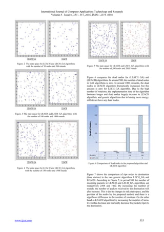
The state space of nodes is displayed as in Figures 2-5 in
LEACH and LECH_GA algorithms, respectively.

3. International Journal of Computer Applications Technology and Research
Volume 5– Issue 6, 353 - 357, 2016, ISSN:- 2319–8656
www.ijcat.com 355
Figure. 2 The state space for LEACH and LECH_GA algorithms
with the number of 50 nodes and 500 rounds
Figure. 3 The state space for LEACH and LECH_GA algorithms with
the number of 100 nodes and 1000 rounds
Figure. 4 The state space for LEACH and LECH_GA algorithms
with the number of 150 nodes and 1500 rounds
Figure. 5 The state space for LEACH and LECH_GA algorithms with
the number of 200 nodes and 2000 rounds
Figure 6 compares the dead nodes for (LEACH GA) and
(LEACH) algorithms. In around 500, the number of dead nodes
in both algorithms is zero. In around 1000 onwards, the dead
nodes in LEACH algorithm dramatically increased, but this
amount is zero for LECH_GA algorithm. Due to the high
number of rotations, the implementation time of the algorithm
becomes longer and dead nodes largely increase in LEACH
algorithm, and genetic algorithms due to having more energy,
still do not have any dead nodes.
Figure. 6 Comparison of dead nodes in the proposed algorithm and
LEACH algorithm
Figure 7 shows the comparison of ripe nodes to destination
(base station) in the two genetic algorithms LECH_GA and
LEACH. According to Figure 7, in period 500 the number of
incoming packets in LEACH and LECH_GA algorithms are
respectively 2508 and 7412. By increasing the number of
rounds, the number of packets received to the destination will
also increase. This is due to changes in sink state space, and the
position of the nodes by the proposed method and there is a
significant difference in the number of rotations. On the other
hand in LEACH algorithm by increasing the number of turns,
live nodes decrease and markedly decrease the packets ripen to
the destination.

4. International Journal of Computer Applications Technology and Research
Volume 5– Issue 6, 353 - 357, 2016, ISSN:- 2319–8656
www.ijcat.com 356
Figure. 7 The number of incoming packets to sink
Figure 8 shows the comparison of the number of choosing
cluster in the two genetic algorithms LECH_GA and LEACH.
In lower revs in the genetic algorithm, no need to select much
cluster, according to the production chromosomes. Also it is
observed that by increasing the rounds, due to high energy
consumption, cluster head with high reliability is chosen for
packet transmission in genetic algorithms.
Figure. 8 Selection of cluster head
Figure 9 shows the comparison of energy consumption for
genetic algorithm, LEACH-GA and LEACH. Energy
consumption for the proposed algorithm has not so declined,
but energy consumption for LEACH algorithm has ended in a
round 2000.
Figure. 9 The remaining energy consumption in both LEACH and
LEACH_GA algorithms
6. CONCLUSION
In this article, congestion control was studied using genetic
algorithms in wireless sensor networks. According to the
results, it was given a new value for the state space of the sink
so that it can have good performance at sending incoming
packets to the destination (sink) when the position (state-space)
of the sink changes, reducing nodes losses, traducing energy
consumption power, selecting better cluster. Whatever the
number of the terms is more in the proposed algorithm, the
performance in terms of dead nodes, number of incoming
packets to the destination and energy would be highly better. A
deep understanding of congestion control lets the transmission
comprehensive protocol design with reliability. Addressing the
transport layer with high reliability is essential to ensure
effectiveness of the applications. Checking the transfer
protocols shows controls of the reliability of a vision to this task
(congestion control).
7. REFERENCES
[1] Akyildiz, I. F., Su, W., Sankarasubramaniam, Y. 2002.
Computer Networks: The International Journal of Computer
and Telecommunications Networking archive Volume 38 Issue
4, 393-422.
[2] Tao, Q. and Yu, F. Q. 210. ECODA: Enhanced Congestion
Detection and Avoidance for Multiple Class of Traffic in
Sensor Networks. in proc. IEEE conf.
[3] Vijayaraja, V. and Hemamalini, R. Congestion in Wireless
Sensor Networks and Various Techniques for Mitigating
Congestion - A Review. in proc. IEEE conf. May2010.
[4] Sridevi, S. Usha, M. and Pauline, G. 2012. Priority Based
CongestionControl For Heterogeneous Traffic In Multipath
Wireless Sensor Networks. inproc. IEEE conf.
[5] Hull, b. jamieson, k. and Balakrishnan, h. 2004. Mitigation
congestion in wireless sensor networks. in procedding of ACM
sensys, vol.4, USA,
[6] Wang, C. and Sohraby, K. 2006. A Survey of Transport
Protocols for Wireless Sensor Networks. IEEE Network,
vol.20, pp.34-40,

5. International Journal of Computer Applications Technology and Research
Volume 5– Issue 6, 353 - 357, 2016, ISSN:- 2319–8656
www.ijcat.com 357
[7] Tezcan, N., and Wang, W. 2007. ART: an asymmetric and
reliable transport mechanism for wireless sensor networks. Int.
J. Sen. Netw, 2(3), 188–200.
[8] Sundaresan, K., Anantharaman, V., Hsieh, H. Y.,
Sivakumar, R. 2005. ATP: A Reliable Transport Protocol for
Ad Hoc Networks. IEEE Trans. Mobile Computing, 4(6), 588–
603.
[9] Kang, J., Zhang, Y., Nath, B. 2007. TARA: Topology-
Aware Resource Adaptation to Alleviate Congestion in Sensor
Networks. IEEE Trans. Parallel Distrib. Syst, 18(7), 919–931.
[10] Wang, G., & Liu, K. 2009. Upstream hop-by-hop
congestion control in wireless sensor networks. in Proc. IEEE
20th Int. Symp. on Personal, Indoor and Mobile Radio
Communications, 1406–1410.
[11] Monowar, M., Rahman, M., Hong, V. S. 2008. Multipath
Congestion Control for Heterogeneous Traffic in Wireless
Sensor Network, in Proc. 10th Int. Conf. on Advanced
Communication Technology, ICACT, 3, 1711–1715.
[12] Mahdizadeh Aghdam, S., Khansari, M. , Rabiee, H. R.,
Salehi, M. 2014. WCCP: A congestion control protocol for
wireless multimedia communication in sensor networks. Ad
Hoc Networks 13 , 516–534.
[13] Gou, H., Yoo, Y., Zeng, H. 2009. A Partition-Based
LEACH Algorithm for Wireless Sensor Networks. CIT '09.
Ninth IEEE International Conference on, Computer and
Information Technology, 2009, IEEE, PP. 40 – 45.
[14] Feigenbaum, J., Kannan, S., McGregor, A., Suri, S. and
Zhang, J. 2005. Graph distances in the streaming model: the
value of space. In ACM-SIAM Symposium on Discrete
Algorithms, 745–754.