The document provides an overview of basic concepts related to parallelization and data locality optimization. It discusses loop-level parallelism as a major target for parallelization, especially in applications using arrays. Long running applications tend to have large arrays, which lead to loops that have many iterations that can be divided among processors. The document also covers data locality and how the organization of computations can significantly impact performance by improving cache usage. It introduces concepts like symmetric multiprocessors and affine transform theory that are useful for parallelization and locality optimizations.


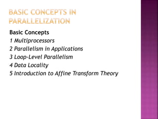
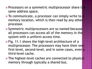
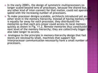
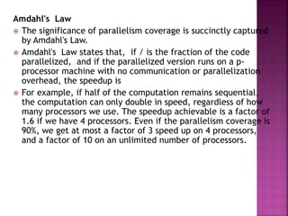
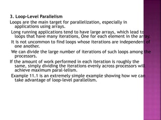
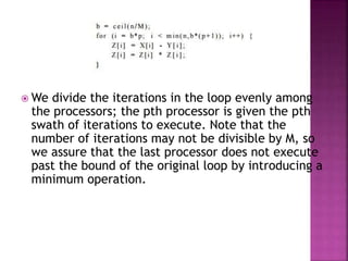
![ Given that the two programs perform the same
computation, which performs better? The fused loop in
Example 11.1 has better performance because it has
better data locality.
Each difference is squared immediately, as soon as it is
produced; in fact, we can hold the difference in a
register, square it, and write the result just once into the
memory location Z[i].
In contrast, the code in Example 11.1 fetches Z[i] once,
and writes it twice. Moreover, if the size of the array is
larger than the cache, Z1i1 needs to be refetched from
memory the second time it is used in this example.
Thus, this code can run significantly slower.](https://image.slidesharecdn.com/compiler-190819133248/85/Compiler-design-28-320.jpg)
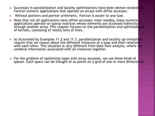
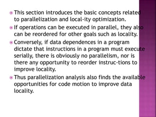
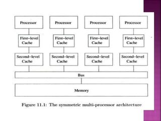
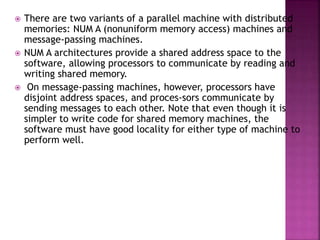
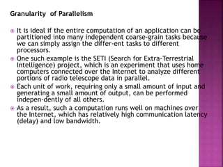
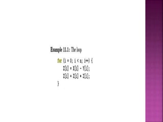
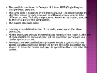
![ 5. Affine Partitioning: We parallelize a loop by using an affine
function to assign iterations in an iteration space to processors in the
processor space.
In our example, we simply assign iteration i to processor i. We can
also specify a new execution order with affine functions. If we wish
to execute the loop above sequentially, but in reverse, we can
specify the ordering function succinctly with an affine expression 10
— i.Thus, iteration 9 is the 1st iteration to execute and so on.
6. Region of Data Accessed: To find the best affine partitioning, it
useful to know the region of data accessed by an iteration.
We can get the region of data accessed by combining the iteration
space information with the array index function. In this case, the
array access Z[i + 10] touches the region {a | 10 < a < 20} and the
access Z[i] touches the region {a10 < a < 10}.](https://image.slidesharecdn.com/compiler-190819133248/85/Compiler-design-38-320.jpg)
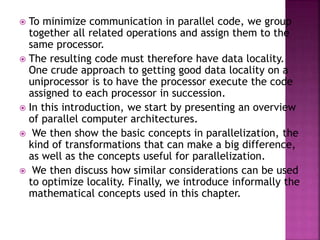
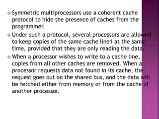
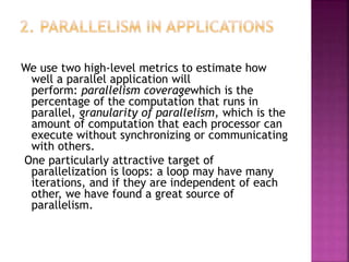
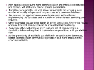
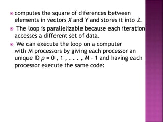
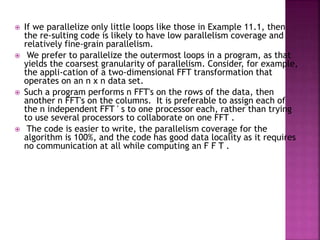
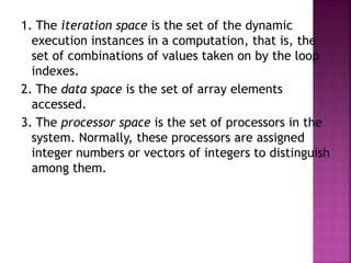
![7. Data Dependence: To determine if the loop is parallelizable, we ask if there is a data
dependence that crosses the boundary of each iteration.
For this example, we first consider the dependences of the write accesses in the
loop. Since the access function Z[z + 10] maps different iterations to differ-ent
array locations, there are no dependences regarding the order in which the various
iterations write values to the array.
Is there a dependence be-tween the read and write accesses? Since only Z[10],
Z[ll],... , Z[19] are written (by the access Z[i + 10]), and only Z[0], Z[l],... , Z[9] are
read (by the access Z[i]), there can be no dependencies regarding the relative order
of a read and a write. Therefore, this loop is parallelizable.
That is, each iteration of the loop is independent of all other iterations, and we
can execute the iterations in parallel, or in any order we choose. Notice, however,
that if we made a small change, say by increasing the upper limit on loop index i to
10 or more, then there would be dependencies, as some elements of array Z would
be written on one iteration and then read 10 iterations later.
In that case, the loop could not be parallelized completely, and we would have to
think carefully about how iterations were partitioned among processors and how we
ordered iterations.](https://image.slidesharecdn.com/compiler-190819133248/85/Compiler-design-39-320.jpg)


![ANIMAL_CELL_,_TISSUE_AND_ORGAN_CULTURE[1].pptx](https://cdn.slidesharecdn.com/ss_thumbnails/animalcelltissueandorganculture1-260204172026-4462b440-thumbnail.jpg?width=640&height=640&fit=bounds)


