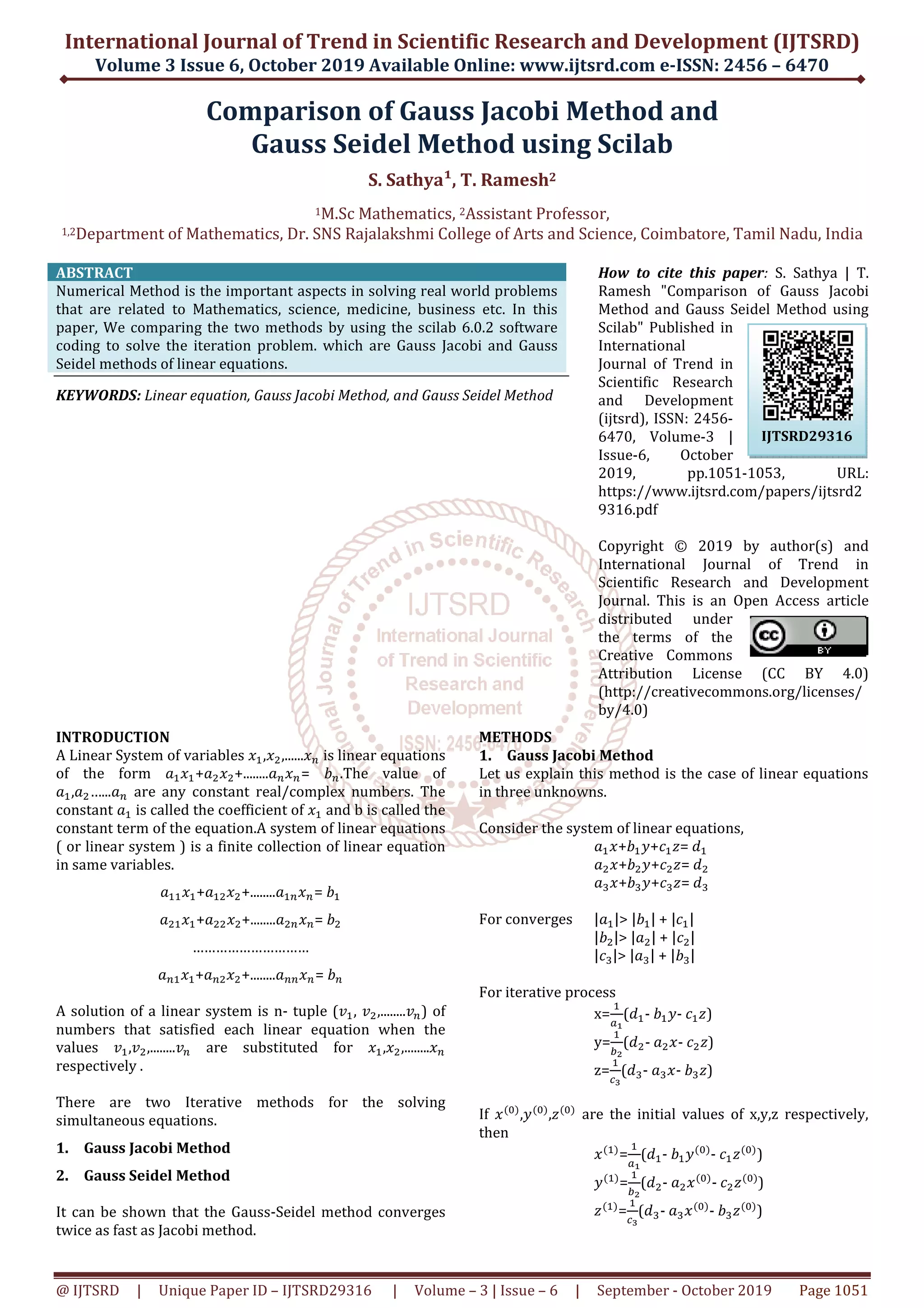
International Journal of Trend in Scientific Research and Development (IJTSRD)
Volume 3 Issue 6, October 2019
@ IJTSRD | Unique Paper ID – IJTSRD293
Comparison
Gauss Seidel Method
1M.Sc Mathematics,
1,2Department of Mathematics, Dr. SNS Rajalakshmi
ABSTRACT
Numerical Method is the important aspects in solving real world problems
that are related to Mathematics, science,
paper, We comparing the two methods by using the scilab 6.0.2 software
coding to solve the iteration problem. which are Gauss Jacobi and Gauss
Seidel methods of linear equations.
KEYWORDS: Linear equation, Gauss Jacobi Method, and Gauss Seidel
INTRODUCTION
A Linear System of variables ‫ݔ‬ଵ,‫ݔ‬ଶ,......‫ݔ‬௡ is linear equations
of the form ܽଵ‫ݔ‬ଵ+ܽଶ‫ݔ‬ଶ+........ܽ௡‫ݔ‬௡= ܾ௡
ܽଵ,ܽଶ…...ܽ௡ are any constant real/complex numbers. The
constant ܽଵ is called the coefficient of ‫ݔ‬ଵ and b is called the
constant term of the equation.A system of linear equations
( or linear system ) is a finite collection of linear equation
in same variables.
ܽଵଵ‫ݔ‬ଵ+ܽଵଶ‫ݔ‬ଶ+........ܽଵ௡‫ݔ‬௡= ܾଵ
ܽଶଵ‫ݔ‬ଵ+ܽଶଶ‫ݔ‬ଶ+........ܽଶ௡‫ݔ‬௡= ܾ
…………………………
ܽ௡ଵ‫ݔ‬ଵ+ܽ௡ଶ‫ݔ‬ଶ+........ܽ௡௡‫ݔ‬௡= ܾ
A solution of a linear system is n- tuple (
numbers that satisfied each linear equation when the
values ‫ݒ‬ଵ,‫ݒ‬ଶ,........‫ݒ‬௡ are substituted for
respectively .
There are two Iterative methods for the solving
simultaneous equations.
1. Gauss Jacobi Method
2. Gauss Seidel Method
It can be shown that the Gauss-Seidel method converges
twice as fast as Jacobi method.
International Journal of Trend in Scientific Research and Development (IJTSRD)
2019 Available Online: www.ijtsrd.com e
29316 | Volume – 3 | Issue – 6 | September
Comparison of Gauss Jacobi Method
Gauss Seidel Method using Scilab
S. Sathya¹, T. Ramesh2
M.Sc Mathematics, 2Assistant Professor,
SNS Rajalakshmi College of Arts and Science, Coimbatore,
Numerical Method is the important aspects in solving real world problems
science, medicine, business etc. In this
We comparing the two methods by using the scilab 6.0.2 software
on problem. which are Gauss Jacobi and Gauss
Gauss Jacobi Method, and Gauss Seidel Method
How to cite this paper
Ramesh "Comparison of Gauss Jacobi
Method and Gauss Seidel Method using
Scilab" Published in
International
Journal of Trend in
Scientific Research
and Development
(ijtsrd), ISSN: 2456
6470, Volume
Issue-6, October
2019, pp.1051
https://www.ijtsrd.com/papers/ijtsrd2
9316.pdf
Copyright © 2019 by author(s) and
International Journal of Trend in
Scientific Research and Development
Journal. This is an Open Access article
distributed under
the terms of the
Creative Commons
Attribution License (CC BY 4.0)
(http://creativecommons.org/licenses/
by/4.0)
is linear equations
௡.The value of
any constant real/complex numbers. The
and b is called the
constant term of the equation.A system of linear equations
( or linear system ) is a finite collection of linear equation
ܾଵ
ܾଶ
ܾ௡
tuple (‫ݒ‬ଵ, ‫ݒ‬ଶ,........‫ݒ‬௡) of
numbers that satisfied each linear equation when the
are substituted for ‫ݔ‬ଵ,‫ݔ‬ଶ,........‫ݔ‬௡
There are two Iterative methods for the solving
Seidel method converges
METHODS
1. Gauss Jacobi Method
Let us explain this method is the case of linear equations
in three unknowns.
Consider the system of linear equations,
ܽଵ‫ܾ+ݔ‬ଵ‫ܿ+ݕ‬ଵ
ܽଶ‫ܾ+ݔ‬ଶ‫ܿ+ݕ‬ଶ
ܽଷ‫ܾ+ݔ‬ଷ‫ܿ+ݕ‬ଷ
For converges |ܽଵ|> |ܾଵ| +
|ܾଶ|> |ܽଶ| +
|ܿଷ|> |ܽଷ| +
For iterative process
x=
ଵ
௔భ
(݀ଵ- ܾଵ‫ݕ‬
y=
ଵ
௕మ
(݀ଶ- ܽଶ
z=
ଵ
௖య
(݀ଷ- ܽଷ‫ݔ‬
If ‫ݔ‬ሺ଴ሻ
,‫ݕ‬ሺ଴ሻ
,‫ݖ‬ሺ଴ሻ
are the initial values of x,y,z respectively,
then
‫ݔ‬ሺଵሻ
=
ଵ
௔భ
(݀ଵ-
‫ݕ‬ሺଵሻ
=
ଵ
௕మ
(݀ଶ-
‫ݖ‬ሺଵሻ
=
ଵ
௖య
(݀ଷ-
International Journal of Trend in Scientific Research and Development (IJTSRD)
e-ISSN: 2456 – 6470
6 | September - October 2019 Page 1051
f Gauss Jacobi Method and
sing Scilab
Coimbatore, Tamil Nadu, India
How to cite this paper: S. Sathya | T.
Ramesh "Comparison of Gauss Jacobi
Method and Gauss Seidel Method using
Scilab" Published in
International
Journal of Trend in
Scientific Research
and Development
(ijtsrd), ISSN: 2456-
6470, Volume-3 |
6, October
2019, pp.1051-1053, URL:
https://www.ijtsrd.com/papers/ijtsrd2
Copyright © 2019 by author(s) and
International Journal of Trend in
Scientific Research and Development
Journal. This is an Open Access article
distributed under
the terms of the
Creative Commons
Attribution License (CC BY 4.0)
http://creativecommons.org/licenses/
Let us explain this method is the case of linear equations
Consider the system of linear equations,
ଵ‫=ݖ‬ ݀ଵ
ଶ‫=ݖ‬ ݀ଶ
ଷ‫=ݖ‬ ݀ଷ
|ܿଵ|
|ܿଶ|
|ܾଷ|
‫-ݕ‬ ܿଵ‫)ݖ‬
ଶ‫-ݔ‬ ܿଶ‫)ݖ‬
‫-ݔ‬ ܾଷ‫)ݖ‬
are the initial values of x,y,z respectively,
ܾଵ‫ݕ‬ሺ଴ሻ
- ܿଵ‫ݖ‬ሺ଴ሻ
)
ܽଶ‫ݔ‬ሺ଴ሻ
- ܿଶ‫ݖ‬ሺ଴ሻ
)
ܽଷ‫ݔ‬ሺ଴ሻ
- ܾଷ‫ݖ‬ሺ଴ሻ
)
IJTSRD29316
International Journal of Trend in Scientific Research and Development (IJTSRD) @ www.ijtsrd.com eISSN: 2456-6470
@ IJTSRD | Unique Paper ID – IJTSRD29316 | Volume – 3 | Issue – 6 | September - October 2019 Page 1052
Again using these value ‫ݔ‬ሺଵሻ
,‫ݕ‬ሺଵሻ
,‫ݖ‬ሺଵሻ
we get
‫ݔ‬ሺଶሻ
=
ଵ
௔భ
(݀ଵ- ܾଵ‫ݕ‬ሺଵሻ
- ܿଵ‫ݖ‬ሺଵሻ
)
‫ݕ‬ሺଶሻ
=
ଵ
௕మ
(݀ଶ- ܽଶ‫ݔ‬ሺଵሻ
- ܿଶ‫ݖ‬ሺଵሻ
)
‫ݖ‬ሺଶሻ
=
ଵ
௖య
(݀ଷ- ܽଷ‫ݔ‬ሺଵሻ
- ܾଷ‫ݖ‬ሺଵሻ
)
Proceeding in the same way , if the rth iterates are
‫ݔ‬ሺ௥ሻ
,‫ݕ‬ሺ௥ሻ
,‫ݖ‬ሺ௥ሻ
, the iteration scheme reduces to
‫ݔ‬ሺ௥ାଵሻ
=
ଵ
௔భ
(݀ଵ- ܾଵ‫ݕ‬ሺ௥ሻ
- ܿଵ‫ݖ‬ሺ௥ሻ
)
‫ݕ‬ሺ௥ାଵሻ
=
ଵ
௕మ
(݀ଶ- ܽଶ‫ݔ‬ሺ௥ሻ
- ܿଶ‫ݖ‬ሺ௥ሻ
)
‫ݖ‬ሺ௥ାଵሻ
=
ଵ
௖య
(݀ଷ- ܽଷ‫ݔ‬ሺ௥ሻ
- ܾଷ‫ݖ‬ሺ௥ሻ
)
The procedure is continued till the convergence is assured
(correct to required decimals).
PROBLEM: Solve the following equation by Gauss
Jacobi Method.
10x-5y-2z=3; 4x-10y+3z=-3; x+6y+10z=-3.
Solution:
The below result is find out by the manual work:
n X y z
1 0.3 0.3 -0.3
2 0.39 0.33 -0.51
3 0.363 0.303 -0.537
4 0.3441 0.2841 -0.5181
5 0.33843 0.2822 -0.50487
6 0.340126 0.283911 -0.503163
7 0.3413229 0.2851015 -0.5043592
8 0.34167891 0.2852214 -0.50519319
9 0.341572062 0.285113607 -0.505300731
By using Scilab coding the result shown below:
n X y z
1 0.3 0.3 -0.3
2 0.39 0.33 -0.51
3 0.363 0.303 -0.537
4 0.3441 0.2841 -0.5181
5 0.33843 0.28221 -0.50487
6 0.340131 0.283911 -0.503169
7 0.341322 0.285102 -0.50436
8 0.341679 0.285221 -0.505193
9 0.341572 0.285114 -0.5053
The Actual Values are x=0.3415, y=0.2852, and
z=−0.5053.
2. Gauss-Seidel Method
This is only a refinement of Gauss-Jacobi Method As
before,
x=
ଵ
௔భ
(݀ଵ- ܾଵ‫-ݕ‬ ܿଵ‫)ݖ‬
y=
ଵ
௕మ
(݀ଶ- ܽଶ‫-ݔ‬ ܿଶ‫)ݖ‬
z=
ଵ
௖య
(݀ଷ- ܽଷ‫-ݔ‬ ܾଷ‫)ݕ‬
We start with the initial values ‫ݕ‬ሺ଴ሻ
,‫ݖ‬ሺ଴ሻ
for y and z and get
‫ݔ‬ሺଵሻ
That is,
‫ݔ‬ሺଵሻ
=
ଵ
௔భ
(݀ଵ- ܾଵ‫ݕ‬ሺ଴ሻ
- ܿଵ‫ݖ‬ሺ଴ሻ
)
We use ‫ݖ‬ሺ଴ሻ
for z and ‫ݔ‬ሺଵሻ
for x instead of ‫ݔ‬ሺ଴ሻ
as in the
Jacobi’s Method, we get
‫ݕ‬ሺଵሻ
=
ଵ
௕మ
(݀ଶ- ܽଶ‫ݕ‬ሺଵሻ
- ܿଶ‫ݖ‬ሺ଴ሻ
)
Now , having known ‫ݔ‬ሺଵሻ
and ‫ݕ‬ሺଵሻ
use ‫ݔ‬ሺଵሻ
for x and ‫ݕ‬ሺଵሻ
for
y ,we get
‫ݖ‬ሺଵሻ
=
ଵ
௖య
(݀ଷ- ܽଷ‫ݔ‬ሺଵሻ
- ܾଷ‫ݕ‬ଵ
)
In finding the values of the unknowns, we use the latest
available values on the right hand side. If ‫ݔ‬ሺ௥ሻ
,‫ݕ‬ሺ௥ሻ
,‫ݖ‬ሺ௥ሻ
are
the rth iterates , then the iterates scheme will be
‫ݔ‬ሺ௥ାଵሻ
=
ଵ
௔భ
(݀ଵ- ܾଵ‫ݕ‬ሺ௥ሻ
- ܿଵ‫ݖ‬ሺ௥ሻ
)
‫ݕ‬ሺ௥ାଵሻ
=
ଵ
௕మ
(݀ଶ- ܽଶ‫ݔ‬ሺ௥ାଵሻ
- ܿଶ‫ݖ‬ሺ௥ሻ
)
‫ݖ‬ሺ௥ାଵሻ
=
ଵ
௖య
(݀ଷ- ܽଷ‫ݔ‬ሺ௥ାଵሻ
- ܾଷ‫ݕ‬ሺ௥ାଵሻ
)
This Process of iteration is continued until the
convergence is assured.
PROBLEM: Solve the following equation by Gauss-
Seidel Method.
10x-5y-2z=3; 4x-10y+3z=-3; x+6y+10z=-3.
Solution:
The result is find out by the manual work.
N x y z
1 0.3 0.42 -0.582
2 0.3936 0.28284 -0.509064
3 0.3396072 0.28312364 -0.503834928
4 0.34079485 0.28516746 -0.50517996
5 0.3415547 0.28506792 -0.505196229
6 0.3414947 0.285039 -0.5051728
7 0.3414849 0.28504212 -0.5051737
By using the Scilab coding the result is shown below:
International Journal of Trend in Scientific Research and Development (IJTSRD) @ www.ijtsrd.com eISSN: 2456-6470
@ IJTSRD | Unique Paper ID – IJTSRD29316 | Volume – 3 | Issue – 6 | September - October 2019 Page 1053
N x y z
1 0.3 0.42 -0.582
2 0.3936 0.28284 -0.509064
3 0.33960 0.283124 -0.503835
4 0.340795 0.285167 -0.50518
5 0.341548 0.285065 -0.505194
6 0.341494 0.285039 -0.505173
7 0.341485 0.285042 -0.505174
The Actual value are x=0.3415, y=0.2852, and z= -
0.5053.
CONCLUSION
There are different methods of solving of linear equation
some are direct methods while some are iterative
methods. In this paper , two Iteration methods of solving
of linear equation have been presented where the Gauss-
Seidel Method proved to be the best and effective in the
sense that it converge very fast with Scilab Software.
REFERENCE
[1] P. Kandhasamy, K. Thilagavathy and K. Gunavathi
”Numerical Methods”, book.
[2] Atendra singh yadav, Ashik kumar,”Numerical
Solution Of System Of Linear Equation By Iterative
Methods”, journal,2017.
[3] Abubakkar siddiq, R. Lavanya, V. S. Akilandeswari,
”Modified Gauss Elimination Method”,journal,2017
[4] Udai Bhan Trivedi, Sandosh Kumar, Vishok Kumar
Singh,”Gauss Elimination, Gauss Jordan and Gauss
Seidel Iteration Method: Performance Comparison
Using MATLAB”,2017.
[5] Zhang Lijuan, Guan Tianye, Comparison Of Several
Numerical Algorithm For Solving Ordinary
Differential Equation Initial Value Problem, 2018.

Comparison of Gauss Jacobi Method and Gauss Seidel Method using Scilab

  • 1.
    International Journal ofTrend in Scientific Research and Development (IJTSRD) Volume 3 Issue 6, October 2019 @ IJTSRD | Unique Paper ID – IJTSRD293 Comparison Gauss Seidel Method 1M.Sc Mathematics, 1,2Department of Mathematics, Dr. SNS Rajalakshmi ABSTRACT Numerical Method is the important aspects in solving real world problems that are related to Mathematics, science, paper, We comparing the two methods by using the scilab 6.0.2 software coding to solve the iteration problem. which are Gauss Jacobi and Gauss Seidel methods of linear equations. KEYWORDS: Linear equation, Gauss Jacobi Method, and Gauss Seidel INTRODUCTION A Linear System of variables ‫ݔ‬ଵ,‫ݔ‬ଶ,......‫ݔ‬௡ is linear equations of the form ܽଵ‫ݔ‬ଵ+ܽଶ‫ݔ‬ଶ+........ܽ௡‫ݔ‬௡= ܾ௡ ܽଵ,ܽଶ…...ܽ௡ are any constant real/complex numbers. The constant ܽଵ is called the coefficient of ‫ݔ‬ଵ and b is called the constant term of the equation.A system of linear equations ( or linear system ) is a finite collection of linear equation in same variables. ܽଵଵ‫ݔ‬ଵ+ܽଵଶ‫ݔ‬ଶ+........ܽଵ௡‫ݔ‬௡= ܾଵ ܽଶଵ‫ݔ‬ଵ+ܽଶଶ‫ݔ‬ଶ+........ܽଶ௡‫ݔ‬௡= ܾ ………………………… ܽ௡ଵ‫ݔ‬ଵ+ܽ௡ଶ‫ݔ‬ଶ+........ܽ௡௡‫ݔ‬௡= ܾ A solution of a linear system is n- tuple ( numbers that satisfied each linear equation when the values ‫ݒ‬ଵ,‫ݒ‬ଶ,........‫ݒ‬௡ are substituted for respectively . There are two Iterative methods for the solving simultaneous equations. 1. Gauss Jacobi Method 2. Gauss Seidel Method It can be shown that the Gauss-Seidel method converges twice as fast as Jacobi method. International Journal of Trend in Scientific Research and Development (IJTSRD) 2019 Available Online: www.ijtsrd.com e 29316 | Volume – 3 | Issue – 6 | September Comparison of Gauss Jacobi Method Gauss Seidel Method using Scilab S. Sathya¹, T. Ramesh2 M.Sc Mathematics, 2Assistant Professor, SNS Rajalakshmi College of Arts and Science, Coimbatore, Numerical Method is the important aspects in solving real world problems science, medicine, business etc. In this We comparing the two methods by using the scilab 6.0.2 software on problem. which are Gauss Jacobi and Gauss Gauss Jacobi Method, and Gauss Seidel Method How to cite this paper Ramesh "Comparison of Gauss Jacobi Method and Gauss Seidel Method using Scilab" Published in International Journal of Trend in Scientific Research and Development (ijtsrd), ISSN: 2456 6470, Volume Issue-6, October 2019, pp.1051 https://www.ijtsrd.com/papers/ijtsrd2 9316.pdf Copyright © 2019 by author(s) and International Journal of Trend in Scientific Research and Development Journal. This is an Open Access article distributed under the terms of the Creative Commons Attribution License (CC BY 4.0) (http://creativecommons.org/licenses/ by/4.0) is linear equations ௡.The value of any constant real/complex numbers. The and b is called the constant term of the equation.A system of linear equations ( or linear system ) is a finite collection of linear equation ܾଵ ܾଶ ܾ௡ tuple (‫ݒ‬ଵ, ‫ݒ‬ଶ,........‫ݒ‬௡) of numbers that satisfied each linear equation when the are substituted for ‫ݔ‬ଵ,‫ݔ‬ଶ,........‫ݔ‬௡ There are two Iterative methods for the solving Seidel method converges METHODS 1. Gauss Jacobi Method Let us explain this method is the case of linear equations in three unknowns. Consider the system of linear equations, ܽଵ‫ܾ+ݔ‬ଵ‫ܿ+ݕ‬ଵ ܽଶ‫ܾ+ݔ‬ଶ‫ܿ+ݕ‬ଶ ܽଷ‫ܾ+ݔ‬ଷ‫ܿ+ݕ‬ଷ For converges |ܽଵ|> |ܾଵ| + |ܾଶ|> |ܽଶ| + |ܿଷ|> |ܽଷ| + For iterative process x= ଵ ௔భ (݀ଵ- ܾଵ‫ݕ‬ y= ଵ ௕మ (݀ଶ- ܽଶ z= ଵ ௖య (݀ଷ- ܽଷ‫ݔ‬ If ‫ݔ‬ሺ଴ሻ ,‫ݕ‬ሺ଴ሻ ,‫ݖ‬ሺ଴ሻ are the initial values of x,y,z respectively, then ‫ݔ‬ሺଵሻ = ଵ ௔భ (݀ଵ- ‫ݕ‬ሺଵሻ = ଵ ௕మ (݀ଶ- ‫ݖ‬ሺଵሻ = ଵ ௖య (݀ଷ- International Journal of Trend in Scientific Research and Development (IJTSRD) e-ISSN: 2456 – 6470 6 | September - October 2019 Page 1051 f Gauss Jacobi Method and sing Scilab Coimbatore, Tamil Nadu, India How to cite this paper: S. Sathya | T. Ramesh "Comparison of Gauss Jacobi Method and Gauss Seidel Method using Scilab" Published in International Journal of Trend in Scientific Research and Development (ijtsrd), ISSN: 2456- 6470, Volume-3 | 6, October 2019, pp.1051-1053, URL: https://www.ijtsrd.com/papers/ijtsrd2 Copyright © 2019 by author(s) and International Journal of Trend in Scientific Research and Development Journal. This is an Open Access article distributed under the terms of the Creative Commons Attribution License (CC BY 4.0) http://creativecommons.org/licenses/ Let us explain this method is the case of linear equations Consider the system of linear equations, ଵ‫=ݖ‬ ݀ଵ ଶ‫=ݖ‬ ݀ଶ ଷ‫=ݖ‬ ݀ଷ |ܿଵ| |ܿଶ| |ܾଷ| ‫-ݕ‬ ܿଵ‫)ݖ‬ ଶ‫-ݔ‬ ܿଶ‫)ݖ‬ ‫-ݔ‬ ܾଷ‫)ݖ‬ are the initial values of x,y,z respectively, ܾଵ‫ݕ‬ሺ଴ሻ - ܿଵ‫ݖ‬ሺ଴ሻ ) ܽଶ‫ݔ‬ሺ଴ሻ - ܿଶ‫ݖ‬ሺ଴ሻ ) ܽଷ‫ݔ‬ሺ଴ሻ - ܾଷ‫ݖ‬ሺ଴ሻ ) IJTSRD29316
  • 2.
    International Journal ofTrend in Scientific Research and Development (IJTSRD) @ www.ijtsrd.com eISSN: 2456-6470 @ IJTSRD | Unique Paper ID – IJTSRD29316 | Volume – 3 | Issue – 6 | September - October 2019 Page 1052 Again using these value ‫ݔ‬ሺଵሻ ,‫ݕ‬ሺଵሻ ,‫ݖ‬ሺଵሻ we get ‫ݔ‬ሺଶሻ = ଵ ௔భ (݀ଵ- ܾଵ‫ݕ‬ሺଵሻ - ܿଵ‫ݖ‬ሺଵሻ ) ‫ݕ‬ሺଶሻ = ଵ ௕మ (݀ଶ- ܽଶ‫ݔ‬ሺଵሻ - ܿଶ‫ݖ‬ሺଵሻ ) ‫ݖ‬ሺଶሻ = ଵ ௖య (݀ଷ- ܽଷ‫ݔ‬ሺଵሻ - ܾଷ‫ݖ‬ሺଵሻ ) Proceeding in the same way , if the rth iterates are ‫ݔ‬ሺ௥ሻ ,‫ݕ‬ሺ௥ሻ ,‫ݖ‬ሺ௥ሻ , the iteration scheme reduces to ‫ݔ‬ሺ௥ାଵሻ = ଵ ௔భ (݀ଵ- ܾଵ‫ݕ‬ሺ௥ሻ - ܿଵ‫ݖ‬ሺ௥ሻ ) ‫ݕ‬ሺ௥ାଵሻ = ଵ ௕మ (݀ଶ- ܽଶ‫ݔ‬ሺ௥ሻ - ܿଶ‫ݖ‬ሺ௥ሻ ) ‫ݖ‬ሺ௥ାଵሻ = ଵ ௖య (݀ଷ- ܽଷ‫ݔ‬ሺ௥ሻ - ܾଷ‫ݖ‬ሺ௥ሻ ) The procedure is continued till the convergence is assured (correct to required decimals). PROBLEM: Solve the following equation by Gauss Jacobi Method. 10x-5y-2z=3; 4x-10y+3z=-3; x+6y+10z=-3. Solution: The below result is find out by the manual work: n X y z 1 0.3 0.3 -0.3 2 0.39 0.33 -0.51 3 0.363 0.303 -0.537 4 0.3441 0.2841 -0.5181 5 0.33843 0.2822 -0.50487 6 0.340126 0.283911 -0.503163 7 0.3413229 0.2851015 -0.5043592 8 0.34167891 0.2852214 -0.50519319 9 0.341572062 0.285113607 -0.505300731 By using Scilab coding the result shown below: n X y z 1 0.3 0.3 -0.3 2 0.39 0.33 -0.51 3 0.363 0.303 -0.537 4 0.3441 0.2841 -0.5181 5 0.33843 0.28221 -0.50487 6 0.340131 0.283911 -0.503169 7 0.341322 0.285102 -0.50436 8 0.341679 0.285221 -0.505193 9 0.341572 0.285114 -0.5053 The Actual Values are x=0.3415, y=0.2852, and z=−0.5053. 2. Gauss-Seidel Method This is only a refinement of Gauss-Jacobi Method As before, x= ଵ ௔భ (݀ଵ- ܾଵ‫-ݕ‬ ܿଵ‫)ݖ‬ y= ଵ ௕మ (݀ଶ- ܽଶ‫-ݔ‬ ܿଶ‫)ݖ‬ z= ଵ ௖య (݀ଷ- ܽଷ‫-ݔ‬ ܾଷ‫)ݕ‬ We start with the initial values ‫ݕ‬ሺ଴ሻ ,‫ݖ‬ሺ଴ሻ for y and z and get ‫ݔ‬ሺଵሻ That is, ‫ݔ‬ሺଵሻ = ଵ ௔భ (݀ଵ- ܾଵ‫ݕ‬ሺ଴ሻ - ܿଵ‫ݖ‬ሺ଴ሻ ) We use ‫ݖ‬ሺ଴ሻ for z and ‫ݔ‬ሺଵሻ for x instead of ‫ݔ‬ሺ଴ሻ as in the Jacobi’s Method, we get ‫ݕ‬ሺଵሻ = ଵ ௕మ (݀ଶ- ܽଶ‫ݕ‬ሺଵሻ - ܿଶ‫ݖ‬ሺ଴ሻ ) Now , having known ‫ݔ‬ሺଵሻ and ‫ݕ‬ሺଵሻ use ‫ݔ‬ሺଵሻ for x and ‫ݕ‬ሺଵሻ for y ,we get ‫ݖ‬ሺଵሻ = ଵ ௖య (݀ଷ- ܽଷ‫ݔ‬ሺଵሻ - ܾଷ‫ݕ‬ଵ ) In finding the values of the unknowns, we use the latest available values on the right hand side. If ‫ݔ‬ሺ௥ሻ ,‫ݕ‬ሺ௥ሻ ,‫ݖ‬ሺ௥ሻ are the rth iterates , then the iterates scheme will be ‫ݔ‬ሺ௥ାଵሻ = ଵ ௔భ (݀ଵ- ܾଵ‫ݕ‬ሺ௥ሻ - ܿଵ‫ݖ‬ሺ௥ሻ ) ‫ݕ‬ሺ௥ାଵሻ = ଵ ௕మ (݀ଶ- ܽଶ‫ݔ‬ሺ௥ାଵሻ - ܿଶ‫ݖ‬ሺ௥ሻ ) ‫ݖ‬ሺ௥ାଵሻ = ଵ ௖య (݀ଷ- ܽଷ‫ݔ‬ሺ௥ାଵሻ - ܾଷ‫ݕ‬ሺ௥ାଵሻ ) This Process of iteration is continued until the convergence is assured. PROBLEM: Solve the following equation by Gauss- Seidel Method. 10x-5y-2z=3; 4x-10y+3z=-3; x+6y+10z=-3. Solution: The result is find out by the manual work. N x y z 1 0.3 0.42 -0.582 2 0.3936 0.28284 -0.509064 3 0.3396072 0.28312364 -0.503834928 4 0.34079485 0.28516746 -0.50517996 5 0.3415547 0.28506792 -0.505196229 6 0.3414947 0.285039 -0.5051728 7 0.3414849 0.28504212 -0.5051737 By using the Scilab coding the result is shown below:
  • 3.
    International Journal ofTrend in Scientific Research and Development (IJTSRD) @ www.ijtsrd.com eISSN: 2456-6470 @ IJTSRD | Unique Paper ID – IJTSRD29316 | Volume – 3 | Issue – 6 | September - October 2019 Page 1053 N x y z 1 0.3 0.42 -0.582 2 0.3936 0.28284 -0.509064 3 0.33960 0.283124 -0.503835 4 0.340795 0.285167 -0.50518 5 0.341548 0.285065 -0.505194 6 0.341494 0.285039 -0.505173 7 0.341485 0.285042 -0.505174 The Actual value are x=0.3415, y=0.2852, and z= - 0.5053. CONCLUSION There are different methods of solving of linear equation some are direct methods while some are iterative methods. In this paper , two Iteration methods of solving of linear equation have been presented where the Gauss- Seidel Method proved to be the best and effective in the sense that it converge very fast with Scilab Software. REFERENCE [1] P. Kandhasamy, K. Thilagavathy and K. Gunavathi ”Numerical Methods”, book. [2] Atendra singh yadav, Ashik kumar,”Numerical Solution Of System Of Linear Equation By Iterative Methods”, journal,2017. [3] Abubakkar siddiq, R. Lavanya, V. S. Akilandeswari, ”Modified Gauss Elimination Method”,journal,2017 [4] Udai Bhan Trivedi, Sandosh Kumar, Vishok Kumar Singh,”Gauss Elimination, Gauss Jordan and Gauss Seidel Iteration Method: Performance Comparison Using MATLAB”,2017. [5] Zhang Lijuan, Guan Tianye, Comparison Of Several Numerical Algorithm For Solving Ordinary Differential Equation Initial Value Problem, 2018.