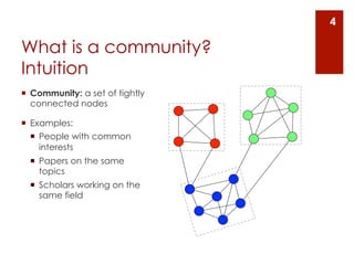
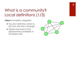
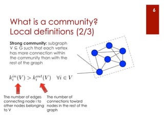
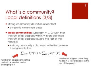
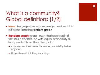
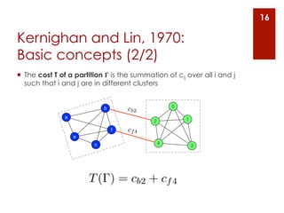
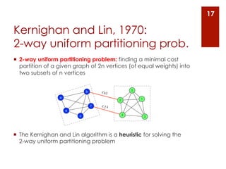
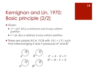
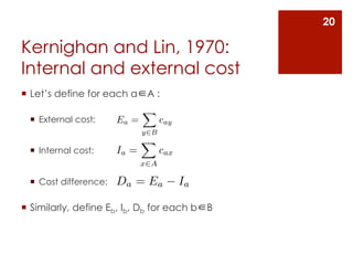
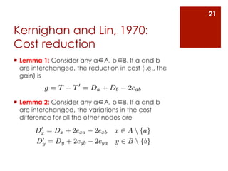
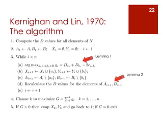
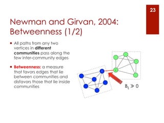
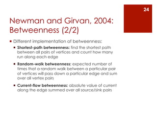
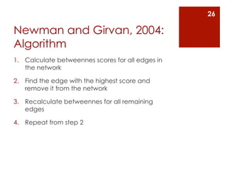
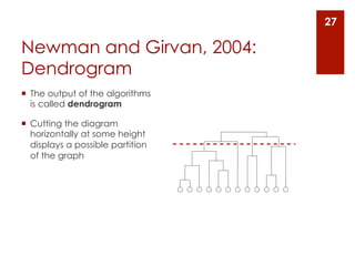
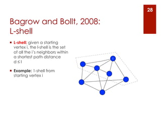
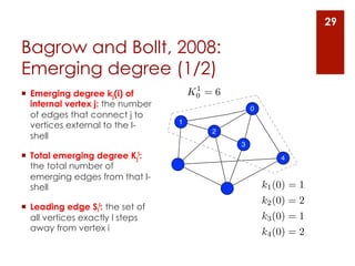
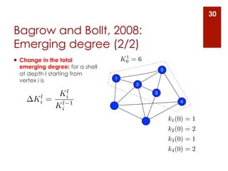
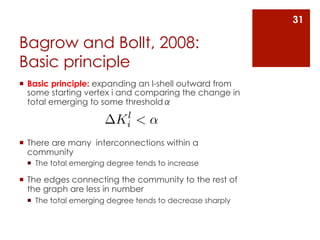
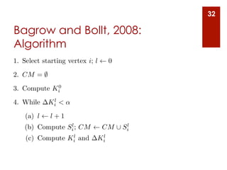
The document provides an overview of community detection in networks. It defines what a community and partition are, and describes several algorithms for partitioning networks into communities: 1. Kernighan and Lin's algorithm from 1970 which iteratively swaps nodes between partitions to minimize the cost. 2. Newman and Girvan's algorithm from 2004 which removes the edge with the highest betweenness centrality on each iteration. 3. Bagrow and Bollt's algorithm from 2008 which expands a shell of nodes out from a seed node, looking for a drop in the total emerging degree to identify community boundaries. The document also discusses different ways to define communities, assess partition quality, and represent partitioning results as a dendrogram

1. Community Detection
Ilio Catallo, catallo@elet.polimi.it
Politecnico di Milano

2. Outline
¡ Communities and Partitions
¡ What is a community?
¡ What is a partition?
¡ Partitioning algorithms
¡ Kerninghan and Lin, 1970
¡ Newman and Girvan, 2004
¡ Bagrow and Bollt, 2008
¡ Assess the quality of good partitions
¡ The impossibility theorem
¡ Quality functions

3. Communities
and
Partitions

4. 4
What is a community?
Intuition
¡ Community: a set of tightly
connected nodes
¡ Examples:
¡ People with common
interests
¡ Papers on the same
topics
¡ Scholars working on the
same field

5. 5
What is a community?
Local definitions (1/3)
clique (complete subgraph)
¡ Too strict definition (what to
do if just one link is missing?)
¡ Cliques are hard to find
(exponential complexity in
the graph size)

6. 6
What is a community?
Local definitions (2/3)
Strong community: subgraph
V ⊆ G such that each vertex
has more connection within
the community than with the
rest of the graph
in out
ki (V ) > ki (V ) 8i 2 V
The number of edges The number of
connecting node i to connections toward
other nodes belonging nodes in the rest of the
to V graph

7. 7
What is a community?
Local definitions (3/3)
¡ Strong communitiy definition is too strict
¡ Unrealistic in many real cases
¡ Weak communities: subgraph V ⊆ G such that
the sum of all degrees within V in greater than
the sum of all degrees toward the rest of the
network
¡ A strong community is also weak, while the converse
is not generally true
P in
P out
i2V ki (V )> i2V ki (V )
number of edges connecting
number of edges connecting nodes in V toward nodes in the
nodes in V to other nodes rest of the graph
belonging to V

8. 8
What is a community?
Global definitions (1/2)
¡ Idea: the graph has a community structure if it is
different from the random graph
¡ Random graph: graph such that each pair of
vertices is connected with equal probability p,
independently on the other pairs
¡ Any two vertices have the same probability to be
adjacent
¡ No preferential linking involving

9. 9
What is a community?
Global definitions (2/2)
¡ The graph of interest is compared with the null
model
¡ Null model: a graph which matches the original
in some of its structural features, but which is
otherwise a random graph
¡ Used as term of comparison to verify whether the
graph of interest shows community structures

10. 10
What is a community?
Vertex-based definitions
¡ Idea: communities are subgraphs of vertices similar
to each other
¡ A measure of similarity needs to be defined
¡ If it is possible to embed the vertices in an n-
dimensional Euclidian space, possible (dis)similarity
measures are: q
PN 2
¡ Euclidian distance dA,B = j (ak bk )
PN 2
¡ Manhattan distance dA,B = j |(ak bk ) |
A·B
¡ Cosine similarity dA,B = kAkkBk
¡ With A = (a1, a2, …, aN) and B = (b1, b2, …, bN) vertex
feature vectors

11. 11
What is a community?
Vertex-based definitions
¡ If it is not possible to embed the vertices in
Euclidian space the similarity must be inferred
from the adjacency relationships
¡ Dissimilarity measure based on structural
equivalence:
qP
dij = k6=i,j (Aik Ajk )2
¡ Structural equivalence: two vertices are structural
equivalent if they have the same neighbors,
even if they are not adjacent themselves
¡ if i and j are structural equivalent then dij = 0

12. 12
What is a partition?
¡ Partition: a division of a
graph in clusters, such that
each vertex belongs to one
cluster
¡ If the vertices can be
shared among different
communities the division is
called cover

13. 13
How many partitions we
may have in a graph?
¡ Stirling number of second kind: the number of
possible partitions in k clusters of a graph with n
vertices
⇢
1 k = n, k = 1
S(n, k) =
kS(n 1, k) + S(n 1, k 1) otherwise
¡ Nth Bell number: the total number of possible
partitions n
X
Bn = S(n, k)
k=1
¡ The nth Bell number is huge, even for relatively
small graphs

14. Partitioning
algorithms

15. 15
Kernighan and Lin, 1970:
Basic concepts (1/2)
¡ Given:
¡ A graph G = (N,A) of n vertices of weights wi > 0
¡ p a positive number s.t. wi ≤ p
¡ C = (cij) the weighted adjacency matrix (cost matrix)
¡ A k-way partition 𝚪 of G is a set of non-empty,
pairwise disjoint set 𝜐1, …, 𝜐k such that:
k
[
i =G
i=1
The sum of weights of
¡ A partition is admissible if: vertices in 𝜐i is less or
X equal to p
wj  p 8i = 1, . . . , k
j2 i

16. 16
Kernighan and Lin, 1970:
Basic concepts (2/2)
¡ The cost T of a partition 𝚪 is the summation of cij over all i and j
such that i and j are in different clusters
5
b cb2
a 1
2
f cf 4
e
c 4
3
T ( ) = cb2 + cf 4

17. 17
Kernighan and Lin, 1970:
2-way uniform partitioning prob.
¡ 2-way uniform partitioning problem: finding a minimal cost
partition of a given graph of 2n vertices (of equal weights) into
two subsets of n vertices
5
b cb2
a 1
2
f cf 4
e
c 4
3
¡ The Kernighan and Lin algorithm is a heuristic for solving the
2-way uniform partitioning problem

18. 18
Kernighan and Lin, 1970:
Basic principle (1/2)
¡ Basic principle: starting with any arbitrary
partition 𝛤 = {A, B} of N try to decrease the initial
cost T by a series of interchanges of elements of
A and B
¡ When no further improvement is possible, the
resulting partition 𝛤’ is locally minimum with
respect to the algorithm

19. 19
Kernighan and Lin, 1970:
Basic principle (2/2)
¡ Given:
¡ 𝛤* = {A*, B*} is a minimum cost 2-way uniform
partition
¡ 𝛤 = {A, B} is a arbitrary 2-way uniform partition
¡ There are subsets X⊂A, Y⊂B with |X| = |Y| such
that interchanging X and Y produces A* and B*
X Y
A B A⇤ = A X +Y
B⇤ = B Y +X
Y X
A⇤ B⇤

20. 20
Kernighan and Lin, 1970:
Internal and external cost
¡ Let’s define for each a∈A :
X
¡ External cost: Ea = cay
y2B
X
¡ Internal cost: Ia = cax
x2A
¡ Cost difference: D a = Ea Ia
¡ Similarly, define Eb, Ib, Db for each b∈B

21. 21
Kernighan and Lin, 1970:
Cost reduction
¡ Lemma 1: Consider any a∈A, b∈B. If a and b
are interchanged, the reduction in cost (i.e., the
gain) is
g=T T 0 = Da + Db 2cab
¡ Lemma 2: Consider any a∈A, b∈B. If a and b
are interchanged, the variations in the cost
difference for all the other nodes are
0
Dx = Dx + 2cxa 2cxb x ⇥ A {a}
0
Dy = Dy + 2cyb 2cya y ⇥ B {b}

22. 22
Kernighan and Lin, 1970:
The algorithm
1. Compute the D values for all elements of N
2. A1 A, B1 B; X1 = ;, Y1 = ;; i 1
3. While i < n Lemma 1
(a) arg maxai 2A,bi 2B gi = Dai + Dbi 2cai bi
(b) Xi+1 Xi [ {ai }, Yi+1 Yi [ {bi };
Lemma 2
(c) Ai+1 Ai {ai }, Bi+1 Bi {bi }
(d) Recalculate the D values for the elements of Ai+1 , Bi+1
(e) i i+1
Pk
4. Choose k to maximize G = i gi k = 1, . . . , n
5. If G > 0 then swap Xk , Yk and go back to 1; if G = 0 exit

23. 23
Newman and Girvan, 2004:
Betweenness (1/2)
¡ All paths from any two
vertices in different
communities pass along the
few inter-community edges
¡ Betweenness: a measure
j
that favors edges that lie i
between communities and
disfavors those that lie inside
communities Bij ≫ 0

24. 24
Newman and Girvan, 2004:
Betweenness (2/2)
¡ Different implementation of betweenness:
¡ Shortest-path betweenness: find the shortest path
between all pairs of vertices and count how many
run along each edge
¡ Random-walk betweenness: expected number of
times that a random walk between a particular pair
of vertices will pass down a particular edge and sum
over all vertex pairs
¡ Current-flow betweenness: absolute value of current
along the edge summed over all source/sink pairs

25. 25
Newman and Girvan, 2004:
Basic principle
¡ Algorithm based on a divisive approach
¡ Basic principle: removes links with the highest
betweenness

26. 26
Newman and Girvan, 2004:
Algorithm
1. Calculate betweennes scores for all edges in
the network
2. Find the edge with the highest score and
remove it from the network
3. Recalculate betweennes for all remaining
edges
4. Repeat from step 2

27. 27
Newman and Girvan, 2004:
Dendrogram
¡ The output of the algorithms
is called dendrogram
¡ Cutting the diagram
horizontally at some height
displays a possible partition
of the graph
FIG. 2: A hierarchical tree or dendrogram illustrating the
type of output generated by the algorithms described here.
The circles at the bottom of the figure represent the indi- FIG. 3
vidual vertices of the network. As we move up the tree the at disc
vertices join together to form larger and larger communities, vertice
as indicated by the lines, until we reach the top, where all are even w
joined together in a single community. Alternatively, we the munity

28. 28
Bagrow and Bollt, 2008:
L-shell
¡ L-shell: given a starting
vertex i, the l-shell is the set
of all the i’s neighbors within
a shortest path distance i
d≤l
¡ Example: 1-shell from
starting vertex i

29. 29
Bagrow and Bollt, 2008:
Emerging degree (1/2)
1
¡ Emerging degree kj(i) of K0 = 6
internal vertex j: the number 0
of edges that connect j to
1
vertices external to the l-
2
shell
3
¡ Total emerging degree Kjl: 4
the total number of
emerging edges from that l-
shell k1 (0) = 1
k2 (0) = 2
¡ Leading edge Sil: the set of
all vertices exactly l steps k3 (0) = 1
away from vertex i k4 (0) = 2

30. 30
Bagrow and Bollt, 2008:
Emerging degree (2/2)
1
¡ Change in the total K0 = 6
emerging degree: for a shell 0
at depth l starting from
1
vertex i is
2
l
l Ki 3
Ki = l 1 4
Ki
k1 (0) = 1
k2 (0) = 2
k3 (0) = 1
k4 (0) = 2

31. 31
Bagrow and Bollt, 2008:
Basic principle
¡ Basic principle: expanding an l-shell outward from
some starting vertex i and comparing the change in
total emerging to some thresholdα
l
Ki < ↵
¡ There are many interconnections within a
community
¡ The total emerging degree tends to increase
¡ The edges connecting the community to the rest of
the graph are less in number
¡ The total emerging degree tends to decrease sharply

32. 32
Bagrow and Bollt, 2008:
Algorithm
1. Select starting vertex i; l 0
2. CM = ;
0
3. Compute Ki
l
4. While Ki < ↵
(a) l l+1
l l
(b) Compute Si ; CM CM [ Si
l l
(c) Compute Ki and Ki

33. 33
Bagrow and Bollt, 2008:
αas “Social acceptance”
¡ The performance of the algorithm is strictly
dependent on the value of α
¡ αcan be thought as a measure of social
acceptance
¡ α≪1 indicates people who are more welcoming of
their neighbors (the l-shell will spread to much of the
network)
¡ α≫1 indicates hermit-like people who are unwilling
to accept even their immediate neighbors into their
communities (the l-shell will stop growing
immediately)

34. Assess the
quality of good
partitions

35. 35
Expected properties of a
good partition (1/3)
¡ Problem: How to say that the partition my
algorithm found is good?
¡ Given:
¡ A set N of n ≥ 2 points
¡ A distance function d: N x N → ℝ
¡ A partitioning function f that takes a distance
function d on N and returns a partition 𝚪 on N

36. 36
Expected properties of a
good partition (2/3)
¡ A partition is “good” if it satisfies a set of basic
properties:
¡ Scale invariance: for any distance function d and
any α> 0, we have f(d) = f(α⋅d)
¡ Richness: every partition of N must be a possible
output of f(d)
¡ Consistency: if we produce a d’ by reducing
distances within the clusters and enlarging distance
between the clusters, the same same partition 𝚪
should arise from d’

37. 37
Expected properties of a
good partition (3/3)
¡ The impossibility theorem: for each n ≥ 2, there’s
no partitioning function f that satisfies Scale-
Invariance, Richness and Consistency at the
same time

38. 38
Quality functions
¡ Problem: In practical situations, the communities
are not know ahead of time.
¡ How to asses the quality of the partition the
algorithm found?
¡ It may be convenient to have a quantitative
criterion to assess the goodness of a graph
partition
¡ Quality function: a function that assigns a number
to each partition of a graph
¡ Partitions can be ranked

39. 39
Modularity:
Trace as a metric (1/2)
¡ Given a partition 𝛤 of G =
(V,E), the fraction of edges
that fall within the same
community is
P
Aij (ci , cj )
ij 1 X
P = Aij (ci , cj )
ij Aij 2m ij
red green blue
¡ Where: red 5 0 2
¡ A is the adjacency matrix green 0 9 2 x(1/27)
¡ 𝛿(ci, cj) equals 1 iff ci = cj,
0 otherwise
blue 2 2 11
matrix e

40. 40
Modularity:
Trace as a metric (2/2)
¡ The trace Tr(e) gives the fraction of edges in the
network that connect vertices in the same
community
¡ A good division in communities should have a
high value of trace
¡ Problem: the trace on its own it is not a good
indicator of the quality of the division
¡ Example: placing all vertices in a single community
would give maximal Tr(e) = 1

41. 41
Modularity:
Founding principle
¡ Solution: random graph is not expected to have a
cluster structure
¡ The possible existence of clusters is revealed by
the comparison between:
¡ The actual density of edges in a subgraph
¡ The density one would expect in the subgraph if the
vertices of the graph were attached randomly (null
model)

42. 42
Quality functions:
Modularity function
¡ The modularity is the number of edges falling
within groups minus the expected value of the
same quantity in the case of a randomized
network
1 X
Q= (Aij Pij ) (ci , cj )
2m ij
¡ Pij is the expected number of edges between
vertices i and j in the null model

43. 43
Quality functions:
Modularity’s null model (1/2)
¡ Modularity’s null model: the random graph has to
keep the same degree distribution of the original
graph
¡ A vertex can be attached to any other vertex
¡ It’s simple to compute Pij

44. 44
Quality functions:
Modularity’s null model (2/2)
¡ What is the expected
number of edges between i
and j in the null model?
¡ Given: (i) = ki (j) = kj
¡ Total number of edges m
¡ Degree of i (i) = ki
¡ Degree of j (j) = kj
¡ The number of possible
edges kikj out of 2m
¡ Expected number:
✓ ◆
ki kj 1 X ki kj
Pij = Q= Aij (ci , cj )
2m ij 2m
2m

45. 45
Quality functions:
Modularity function
¡ Modularity,
¡ It can be negative
¡ It equals to 0 if there’s no community division (i.e.,
the whole graph is a single cluster)
¡ It is size-dependent: graphs of different size cannot
be compared

46. 46
Bibliography
¡ F. Radicchi, C. Castellano, F. Cecconi, V. Loreto, D. Parisi - Defining and
identifying communities in networks, Proc. Natl. Acad. Sci. USA, 2004
¡ P. Erdős , A Rényi, On the evolution of random graphs, publication of
the mathematical institute of the Hungarian Academy of Sciences,
1960
¡ R.S. Burt, Positions in networks, Social Forces, 1976
¡ Wikipedia contributors, Stirling numbers of the second kind, Wikipedia,
The Free Encyclopedia. Wikipedia, The Free Encyclopedia, 1 Aug.
2012. Web. 19 Sep. 201
¡ B.W. Kernighan, S. Lin, An Efficient Heuristic Procedure for Partitioning
Graphs, Bell System Tech Journal No. 49, 1970
¡ M.E. Newman, M. Girvan, Finding and evaluating community structure
in networks, Physical Review E, Vol. 69, No. 2.,11 Aug 2003

47. 47
Bibliography
¡ J.P. Bagrow, E.M. Bollt, Local method for detecting communities,
Physical Review E, 2005
¡ J. Kleinberg. An Impossibility Theorem for Clustering. Advances in
Neural Information Processing Systems (NIPS) 15, 2002