This master's thesis explores designing, analyzing, and experimentally evaluating a distributed community detection algorithm. Specifically:
- A distributed version of the Louvain community detection method is developed using the Apache Spark framework. Its convergence and quality of detected communities are studied theoretically and experimentally.
- Experiments show the distributed algorithm can effectively parallelize community detection.
- Graph sampling techniques are explored for accelerating parameter selection in a resolution-limit-free community detection method. Random node selection and forest fire sampling are compared.
- Recommendations are made for choice of sampling algorithm and parameter values based on the comparison.


![List of Figures
1.1 Timeline of This Mater Thesis Project . . . . . . . . . . . . . . . . . . . 5
2.1 An Example of Power-Law Degree Distribution . . . . . . . . . . . . . . 8
2.2 Example to Explain Resolution Limit Problem, from [11] . . . . . . . . 11
5.1 Community visualization for graph of 1000 nodes . . . . . . . . . . . . 31
5.2 Community visualization for graph of 5000 nodes . . . . . . . . . . . . . 32
5.3 Modularity Comparison for Graphs with 1000 Nodes . . . . . . . . . . . 33
5.4 Modularity Comparison for Graphs with 5000 Nodes . . . . . . . . . . . 33
5.5 NMI Comparison for Graphs with 1000 Nodes . . . . . . . . . . . . . . 35
5.6 NMI Comparison for Graphs with 5000 Nodes . . . . . . . . . . . . . . 35
5.7 Number of Iterations to Converge, With Different Update Probability, N=1000 38
5.8 Number of Iterations to Converge, With Different Update Probability, N=5000 38
5.9 Number of Iterations to Converge, With Different Mixing Parameter, N=1000 40
5.10 Number of Iterations to Converge, With Different Mixing Parameter, N=1000 40
5.11 Number of Vertices Versus Number of Iterations to Converge . . . . . . . 42
5.12 Number of Vertices Versus Number of Iterations to Converge With Fitted
Straight Line . . . . . . . . . . . . . . . . . . . . . . . . . . . . . . . . 43
5.13 Number of Vertices Versus Number of Iterations to Converge With Fitted
Straight Line . . . . . . . . . . . . . . . . . . . . . . . . . . . . . . . . 44
5.14 Number of Workers Versus Number of Execution Time per Iteration . . . 45
5.15 Number of Workers Versus Number of Speedup per Iteration . . . . . . . 45
5.16 Number of Workers Versus Number of Speedup per Iteration . . . . . . . 46
5.17 Number of Machines Versus Execution Time per Iteration on Amazon
Dataset . . . . . . . . . . . . . . . . . . . . . . . . . . . . . . . . . . . 49
6.1 An example resolution profile . . . . . . . . . . . . . . . . . . . . . . . 54
6.2 Number Of Intervals(Forest Fire,p=0.3) . . . . . . . . . . . . . . . . . . 57
6.3 Interval Length of Representatives(1st interval,p=0.3) . . . . . . . . . . . 61
6.4 Interval Length of Representatives(2nd interval,p=0.3) . . . . . . . . . . 61
6.5 Interval Length of Representatives(3rd interval,p=0.3) . . . . . . . . . . . 62
6.6 Resolution Profile of the Graph . . . . . . . . . . . . . . . . . . . . . . . 65
6.7 Precision for Forest Fire Sampling . . . . . . . . . . . . . . . . . . . . . 66
6.8 Precision for Forward Burning Probability 0.6 and 0.9 . . . . . . . . . . . 67
vii](https://image.slidesharecdn.com/ec58efe6-1586-42e4-a835-6c94f500953f-151224220719/85/thesis-11-320.jpg)

![Chapter 1
Introduction
A graph is an abstract representation of a set of objects and their connections. Another
term for graph is network. In this representation, some pairs of objects are connected
by links and some links can have weights indicating the relative importance. The
objects are called vertices and the links that connect these objects are called edges. A
graph can be directed or undirected, which means links in a graph have or do not have
directions. In an undirected graph, the degree of a vertex is the sum of the weights of
the edges connected to it and in a directed graph, the in(out) degree of a vertex is the
sum of the weights of the in(out) edges connected to this vertex.
A Complex network is a graph with non-trivial topological features, such as a
high clustering coefficient, a heavy-tail degree distribution and presence of commu-
nities and hierarchical structure. In graph theory, a clustering coefficient is the mea-
surement of the tendency of nodes in a graph forming clusters. A High clustering
coefficient indicates that nodes tend to form clusters (which are also called commu-
nities) in the graph. The degree distribution shows the fraction of nodes that have a
particular degree. A Heavy-tail degree distribution means that the fraction of vertices
with a certain degree decays slowly if the degree is large.
Most social networks (such as internet and Facebook), technology networks (such
as electric grids) and biological networks (such as transcriptional regulatory networks
and virus-host networks) share these features. They are typical examples of complex
networks.
Intuitively, groups or communities in a complex network contain nodes that are
frequently connected to other nodes in the same community, but are less frequently
connected with nodes outside the community. However, no formal definition of groups
in a graph is universally accepted[10]. In most cases groups or communities are just
the final product of community detection algorithms, which detect communities in
a network. To measure the quality of partitions generated by the community detec-
tion algorithms, several measurements have been proposed, such as modularity[5] and
significance[31].
1](https://image.slidesharecdn.com/ec58efe6-1586-42e4-a835-6c94f500953f-151224220719/85/thesis-13-320.jpg)
![1.1 Motivation Introduction
1.1 Motivation
1.1.1 Social Relevance
Complex networks are a type of network which can very well model the networks in
many scientific, engineering and sociological problems. For instance, telecommuni-
cation networks which describe the relation of mobile phone calls[5], airport trans-
portation networks[13] and metabolic networks[15]. Understanding certain properties
of complex networks is important for us to solve practical problems related to these
networks.
Detecting communities in a complex network is of both scientific and societal im-
portance, because this task has appeared in different forms in many practical problems
and in different disciplines[10]. For instance, online retailers (e.g. www.amazon.com)
need to identify clusters of customers with similar interests in the network of customer-
product relationships to set up their recommendation system. In distributed computing
an effective way to improve performance of the distributed system is to split the dis-
tributed system into groups of computers and processors. Both of these problems can
be modeled as a group detection problem in a complex network[10].
1.1.2 Problems of Existing Approaches
We identify two problems in existing approaches of community detection methods.
These two problems are what we are trying to solve in this master thesis project.
The first problem is that many community detection algorithms cannot handle large
graphs (for instance, with millions of nodes). It is estimated in [30] that the runtime
complexity of the popular Louvain community detection method has a complexity of
O(m), where m is the number of links in the network. When the size of the graph
becomes very large, community detection algorithms such as the Louvain method can
run very slowly, sometimes even without termination in a reasonable period of time.
One possibility to accelerate community detection algorithms is to distribute the
execution of these algorithms. In the recent years, many distributed graph processing
frameworks, such as Spark GraphX1 and Apache Giraph2, have been proposed, and
it is now possible to distribute the execution of community detection algorithms on
graphs. However, many community detection algorithms are not horizontally scalable,
which means that adding more machines in the execution of these community detec-
tion algorithms does not help. As a result these community detection algorithms do
not benefit from distributed computing. For example, the original Louvain method[5]
looks at one single node at a time and decides if the node should stay in its current
community or move to one of its neighbouring communities.
The second problem is that the process to select resolution parameters[31] (a par-
ticular parameter in the CPM[31] community detection method) is too slow. For a
graph with 10,000 nodes the execution time is already more than one hour, and for
a graph with 100,000 thousand nodes the execution time is longer than a day. Many
real-world networks are quite large, sometimes with up to millions of nodes. The
1https://spark.apache.org/graphx/
2http://giraph.apache.org/
2](https://image.slidesharecdn.com/ec58efe6-1586-42e4-a835-6c94f500953f-151224220719/85/thesis-14-320.jpg)
![Introduction 1.2 Objectives
long execution time of the resolution parameter selection mechanism proposed in [31]
limits its application to real-world problems.
1.2 Objectives
The goal of this project is to develop a distributed version of the Louvain community
detection algorithm for complex networks, and to improve the CPM algorithms[31]
by studying how to accelerate parameter selection for this community detection algo-
rithm.
1.3 Research Questions
The following research questions will be addressed:
• Louvain community detection algorithms have been implemented to work on a
single machine. How can we distribute the execution of this algorithm using big
data tools such as Apache Spark?
• How is the performance of the distributed version of Louvain algorithm as com-
parison to the original sequential Louvain method? What characteristics does
this distributed version show in execution?
• To speedup the resolution parameter selection of the CPM community detection
algorithm, one possibility is to take a sample of the graph and select resolution
parameters based on this sample. To do so, the sample graph should give us a
good estimation of the resolution profile of the original graph. Among the many
graph sampling strategies, which is the best one to use, such that the estimation
of the resolution profile[31] of the original graph is as good as possible?
1.4 Thesis Outline
The structure of this thesis report is as follows. Chapter 2 first presents background
knowledge of complex networks and community detection problem in complex net-
works. Then work related to this thesis is presented, including the original sequential
version of the Louvain community detection method[5], the CPM community detec-
tion method[31] and the method for choosing the right resolution parameter for the
CPM community detection method[31].
Chapter 3 presents the Distributed Synchronous Louvain method. At the begin-
ning of this chapter, it will be explained how the Distributed Synchronous Louvain
algorithm is inspired by the Gossip algorithm. The chapter then presents a description
and pseudocode of the Distributed Synchronous Louvain algorithm.
Chapter 4 first presents the proof of convergence of the Distributed Synchronous
Louvain algorithm. Then a weak estimate (in the chapter you will see why it is a
"weak" result) of the upper bound of the average number of of iterations for this algo-
rithm to converge is given.
3](https://image.slidesharecdn.com/ec58efe6-1586-42e4-a835-6c94f500953f-151224220719/85/thesis-15-320.jpg)


![2.2 Communities in Complex Networks Background
Figure 2.1: An Example of Power-Law Degree Distribution
where k is the degree of a node in the graph and P(k) is the fraction of nodes with
degree k. The value of λ is typically between 2 and 3. A typical example of power law
distribution is shown in Figure 2.11.
Many different models have been used to explain how scale-free networks are
generated. Some examples include the preferential attachment model[6][3] and the
fitness model[4].
2.1.2 Small-World Network
Small-world networks are a type of complex networks in which most nodes are not
neighbors, but one node can reach another node in the graph through a relatively small
number of steps. In the context of a social network, this means that any user in the
network can find any other user in the network after following links in his or her social
network and asking on average a small number of users. Many real-world graphs show
characteristics of the small-world phenomenon. For example, social networks (such as
friendship connections on Facebook2), the connectivity of the Internet, Wikipedia3 or
DBpedia, and gene networks in biology.
2.2 Communities in Complex Networks
A partition is a division of a graph in clusters (communities), such that each vertex
belongs to one (hard clusters) or more clusters (overlapping communities).
No definition of communities in complex network is universally accepted. It is
suggested in [11] that a community in a complex network is a subgraph of a network
whose nodes are more tightly connected with each other than with nodes outside the
subgraph. This is a fundamental guideline of most community definitions. However,
1This image is from http://mathinsight.org/scale_free_network
2https://www.facebook.com/
3https://zh.wikipedia.org/wiki/
8](https://image.slidesharecdn.com/ec58efe6-1586-42e4-a835-6c94f500953f-151224220719/85/thesis-20-320.jpg)
![Background 2.3 Community Detection Methods
there are many other definitions. Besides, it is quite common that communities are al-
gorithmically defined, which means that they are just the final product of the algorithm,
without a precise a-priori definition.
2.3 Community Detection Methods
Many different community detection methods have been proposed. In this section, we
only review some of the most important methods.
2.3.1 Clustering-Based Methods
The problem of community detection can be viewed as a special case of clustering
problem. Therefore, with properly defined distances between nodes in the graph, many
clustering algorithms can be directly applied. The clusters produced by clustering
algorithms are communities. For example, a graph can be modelled as an adjacency
matrix, and with an adjacency matrix, a Laplacian matrix can be constructed. Spectral
clustering can then be applied to the Laplacian Matrix.
2.3.2 Divisive Algorithms
The idea of divisive algorithms is to detect edges that connect nodes from different
communities and remove these edges, so that communities are disconnected from the
rest of the graph. The most important divisive algorithm for community detection is
the algorithm invented by Girvan and Newman[12][23]. In this algorithm, edges to be
removed are chosen based on betweenness4. In each iteration, the edge with the largest
betweenness is removed. The only edges whose betweenness needs to be recalculated
are those edges whose betweenness are influenced by the removal of other edges.
2.3.3 Modularity-Based Methods
Modularity is one of the most popular quality functions for communities. In the case
of undirected weighted networks, it is defined as[22]:
Q =
1
2m ∑
ij
[Aij −
kikj
2m
]σ(ci,cj)
where Aij is the weight of the edge between node i and node j, ki is the sum of the
weights of the edges attached to vertex i, ci is the community that node i belongs to, and
σ(ci,cj) is 1 if node i and node j belong to the same community and 0 otherwise. There
are many different ways to optimize modularity. For example, it can be optimized
using a greedy approach (e.g. the Louvain method[5]), simulated annealing[14] and
external optimization[9].
Besides the algorithms described above, there are many other community detection
algorithms. For a complete overview of community detection in complex networks, in-
terested readers could refer to an interesting survey written by Satu Elisa Schaeffer[28]
and the survey paper written by Santo Fortunato[10].
4The betweenness of an edge is the number of shortest paths between pairs of nodes that have a path
running along it.
9](https://image.slidesharecdn.com/ec58efe6-1586-42e4-a835-6c94f500953f-151224220719/85/thesis-21-320.jpg)
![2.4 Related Work Background
2.4 Related Work
2.4.1 The Louvain Method
The Louvain community detection method[5] is a greedy algorithm to optimize modu-
larity. The idea of this algorithm is very simple: the nodes in the graph are visited one
by one. Each time a node is visited, the node is first removed from its original commu-
nity and then added to one of its neighbouring communities or its original community
such that the increase of modularity of the whole graph is non-negative and maximum.
2.4.2 Benchmark for Community Detection Algorithm
An early benchmark was proposed by Girvan and Newman[12]. In this benchmark
each graph has 128 nodes, divided into four communities with 32 nodes each. This
benchmark is regularly used to test community detection algorithms. However, this
benchmark does not take into account the complicated features of real-world networks,
like the fat-tailed distributions of node degree and different community sizes. The
LFR[18][16] benchmark is a popular benchmark for community detection in complex
network. In this benchmark the distributions of node degree and community size are
both power laws, with tunable exponents.
2.4.3 Resolution Limit Problem
Generally speaking, the algorithms that suffer from resolution limit fail to detect small
communities in a large network, even if these communities are clearly defined. This
problem is suggested in [11] and an example is given in this paper to illustrate the
phenomenon. Another interpretation of this phenomenon is that if you increase the
size of the graph while keeping some of the communities clearly defined, you observe
that the algorithm is no longer capable of detecting those communities. In this case,
the community detection algorithms are said to suffer from resolution limit.
It is suggested in [11] that modularity suffers from resolution limit. An example
is given in [11] to illustrate the problem: Assume that we focus on two communities
in the network, namely M1 and M2, and distinguish three types of links: the internal
links of the two communities (l1 and l2, respectively), the links between M1 and M2
(lint) and between the two communities and the rest of the network M0(lout
1 and lout
2 ),
as is shown in Figure 2.2.
Suppose there are two partitions of the graph: partition A and partition B. The only
difference between them is that in A, M1 and M2 are in separate communities while in
B, M1 and M2 are in the same community. If we calculate the modularity of partition
A and B according to the definition of modularity (QA and QB respectively), one can
see that if we keep l1, l2, lint, lout
1 and lout
2 constant, but increase the size of network,
QA > QB does not always hold. This indicates that when the size of the network is too
large, small communities are no longer visible to community detection algorithms that
optimize modularity. In other words, modularity suffers from resolution limit.
10](https://image.slidesharecdn.com/ec58efe6-1586-42e4-a835-6c94f500953f-151224220719/85/thesis-22-320.jpg)
![Background 2.4 Related Work
Figure 2.2: Example to Explain Resolution Limit Problem, from [11]
2.4.4 Definition of Resolution-Limit-Free
Resolution-limit-free means that the community detection method does not suffer from
the resolution limit problem. The formal definition of resolution-limit-free is given in
[32], and is as follows:
Assume the objective function we are using to access to quality of partition is H.
Let C = {C1,C2,......Cq} be a H-optimal partition of a graph G. Then the objective
function H is called resolution-limit-free if for each subgraph S induced by D ⊂ C, the
partition D is also H-optimal for S.
As is suggested in [32], this definition is defined within the framework of first
component Potts model, which was developed by Reichardt and Bornholdt[25].
A related definition is additive objective functions, which is as follows[32]:
An objective function H for a partition C = {C1,C2,......Cq} is called additive
whenever H(C) = ∑i H(Ci), where H(Ci) is the objective function defined on the sub-
graph S induced by Ci.
2.4.5 The Potts Model
This is the model from which several community detection algorithms are derived. The
model is based on a very simple idea: In principle, links within communities should
be relatively frequent while links between communities should be relatively rare[32].
Based on this idea, we should reward the links within a community and punish the links
between communities[25]. This idea can be expressed as the following cost function:
H = −∑
ij
(aijAij −bij(1−Aij))δ(σi,σj)
where σi and σj denote the communities that node i and node j belong to. Aij
denotes the entries in the adjacency matrix of the graph. Aij = 0 if node i and node
j are not connected. If node i and node j are connected, in unweighted network Aij
is 1 and in weighted network Aij is the weight of the edge. We can see that Aij is the
reward term for links inside the community and (1 − Aij) is the punish term for links
11](https://image.slidesharecdn.com/ec58efe6-1586-42e4-a835-6c94f500953f-151224220719/85/thesis-23-320.jpg)
![2.4 Related Work Background
between communities. In this formula aij and bij are two variables controlling the
weights of the two terms. The δ function is 1 when the two parameters are the same
and 0 otherwise.
2.4.6 Resolution-Limit-Free Methods
The definition of local weight of a cost function is as follows[31]:
Let G be a graph, and let aij and bij as in the Potts model be the associated weights.
Let H be a subgraph of G with associated weights aij and bij . Then the weights are
called local if aij = γaijand bij = γbij, where γ depends on subgraph H.
If this condition is satisfied, we say that this cost function has local weights.
Whether or not the cost function has local weight is important from the perspective
of the resolution limit problem because it is shown in [32] that only two types of cost
functions are resolution-limit-free. The first type of cost function has local weights
and the second type of cost function must satisfy a very specific requirement. This
requirement is so specific that it is impossible to construct such a cost function. There-
fore, the only realistic way to construct a cost function that is resolution-limit-free is
to make it in a way that it has local weights.
From the Potts model, the cost functions of many community detection methods
can be derived. For example, the Reichardt and Bornholdt[25] method sets aij = wij −
bij and bij = γRB pij where pij represents the probability of a link between i and j,
which is determined by the random null model chosen.
Following the previous inference, if we set γRB = 1, we arrive at modularity. We
can see that there is no local weight in the cost function, so community detection
methods based on modularity optimization suffer from the resolution limit problem.
2.4.7 The Constant Potts Model Method
As is suggested in [32], by defining aij = wij − bij and bij = γ, another cost function
is obtained:
H = −∑
ij
(Aijwij −γ)δ(σi,σj)
which is called the constant Potts Model(CPM). We can see that the cost function
of the CPM method does have local weight: therefore, the CPM method is resolution-
limit-free.
2.4.8 Resolution Profile
In the CPM method, the only free parameter is γ, which is called the resolution pa-
rameter. For a graph with n nodes, the valid range of the resolution parameter is
[1
n,1]. Larger resolution parameters give rise to smaller communities. An optimal
partition of the CPM method will remain optimal for a continuous interval of resolu-
tion parameters. The larger the interval, the more clear-cut and robust the community
structure[31]. The intervals that are significantly larger than the other intervals in the
whole valid range of resolution parameters are called the "stable plateau". A reso-
lution profile of a graph shows the intervals of resolution parameters where optimal
12](https://image.slidesharecdn.com/ec58efe6-1586-42e4-a835-6c94f500953f-151224220719/85/thesis-24-320.jpg)
![Background 2.4 Related Work
partitions have the same significance (a measurement defined in [31] to measure the
quality of partitions) value and the measurements of these optimal partitions (such as
significance[31], the total of internal edges or the sum of squares of community sizes).
The resolution parameter of the CPM method has to be determined. It is suggested
in [31] that the partitions which correspond to the stable plateaus in the resolution
profile are the planted partitions of the graph. These are the partitions we are looking
for, so the resolution parameters should be chosen within these stable plateaus.
To reveal these stable plateaus, the resolution profile of a graph should be con-
structed. This can be done by bisectioning on the sum of squares of community
sizes[31].
2.4.9 Graph Sampling
The goal of graph sampling is to identify a small set of representative nodes and links
of a social network[29]. Graph sampling can be beneficial in many ways. For instance,
graph sampling can be used to compress graphs or to accelerate algorithms running on
the graphs[19]. Graph sampling can be performed on both homogeneous networks
(with one type of nodes and one type of edges) and heterogeneous networks (with
multiple types of nodes and multiple types of edges)[29]. Graph sampling algorithms
are supposed to preserve the properties of the original graph, such as the in/out degree
distribution, the path length distribution and the clustering coefficient distribution[29].
Over the years, many different approaches of graph sampling have been proposed.
Below, the representative approaches are presented:
In general, there are three strategies of graph sampling algorithms[29]:
• Node Selection. This strategy works by randomly selecting nodes from the
graph and then the associative links.
• Edge Selection. This strategy works by randomly selecting edges and then in-
cluding the associated nodes.
• Sampling by Exploration. This strategy works by randomly selecting the nodes
to start with and then performing random walks from these nodes.
A detailed overview of graph sampling algorithms can be found in [29], which
summarizes many graph sampling algorithms proposed in recent years. Below, some
of the most important graph sampling algorithms are presented.
Node Selection
A naive approach is to randomly select a set of nodes from the graph with a uniform
probability and then include the associated links. This method is called random node
selection. However, this approach does not preserve any information from the original
graph, as it is independent from any property of the original graph. A better idea is
to make the properties of the original graph play a role in the probability of choosing
a node. If the degrees of the nodes are known before graph sampling, we can make
the probability of a node being chosen proportional to the degree of the node[1]. If
the PageRank values of the nodes are known before graph sampling, we can make the
probability of a node being selected proportional to its PageRank value[19].
13](https://image.slidesharecdn.com/ec58efe6-1586-42e4-a835-6c94f500953f-151224220719/85/thesis-25-320.jpg)
![2.4 Related Work Background
Edge Selection
An easy method one can think of is to uniformly select edges at random, and then in-
clude the associated nodes (Random Edge Sampling). This approach suffers from the
same problem as the naive approach of node selection. A more complicated approach
is to uniformly select a node at random, then uniformly select an edge associated to
it[29], which is called Random Node-Edge (RNE) Sampling. In [19] a hybrid approach
is proposed to combine Random Edge Sampling and Random Node-Edge Sampling.
This approach works by running Random Edge Sampling with probability p and Ran-
dom Node-Edge Sampling with probability 1− p.
A method called Induced Edge Sampling[2] is a simple variant of the edge selec-
tion strategies mentioned above. First the algorithm uniformly select edges at random
and the nodes associated with these edges from the graph. In this way, a set of nodes is
selected. This step is repeated several times. Next the algorithm add all the edges that
exists between the nodes selected in the previous step. The method proposed in [26] is
another example of the edge selection graph sampling method.
Sampling by Exploration
The Forest Fire sampling algorithm is one of the algorithms that obtain graph samples
by exploration. An exact definition of this algorithm is given in [19], and it can be
summarized as follows:
1. Choose a node v uniformly at random to start from.
2. Generate a random number m which is geometrically distributed with mean
pf
1−pf
, where pf is the forward burning probability.
3. Select m out-links of v that have not been visited.
4. Recursively apply step 2 and 3 to all newly added nodes.
5. When the fire dies out, go to step 1.
The sample graph is the graph induced by the selected nodes.
Another graph sampling algorithm is called Random Walk sampling. In this algo-
rithm we uniformly at random pick a starting node and then simulate a random walk
on the graph.
14](https://image.slidesharecdn.com/ec58efe6-1586-42e4-a835-6c94f500953f-151224220719/85/thesis-26-320.jpg)
![Chapter 3
Design of the Distributed
Synchronous Louvain Algorithm
This chapter presents the synchronous version of the Louvan community detection
algorithm. At the beginning of this chapter, the original version of the Louvain com-
munity detection algorithm is briefly described. Next it will be explained how the
Distributed Synchronous Louvain algorithm is inspired by the Gossip algorithm. This
chapter concludes with a description and pseudocode of the Distributed Synchronous
Louvain algorithm.
3.1 Understanding the Louvain Algorithm
As a starting point, let us look deeper into the original Louvain community detection
algorithm. Recall that this algorithm visits nodes in the graph one by one. Each time
a node i is visited, it moves to a community C such that the increase in modularity is
positive and maximized. The gain of modularity by adding a node to a neighbouring
community is defined in the following formula [5],
∆Q =
ΣC
in +kC
i,in
2m
−
ΣC
tot +ki
2m
2
−
ΣC
in
2m
−
ΣC
tot
2m
2
−
ki
2m
2
(3.1)
Let us take a deeper look at this equation. The first term is the modularity of the
community with the node inside (ΣC
in means the sum of internal links without i, kC
i,in is
the number of internal links that node i is bringing to the community, while ΣC
tot + ki
is the total number of links connected to the community, including both internal and
external links of the community). The second term is the modularity where the node i
and the community C are separated (the first two terms are for the community, while
the third term is for the single node).
By simple algebra, equation (3.1) can be simplified as:
∆Q =
kC
i,in
2m
−
ΣC
totki
m
(3.2)
which means it is no longer necessary to compute ΣC
in. In each iteration, only kC
i,in,
m, ki and ΣC
tot need to be calculated. Among these terms, ki and m can be computed
beforehand, so in each iteration, we only need to update kC
i,in and ΣC
tot.
15](https://image.slidesharecdn.com/ec58efe6-1586-42e4-a835-6c94f500953f-151224220719/85/thesis-27-320.jpg)


![3.6 Difference Synchronous Louvain Algorithm
In the following, the pseudocode of the Distributed Synchronous Louvain method
for one level is presented. Community contains the community membership informa-
tion of the nodes in the graph, G is the graph to be processed and prob is the update
probability which indicates how likely a node is going to join the neighbouring com-
munity that gives the maximum increase in modularity:
INPUT: Graph G = (V,E), update probability prob
OUTPUT: Community
1: function SYNCHRONOUS-LOUVAIN(G,prob)
2: m ← total weights of graph G
3: for all v ∈ V do
4: Community(v) ← IndexOf(v)
5: InBestCommunity(v) ← False
6: Calculate kv
7: end for
8: while there exist v ∈ V such that InBestCommunity(v)=False do
9: update ΣC
tot based on graph G and Community
10: parfor v ∈ V do
11: exchange community membership information with all n such that n ∈
Neighbours(v), update kC
i,in accordingly.
12: α ← uniformly at random from interval [0,1]
13: if α < prob then
14: Q = maxi∈Neighbours(v){
kC
i,in
2m − ΣC
tot ki
m }
15: LossOfModularity =
kCurrent
v,in
2m − ΣCurrent
tot kv
m
16: if Q > LossOfModularity then
17: Community(v) = argmax
C
{
kC
i,in
2m − ΣC
tot ki
m }
18: InBestCommunity(v) ← False
19: else
20: InBestCommunity(v) ← True
21: end if
22: end if
23: end parfor
24: end while
25: return Community
26: end function
Notice that LossOfModularity is computed using a formula similar to Equation
3.2. This term means the loss of modularity by removing the node v from its current
community Current and making v an isolated node.
3.6 Difference between the Gossip Algorithm and the
Distributed Synchronous Louvain Algorithm
Although the Distributed Synchronous Louvain Algorithm is inspired by the Gossip
algorithm, they are actually quite different, in the following ways: In each iteration of
the gossip algorithm, a node will share its belief with one of its neighbors with a fixed
18](https://image.slidesharecdn.com/ec58efe6-1586-42e4-a835-6c94f500953f-151224220719/85/thesis-30-320.jpg)


![Analysis of the Algorithm 4.4 Summary
which leads to
Qii +Qi2 +...+Qi,i−1 +Qi,i+1 +...+Qit < 1−Qii
Again, because all these Qs are probabilities, we can add an absolute value sign:
|Qii|+|Qi2|+...+|Qi,i−1|+|Qi,i+1|+...+|Qit| < |1−Qii|
then we have
∑
i=j
|Lij| < |Lii|
which means L is a strictly diagonal dominant matrix, so It −Q is a strictly diagonal
dominant matrix.
The proof is complete.
Since we know that It − Q is a strictly diagonal dominant matrix under certain
condition, according to Ahlberg-Nilson-Varah bound[33], there is an upper bound
for the infinity norm of its inverse:
N ∞ = L−1
∞ = (It −Q)−1
∞ ≤
1
mini{|Lii|−∑i=j |Lij|}
This relation indicates that, if it is possible to reach an absorbing state from any
transient state in one step, the expected number of iterations it takes for the algorithm
to converge is upper-bounded by a constant.
However, this is just a weak estimate about the upper bound of the number of
iterations to converge. The condition for this bound to hold is very strict and almost
never happens in real life. Moreover, this is an upper bound for an average number
of iterations to converge, not for the worst-case scenario. Even if this upper bound
does hold, it is still not guaranteed that the actual number of iterations will always stay
below this upper bound.
4.4 Summary
In this chapter the proof of convergence for the Distributed Synchronous Louvain
method was given, which shows that the Distributed Synchronous Louvain method
can converge in a finite number of iterations. Then, it was shown that under very
specific conditions the expected number of iterations it takes for the Distributed Syn-
chronous Louvain method to converge has an upper bound. Although in theory the
Distributed Synchronous Louvain algorithm can converge in a finite number of steps,
I am not sure about its performance in general. In the next chapter the performance
characteristics of Synchronous Louvain method will be studied by a comprehensive
performance testing.
List of Key Findings:
• The Distributed Synchronous Louvain method can converge in a finite number
of steps.
25](https://image.slidesharecdn.com/ec58efe6-1586-42e4-a835-6c94f500953f-151224220719/85/thesis-37-320.jpg)


![Experimental Evaluation 5.4 Measurement
to collect information from their neighbours, such as the calculation of kC
i,in. Specifi-
cally, kC
i,in is calculated in this way: nodes exchange their membership of communities
and the weights of the edges. Then each node adds up the weights of the edges from
each community.
In the next section I will motivate my choice of measurements to validate these
hypotheses.
5.4 Measurement
5.4.1 Execution Time of the Algorithm
Since we are studying the algorithm it self, the time for initializing the cluster, loading
the test graphs in-memory, and verifying results is not included in the measurements.
The Distributed Synchronous Louvain algorithm is an iterative algorithm, so the mea-
surement of the execution time can be broken down into two measurements:
• The number of iterations it takes for the Distributed Synchronous Louvain algo-
rithm to converge
• The execution time per iteration.
The number of iterations it takes to converge is determined by the algorithm itself,
not by the machine settings. Therefore, to study the change in this quantity, we vary
the size of graphs, not the number of machines. To study the change of execution
time per iteration, we will vary the number of machines to reveal the scalability of the
algorithm.
5.4.2 Quality of Produced Communities
Many different cost functions have been proposed to measure the quality of the parti-
tions produced by community detection algorithms, such as significance[31] and mod-
ularity. However, not all of them are appropriate for our experiments. This is for two
reasons: First they might be biased in one way or another. Second, most of them are
derived only from the communities produced by the community detection algorithms,
without using the ground truth of the LFR benchmark.
From all the available measurements, two measurements were chosen for this
benchmark testing: Modularity and Normalized Mutual Information. Modularity is
used because the core idea of Louvain algorithm (both the sequential and the syn-
chronous version) is to optimize modularity in a greedy way. By using this measure-
ment, we are able to see how effective a method is in terms of modularity optimiza-
tion. Normalized Mutual Information (NMI) is used because it utilizes the ground
truth produced by the LFR benchmark. Intuitively, it measures the similarity between
the ground truth and the partition generated by a community detection method. If the
partitions found and the ground truth are completely the same, NMI takes its maximum
value of 1. If the partition found by the algorithm is totally irrelevant of the ground
truth partition, NMI takes its smallest value of 0. NMI is an independent indicator
that does not depend on any assumptions of a particular community detection method.
29](https://image.slidesharecdn.com/ec58efe6-1586-42e4-a835-6c94f500953f-151224220719/85/thesis-41-320.jpg)
![5.5 Experiment Setting Experimental Evaluation
The average degree 20
The maximum degree of a node 50
Minimum community size 10
Maximum community size 50
Minus exponent for the degree sequence 2
Minus exponent for the community size distribution 3
Table 5.1: Configuration of Benchmark Graphs
Therefore, this measurement is considered to be an objective measurement that does
not favor any specific community detection algorithm.
5.5 Experiment Setting
For the benchmark the LFR3 benchmark is used. There are several versions of the LFR
benchmark. In this benchmark testing, the version that generates undirected binary
network (package 1) is used. The network size is 1000 nodes and 5000 nodes or larger.
The two sizes 1000 nodes and 5000 nodes are chosen because they are used in many
previous papers, such as [31], [17], [18] and [16]. If the same sizes are used for this
experiment, the experiment results can be compared with previous work, producing
more useful insights.
For the benchmark testing we mainly control graph size (the number of nodes in
the graph) and the mixing parameter. The mixing parameter controls how clear the
hidden communities are in the benchmark graphs. If the mixing parameter is close to
0, the community structure is quite clear and can be easily revealed by a community
detection algorithm. If the mixing parameter is close to 1, the community structure is
quite messy.
The experiment setting is as follows: For both graph sizes, vary the mixing pa-
rameter from 0.05 to 0.9 with steps of 0.05. For each mixing parameter, generate 1
graph. In total 18 graphs are generated for each network size. The configuration of
benchmark graphs for our experiments is shown in Table5.1.
For other parameters the default values are used.
This implementation4 is used as the implementation for the sequential Louvain
method in the experiment. The updated version is used.
The NMI (Normalized Mutual Information) is defined in [7]. This measure is
based on defining a confusion matrix N, where rows correspond to the "real" commu-
nities (in our case, the ground truth communities produced by the LFR benchmark) and
the columns correspond to communities found by the community detection algorithm
being tested. The elements of N, Nij is the number of nodes in the real community i
that appear in detected community j. Normalized Mutual Information is then defined
as:
3https://sites.google.com/site/santofortunato/inthepress2
4https://sites.google.com/site/findcommunities/
30](https://image.slidesharecdn.com/ec58efe6-1586-42e4-a835-6c94f500953f-151224220719/85/thesis-42-320.jpg)


![5.11 Case Study on Real-World Datasets Experimental Evaluation
In the following we shall see that the Distributed Synchronous Louvain Algorithm
will show different behaviour on the two data sets Amazon and DBLP. Then we shall
see how this difference is related to our findings on the Distributed Synchronous Lou-
vain Method.
5.11.3 Number of Iterations to Converge on the Two Data Sets
Although Amazon and DBLP have a similar number of nodes and a similar number of
edges, the number of iterations it takes for the algorithm to converge is quite different
for the two datasets. For Amazon it takes on average 51 iterations in 5 runs for the al-
gorithm to converge. However, for DBLP dataset the algorithm fails to converge even
after 100 iterations. In terms of the number of iterations to converge, the algorithm
shows very different behaviour on each of the two data sets. How does this differ-
ence relate to our knowledge of the Distributed Synchronous Louvain method? It is
suggested in [24] that the sequential Louvain method can achieve around 0.3 for Nor-
malized Mutual Information on the Amazon dataset, while it achieves a much lower
value for NMI on the DBLP dataset. One of our findings about the Distributed Syn-
chronous Louvain method is that it generates communities with very similar quality as
the sequential Louvain method. Therefore, for the Distributed Synchronous Louvain
method, the quality of communities for the Amazon dataset would be much better than
the quality of communities for the DBLP dataset. One of our findings is that the higher
the mixing parameter is, the worse the quality of communities produced by the Dis-
tributed Synchronous Louvain method will be, and the higher the number of iterations
it takes to converge. Therefore, suppose both the Amazon and the DBLP datasets are
generated by the LFR benchmark, the mixing parameter associated with the Amazon
dataset would be much smaller than the mixing parameter associated with the DBLP
dataset, and we can expect that it takes a much smaller number of iterations for the
algorithm to converge on the Amazon dataset than on the DBLP dataset.
5.11.4 Scalability on the Amazon Data Set
In this section we look at the scalability of the Spark implementation of the Distributed
Synchronous Louvain algorithm on the Amazon dataset (The DBLP dataset is not con-
sidered here because the Distributed Synchronous Louvain algorithm can not termi-
nate on this dataset in a reasonable number of iterations). This experiment has been
performed on the Dutch national e-infrastructure with support from the SURF SARA
cooperative. Specifically, the experiment is carried out on a Spark cluster provided
by SURF SARA. The hardware configuration is as shown in Table 5.4. We vary the
number of workers: 2, 4, 8 and 16, and run the Distributed Synchronous Louvain Al-
gorithm on the Amazon dataset. The execution time per iteration is shown in Figure
5.17.
In Figure 5.17, the horizontal axis shows the number of workers and the vertical
axis shows the execution time per iteration. One can see from the figure that the
Distributed Synchronous Louvain algorithm can scale well with an increasing number
of machines, which is in line with our findings about the scalability of the Distributed
Synchronous Louvain Algorithm. Also, we can observe that when we increase the
number of machines from 2 to 4, the speedup is more than 2. This is because the
48](https://image.slidesharecdn.com/ec58efe6-1586-42e4-a835-6c94f500953f-151224220719/85/thesis-60-320.jpg)


![Chapter 6
Improvement of the Resolution
Parameter Selection of the CPM
Community Detection Algorithm
Using Graph Sampling
This chapter discusses the application of graph sampling techniques to the resolution
parameter selection for the CPM method. First the method used to select the resolu-
tion parameter for the CPM method is briefly described. Next the reason why graph
sampling would be useful for resolution parameter selection is explained. Then two
sampling algorithms, the forest fire sampling and the random node selection sampling
algorithm, are compared from the perspective of the resolution parameter selection:
First hypotheses on the difference between the two graph sampling algorithms are pro-
posed. Then the measurements to quantify the graph samples produced by these two
graph sampling strategies are presented and the rationale of choosing such measure-
ments is discussed. Finally, the measurement results of the two sampling strategies are
presented, and proposed hypotheses are evaluated.
6.1 Resolution Parameter Selection
Many community detection methods, such as methods based on modularity, suffer
from the problem of resolution limit, which means that the method fails to detect com-
paratively small communities in a large network. The Constant Potts Model method
does not suffer from this problem[31]. In the following, when speaking of the CPM
method, we refer to the Constant Potts Model method. The cost function of the CPM
method is as follows[31]:
H = ∑
ij
[Aij −λ]δ(σi,σj)
This cost function can be rewritten as follows:
H = −[E −λN] (6.1)
where E = ∑c ec is the total of internal edges of communities in a partition, ec is
the number of internal edges in community c, and N = ∑c n2
c is the sum of squared
community sizes (nc is the number of nodes in community c).
53](https://image.slidesharecdn.com/ec58efe6-1586-42e4-a835-6c94f500953f-151224220719/85/thesis-65-320.jpg)
![6.1 Resolution Parameter Selection Improvement of the Resolution Parameter Selection
There is one free parameter in the Constant Potts Model method–the resolution pa-
rameter λ. This parameter means that communities have an internal density of at least
λ and an external density of at most λ. A higher λ gives rise to smaller communities.
For a graph with n nodes, the valid range of resolution parameters is [1
n ,1].
It is proved in [31] that if a partition is optimal for resolution parameter λ1 and λ2,
then the partition is optimal for any resolution parameter λ within [λ1,λ2]. This means
that if you gradually increase λ, the optimal partition will change, but each optimal
partition will remain optimal for a continuous interval of λ. As a result, the whole
valid range of resolution parameters [1
n,1] is cut into smaller intervals, where the same
optimal partition remains optimal within the same interval of resolution parameters.
The question now is how to detect these intervals. In other words, how to detect
whether or not an optimal partition remains optimal over some interval of λ. By look-
ing at Formula (6.1), one may have the intuition that the values of λ where E or N
changes correspond to the λ values where the optimal partition changes. This is true.
In fact, it is proved in [31] that if two partitions σ1 and σ2 are optimal for both res-
olution parameters λ1 and λ2, then necessarily N1 = N2 and E1 = E2. Therefore, to
detect whether or not a partition remains optimal over an interval of λ, we only need
to detect the points where N(λ) or E(λ) changes, which can be done effectively using
bisectioning on λ.
By plotting resolution parameter values versus N or E, one can construct the res-
olution profile of a graph. The resolution profile of a graph shows two things: First
the intervals within the whole valid range of resolution parameters. Second the corre-
sponding measurement of the optimal partition in each interval (Significance, total of
internal edges of communities in a partition(E) or sum of squares of community sizes
(N)). An example of a resolution profile is shown in Figure 6.1.
Figure 6.1: An example resolution profile
In this figure, the vertical axis shows the total number of internal edges of commu-
nities in a partition (E) and the horizontal axis shows the resolution parameter. One
can see from the figure that E is a stepwise function of λ.
Why is the resolution profile of a graph useful? The free parameter λ of the Con-
54](https://image.slidesharecdn.com/ec58efe6-1586-42e4-a835-6c94f500953f-151224220719/85/thesis-66-320.jpg)
![Improvement of the Resolution Parameter Selection 6.2 Why Improvement Is Needed
stant Potts Model needs to be determined. There is no a-priori way to choose a par-
ticular resolution parameter[31], but the resolution profile of a graph can be used to
choose a value for the resolution parameter. To determine whether or not a particular
resolution parameter value is a good choice, a common approach is to look at how
much the optimal partition changes after some perturbation[21] [27] [8] [20]. Based
on this idea, [31] looked at the intervals in the whole valid range of resolution param-
eters. As is described before, these intervals are ranges of λ where the same partition
remains optimal. The longer the interval, the more clear-cut the community struc-
ture. Those intervals that are significantly longer than other intervals are called stable
"plateaus". It is suggested in [31] that stable plateaus correspond to the planted par-
titions for the graph. When the resolution parameter λ is within the range of stable
plateaus, the partitions obtained have a very low variation and comparatively high Sig-
nificance (a measurement proposed in [31] for partition quality) value. Therefore, the
stable plateaus are the ranges of resolution parameters we are looking for.
In summary, to locate the range of resolution parameters which correspond to
planted partitions in a graph, one can perform bisectioning on the resolution parameter
and construct the resolution profile of this graph. Once the resolution profile is con-
structed, the "stable plateaus" in the resolution profile correspond to the range of good
resolution parameters.
In the following discussion, when speaking of the "resolution profile construction
method", we refer to the resolution profile construction method with bisectioning pro-
posed in [31].
Note that in the resolution profile construction method, "an optimal partition re-
mains optimal over a continuous range of resolution parameters". This does not mean,
however, that there is only one optimal partition for each interval of resolution param-
eters. In fact there could be many possible optimal partitions in the same interval, all
with the same N and E.
6.2 Why Improvement of the Resolution Profile
Construction Method Is Needed
This new method to construct the resolution profile is still too slow in practice. Even
with bisectioning, hundreds of runs of the CPM method are still needed to construct
the resolution profile of a graph. To get a general idea, the Python package1 is used
to construct the resolution profile for three graphs: one with 3000 nodes, one with
5000 nodes and one with 10,000 nodes. The execution time is listed in Table 6.1. The
experiment is run on a machine with 4GB memory, 4-core Intel i7 CPU with 100GB
SSD Disk.
One can see that this method still takes a long time. An execution of this method
on a graph with 100,000 nodes can not even terminate in one day. It is very common
for real-world graphs to contain as many as millions of nodes. In such graphs the
method of resolution profile construction using bisectioning is simply not applicable.
Therefore we need to improve this method by accelerating it.
1https://github.com/vtraag/louvain-igraph
55](https://image.slidesharecdn.com/ec58efe6-1586-42e4-a835-6c94f500953f-151224220719/85/thesis-67-320.jpg)

![Improvement of the Resolution Parameter Selection 6.4 Measurements for Sample Quality
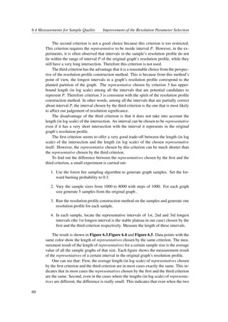
To understand this phenomenon more clearly, I did a small experiment: I generated
a graph with 10,000 nodes with configurations as listed in Table 5.1 and I ran the forest
fire sampling algorithm on the original graph with a forward burning probability of 0.3.
I counted the number of intervals within the range of resolution parameters [0.5,1] (I
took the average value for the number of intervals). The result is shown in Figure 6.2.
The horizontal axis shows the size of the sample graphs and the vertical axis shows
the number of intervals within the range [0.5,1] of the resolution parameter. The figure
shows that as the size of the graph sample decreases, the number of intervals decreases,
which indicates that smaller intervals are merged into larger intervals.
Figure 6.2: Number Of Intervals(Forest Fire,p=0.3)
The resolution profile of a graph sample can be viewed as an estimation of the
resolution profile of the original graph. Therefore, for the phenomenon that the long
plateaus in the resolution profile of a sample graph do not match the stable plateau in
the resolution profile of the original graph, the guess of cause of this phenomenon can
be formulated from the perspective of estimation. By doing so the fourth hypothesis is
obtained, as follows:
Hypothesis 4: The cause of the mismatch of stable plateaus between the sample
graph’s resolution profile and the original graph’s resolution profile is that: the graph
samples have underestimated long intervals and overestimated short intervals in the
resolution profile of the original graph.
In this hypothesis, "overestimate" means that an interval in the original graph’s res-
olution profile is shorter (in log scale) than the corresponding interval in the sample’s
resolution profile.
6.4 Measurements for Sample Quality
This section presents the measurements that are used to quantify the behaviour of graph
sampling algorithms.
57](https://image.slidesharecdn.com/ec58efe6-1586-42e4-a835-6c94f500953f-151224220719/85/thesis-69-320.jpg)
![6.4 Measurements for Sample Quality Improvement of the Resolution Parameter Selection
6.4.1 Precision of Plateau Estimation
In order to verify the first three hypotheses, we need to define a measurement which
is able to show how much the resolution profile of the sample "agrees" with the res-
olution profile of the original graph. In the following it will be explained how this
measurement is devised:
The first idea is to look at the estimation of the significance of the graph samples.
The rationale is that the closer the significance values of the sample graph’s commu-
nities and the original graph’s communities, the more similar the resolution profiles
of the two graphs. However, it is suggested in[31] that for an Erd˝os-Rényi random
graph, the maximum value of significance that a partition can achieve in a graph scales
with graph size. The significance of communities of Erd˝os-Rényi random graphs scale
approximately as nlogn, where n is the number of nodes in the graph. Therefore, the
significance value of the original graph’s partition cannot be directly compared to the
significance value of the graph sample’s partition. A possible solution would be to
divide the significance value by the scaling factor nlogn, but for graphs which are not
Erd˝os-Rényi random graph, the scaling factor might not be nlogn. This indicates that
it is not a good idea to compare the significance of a partition of the original graph
with the significance of a partition of a sample of this graph.
The second idea is to look at the resolution profile directly. Since in the resolution
profile construction method, we only care about the intervals in the resolution profile
that are significantly longer than the others (stable plateaus), we do not need to com-
pare all the intervals. We only consider the longest intervals (the longer the interval,
the more clear-cut the community structure).
Based on this idea, the precision of stable plateaus is defined as follows: Suppose
the longest interval in the resolution profile of the original graph is S, the longest
interval in the resolution profile of this graph’s sample is S . The precision is the
length (in log scale) of the intersection between S and S divided by the length (in log
scale) of S .
Similarly, if the original graph shows a hierarchical structure, the precision for the
second longest interval, third longest interval...et cetera, could be defined in a similar
way.
For example, if the longest interval of the original graph is [0.2,0.5] and the longest
interval of the sample is [0.15,0.4], then the precision is log0.4−log0.2
log0.4−log0.15.
A disadvantage of the precision of plateau estimate is that it is very sensitive to
relative ordering of lengths (in log scale) of intervals in the resolution profile. Suppose
A is the actual stable plateau and B is an interval in the resolution profile of the sample
and B has a long intersection with A. If B is slightly shorter than the stable plateau C
in the resolution profile of this graph sample, the precision result could be very bad,
because in this case precision is calculated from the perspective of C.
Despite this disadvantage, the measurement of precision can still give us an idea
about how a sample algorithm performs. The measurement is reasonable, because
when we try to estimate stable plateaus in a graph’s resolution profile from this graph’s
sample, we do not have prior knowledge about this graph’s resolution profile. The
relative ordering of lengths of intervals does affect our judgement about the positions
of stable plateaus, so it is reasonable to reflect this in the measurement of precision.
In other words, precision is unstable because the process of estimating the resolution
58](https://image.slidesharecdn.com/ec58efe6-1586-42e4-a835-6c94f500953f-151224220719/85/thesis-70-320.jpg)


![6.5 Experiment Setup Improvement of the Resolution Parameter Selection
Range Log Length
(0.0078125,0.0441941738242) 0.75257498916
(0.800354433289,1.0) 0.0967176450914
(0.00185017185702,0.0020437432591) 0.0432142669554
(0.505102622537,0.551938001461) 0.0385106732733
(0.456025846352,0.489617341633) 0.0308673335394
Table 6.2: Top 5 Stable Plateau of the Graph
To avoid this problem, a possible approach is to use a measurement that considers
all intervals in the resolution profile. This is difficult, because comparing the similar-
ity of intervals is difficult. For example, can you tell how similar [0,0.5,0.6,1] and
[0,0.3,0.4,1] are? Besides, it is unnecessary to consider every interval in the whole
range of valid resolution parameters because not all intervals are equally important.
In the resolution profile construction method we only consider those intervals that are
significantly longer than other intervals. The second problem can be solved by taking
into account more subtle cases in the interpretation, but this drastically increases the
complexity of the measurement. Therefore in general, although there might be a better
measurement, measuring length (in log scale) of representative is already good enough
as the first step to solve the problem of understanding the behavior of a sampling algo-
rithm and its influence on the resolution profile of a graph.
Although we can measure the length (in log scale) of representatives as a first step,
we cannot turn a blind eye to these problems. We must be very cautious about the
experiment design and the interpretation of the experiment results.
6.5 Experiment Setup
This section presents the setting of the experiments. A graph with 10,000 nodes is
generated. The top five intervals (in terms of length in log scale) in the resolution
profile of this graph are shown in Table 6.2 and a visualization of the resolution profile
is shown in Figure 6.6.
In Figure 6.6, the horizontal axis shows the resolution parameters in log scale and
the vertical axis shows the total number of internal edges of the communities. One can
see from the figure that there is only one stable plateau. Therefore, we only calculate
the precision from the perspective of this stable plateau (the longest interval in the
original graph’s resolution profile, in log scale). In the following discussion, "the
stable plateau in the resolution profile" means "the longest interval in the resolution
profile".
In the following, when speaking of "the original graph", I mean this graph.
6.6 Measurement Results of the Forest Fire Sampling
Method
In this section we generate graph samples using the forest fire sampling strategy and
evaluate the precision of the stable plateau estimate of different sizes of graph samples.
64](https://image.slidesharecdn.com/ec58efe6-1586-42e4-a835-6c94f500953f-151224220719/85/thesis-76-320.jpg)


![6.10 Summary Improvement of the Resolution Parameter Selection
Oversimplified Interpretation
The definition of representative is based on the third criterion (described in section
6.4.2). It is possible that the interpretation of the notion of representative is over-
simplified and in fact more complicated things are taking place. For example, if two
intervals A and B share the same representative in the resolution profile of a sample,
can we simply say "this implies that these two intervals in the original graph’s reso-
lution profile are ’merged’ in the sample graph’s resolution profile"? This is in fact
questionable: it is likely that this representative has a very small intersection with both
A and B. In this case, the indication of "merging" is not valid.
However, as is discussed in section 6.4.2, in most cases the representative chosen
by the first criterion and the third criterion are the same. Even if there is a difference,
it is small. This indicates that even though the third criterion does not require the
intersection to be long, the representative chosen by the third criterion has a similar
length as the representative chosen by the first criterion. Therefore, this problem does
not have a significant influence on the comparison of the lengths of representatives.
Characteristics of the Resolution Profile of the Original Graph
Particular characteristics of the resolution profile may invalidate the hypotheses. For
example, intervals that are closer to 1 may be less "damaged" by the decrease of the
graph size. As a result, if the stable plateau is close to 1, for example (0.5,1), it is pos-
sible that the length of the representative of the stable plateau in the original graph’s
resolution profile continuously increases as the sample size decreases, instead of show-
ing a "U" shape.
Graph Configuration
The graph samples studied in this chapter are all generated from one graph. The dif-
ference in graph types and configurations is not taken into account in the experiments.
In fact, different graph configurations and different graph types may invalidate the
hypotheses.
First, if the graph is generated from the Erd˝os-Rényi model, it is possible that the
representative of the longest stable plateau behaves in a different way as sample size
decreases. It is also possible that you cannot find a clear pattern in the change of the
length (in log scale) of the representatives as sample size decreases.
Second, if I choose different values for the minimum and maximum community
size, the stable plateaus in the resolution profile of the graph may change. It is possible
that the length of their representatives may change in a different way as sample size
decreases, which invalidates the hypotheses for the length of representatives and the
precision of stable plateau estimation.
6.10 Summary
In this chapter the possibility to accelerate the resolution profile construction method
proposed in [31] by graph sampling was explored. First, four hypotheses about sam-
pling methods were proposed. Based on these hypotheses, two different metrics, pre-
cision and length (in log scale) of representative, were proposed in order to measure
84](https://image.slidesharecdn.com/ec58efe6-1586-42e4-a835-6c94f500953f-151224220719/85/thesis-96-320.jpg)


![7.2 Answer to Research Questions Conclusions and Future Work
The second contribution of this thesis is that the possibility to speedup the res-
olution parameter selection with graph sampling is explored. Two sampling strate-
gies, the forest fire sampling algorithms and the random node selection algorithm, are
compared. Hypotheses on the difference between these two sampling algorithms are
proposed and measurements to quantify the behavior of these sampling algorithms are
devised based on these hypotheses. In the experiments it seems that the forest fire
sampling algorithm with a forward burning probability of 0.6 is more likely to gener-
ate better graph samples when the sample size is small. However, when the number of
nodes of graph samples is less than 50% of the original graph, neither of the two sam-
pling strategies is able to give satisfactory results, even though the forest fire sampling
algorithm with a forward burning probability of 0.6 generates a slightly better result.
7.2 Answer to Research Questions
Question 1: How to distribute the execution of the Louvain community detection al-
gorithm using big data tools such as Apache Spark?
The original sequential Louvain community detection algorithm looks at nodes in
the graph one by one. Each node joins one of its neighbouring communities which
gives a maximum increase of modularity. If no positive increase of modularity is pos-
sible, the node will stay in its original community. This algorithm can be distributed
by introducing the idea of the gossip algorithm: in each iteration, all nodes make their
decisions to join one of their neighbouring communities or stay in its original com-
munity. Each node has a probability p to join the community that gives a maximum
increase of modularity locally and a probability 1− p to do nothing. We can implement
this synchronous algorithm using Apache Spark. We then have a distributed version of
the Louvain community detection algorithm.
Question 2: How is the performance of the distributed version in comparison with
original sequential Louvain method? What characteristics does the distributed version
shows in execution?
In terms of the quality of partitions generated, the Distributed Synchronous Lou-
vain algorithm is very similar to the original sequential Louvain algorithm. The Dis-
tributed Synchronous Louvain algorithm has some very interesting characteristics.
First, the update probability (the probability that a node will join the neighbouring
community or its own original community that gives the maximum increase of modu-
larity) influences the number of iterations for the algorithm to converge, but it does not
influence the quality of partitions generated. Second, for the LFR benchmark, when
the mixing parameter is less than 0.5 and all the other configurations are the same
(such as number of nodes, minimum and maximum communities sizes), the number of
iterations for the algorithm to converge is almost the same , no matter what the mixing
parameter is.
Question 3: To accelerate the resolution parameter selection of the CPM commu-
nity detection algorithm, one possibility is to take a sample of the graph and select
resolution parameters based on this sample. To do so, the sample graph should give
us a good estimation of the resolution profile of the original graph. Among the many
graph sampling strategies, which is the best one to use, so that the estimation of the
resolution profile[31] of the original graph is as good as possible?
88](https://image.slidesharecdn.com/ec58efe6-1586-42e4-a835-6c94f500953f-151224220719/85/thesis-100-320.jpg)

![7.4 Future work Conclusions and Future Work
For the study of using graph sampling to accelerate the resolution parameter selec-
tion of the CPM community detection method, the following things can be done in the
future:
1. For now the graph samples are generated from one single graph. Due to time
constraints for this master thesis project, no more graphs are included in the
experiments. To further verify the validity of hypotheses proposed in this thesis,
more graphs of different types need to be studied in the future.
2. As is suggested in [31], the resolution profile of the Erd˝os-Rényi random graph
has a special characteristic: the density of the graph corresponds to the transition
point in the resolution profile (the place where the curve of N/n2 flattens. Here
n is the number of nodes and N is the sum of squares of community sizes). It
would be interesting to study the influence of graph sampling strategies to the
resolution profile of samples of Erd˝os-Rényi random graph.
90](https://image.slidesharecdn.com/ec58efe6-1586-42e4-a835-6c94f500953f-151224220719/85/thesis-102-320.jpg)
![Bibliography
[1] Lada A Adamic, Rajan M Lukose, Amit R Puniyani, and Bernardo A Huberman.
Search in power-law networks. Physical review E, 64(4):046135, 2001.
[2] Nesreen K Ahmed, Jennifer Neville, and Ramana Kompella. Network sampling:
From static to streaming graphs. arXiv preprint arXiv:1211.3412, 2012.
[3] Albert-László Barabási and Réka Albert. Emergence of scaling in random net-
works. science, 286(5439):509–512, 1999.
[4] Ginestra Bianconi and A-L Barabási. Competition and multiscaling in evolving
networks. EPL (Europhysics Letters), 54(4):436, 2001.
[5] Vincent D Blondel, Jean-Loup Guillaume, Renaud Lambiotte, and Etienne
Lefebvre. Fast unfolding of communities in large networks. Journal of Statistical
Mechanics: Theory and Experiment, 2008(10):P10008, 2008.
[6] Cumulative Advantage Distribution CAD. A generai theory of bibiiometric and
other cumulative advantage processes. Journal of the American society for Infor-
mation science, page 293, 1976.
[7] Leon Danon, Albert Diaz-Guilera, Jordi Duch, and Alex Arenas. Comparing
community structure identification. Journal of Statistical Mechanics: Theory
and Experiment, 2005(09):P09008, 2005.
[8] J-C Delvenne, Sophia N Yaliraki, and Mauricio Barahona. Stability of graph
communities across time scales. Proceedings of the National Academy of Sci-
ences, 107(29):12755–12760, 2010.
[9] Jordi Duch and Alex Arenas. Community detection in complex networks using
extremal optimization. Physical review E, 72(2):027104, 2005.
[10] Santo Fortunato. Community detection in graphs. Physics Reports, 486(3):75–
174, 2010.
[11] Santo Fortunato and Marc Barthélemy. Resolution limit in community detection.
Proceedings of the National Academy of Sciences, 104(1):36–41, 2007.
91](https://image.slidesharecdn.com/ec58efe6-1586-42e4-a835-6c94f500953f-151224220719/85/thesis-103-320.jpg)
![BIBLIOGRAPHY BIBLIOGRAPHY
[12] Michelle Girvan and Mark EJ Newman. Community structure in social and bio-
logical networks. Proceedings of the national academy of sciences, 99(12):7821–
7826, 2002.
[13] Roger Guimera, Stefano Mossa, Adrian Turtschi, and LA Nunes Amaral. The
worldwide air transportation network: Anomalous centrality, community struc-
ture, and cities’ global roles. Proceedings of the National Academy of Sciences,
102(22):7794–7799, 2005.
[14] Roger Guimera, Marta Sales-Pardo, and Luís A Nunes Amaral. Modularity
from fluctuations in random graphs and complex networks. Physical Review
E, 70(2):025101, 2004.
[15] Hawoong Jeong, Bálint Tombor, Réka Albert, Zoltan N Oltvai, and A-L
Barabási. The large-scale organization of metabolic networks. Nature,
407(6804):651–654, 2000.
[16] Andrea Lancichinetti and Santo Fortunato. Benchmarks for testing community
detection algorithms on directed and weighted graphs with overlapping commu-
nities. Physical Review E, 80(1):016118, 2009.
[17] Andrea Lancichinetti and Santo Fortunato. Consensus clustering in complex net-
works. Scientific reports, 2, 2012.
[18] Andrea Lancichinetti, Santo Fortunato, and Filippo Radicchi. Benchmark graphs
for testing community detection algorithms. Physical review E, 78(4):046110,
2008.
[19] Jure Leskovec and Christos Faloutsos. Sampling from large graphs. In Proceed-
ings of the 12th ACM SIGKDD international conference on Knowledge discovery
and data mining, pages 631–636. ACM, 2006.
[20] Atieh Mirshahvalad, Olivier H Beauchesne, Eric Archambault, and Martin Ros-
vall. Resampling effects on significance analysis of network clustering and rank-
ing. PloS one, 8(1):e53943, 2013.
[21] Atieh Mirshahvalad, Johan Lindholm, Mattias Derlen, and Martin Rosvall. Sig-
nificant communities in large sparse networks. PloS one, 7(3):e33721, 2012.
[22] Mark EJ Newman. Analysis of weighted networks. Physical Review E,
70(5):056131, 2004.
[23] Mark EJ Newman and Michelle Girvan. Finding and evaluating community
structure in networks. Physical review E, 69(2):026113, 2004.
[24] Arnau Prat-Pérez, David Dominguez-Sal, and Josep-LLuis Larriba-Pey. High
quality, scalable and parallel community detection for large real graphs. In Pro-
ceedings of the 23rd international conference on World wide web, pages 225–
236. ACM, 2014.
[25] Jörg Reichardt and Stefan Bornholdt. Partitioning and modularity of graphs with
arbitrary degree distribution. Physical Review E, 76(1):015102, 2007.
92](https://image.slidesharecdn.com/ec58efe6-1586-42e4-a835-6c94f500953f-151224220719/85/thesis-104-320.jpg)
![BIBLIOGRAPHY BIBLIOGRAPHY
[26] Bruno Ribeiro and Don Towsley. Estimating and sampling graphs with multidi-
mensional random walks. In Proceedings of the 10th ACM SIGCOMM confer-
ence on Internet measurement, pages 390–403. ACM, 2010.
[27] Peter Ronhovde and Zohar Nussinov. Multiresolution community detection for
megascale networks by information-based replica correlations. Physical Review
E, 80(1):016109, 2009.
[28] Satu Elisa Schaeffer. Graph clustering. Computer Science Review, 1(1):27–64,
2007.
[29] ChengTe Li ShouDe Lin, MiYen Yeh. Sampling and Summarization for Social
Networks. http://www.siam.org/meetings/sdm13/lin.pdf, 2013. [SDM
2013 Tutorial].
[30] VA Traag. Faster unfolding of communities: speeding up the louvain algorithm.
arXiv preprint arXiv:1503.01322, 2015.
[31] Vincent A Traag, Gautier Krings, and Paul Van Dooren. Significant scales in
community structure. Scientific reports, 3, 2013.
[32] Vincent A Traag, Paul Van Dooren, and Yurii Nesterov. Narrow scope for
resolution-limit-free community detection. Physical Review E, 84(1):016114,
2011.
[33] James M Varah. A lower bound for the smallest singular value of a matrix. Linear
Algebra and its Applications, 11(1):3–5, 1975.
93](https://image.slidesharecdn.com/ec58efe6-1586-42e4-a835-6c94f500953f-151224220719/85/thesis-105-320.jpg)