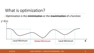
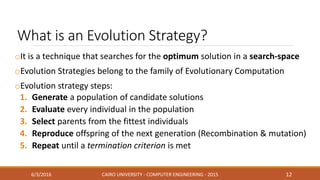
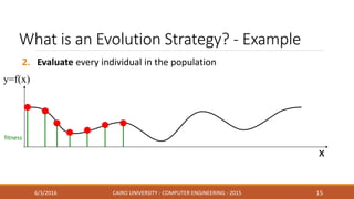
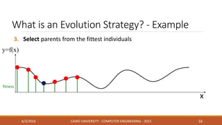
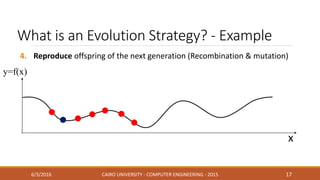
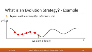
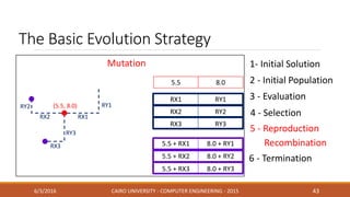
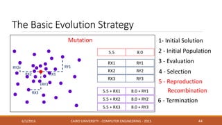
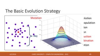
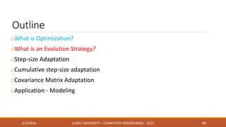
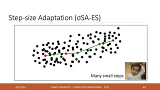
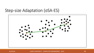
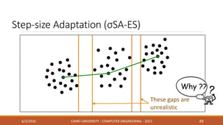
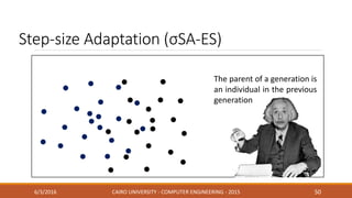
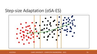
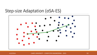
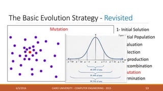
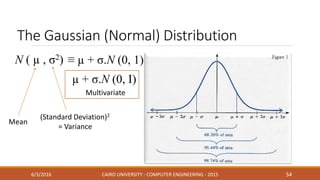
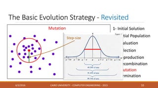
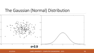
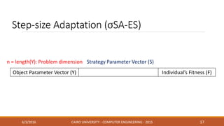
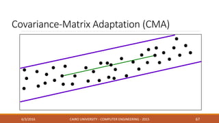
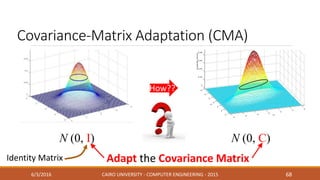
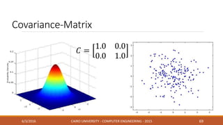
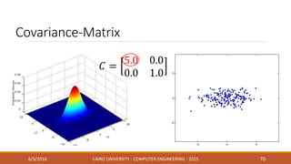
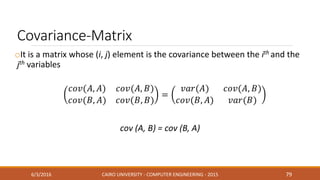
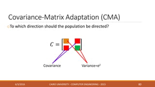
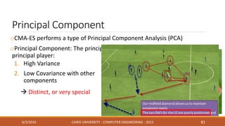
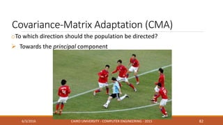
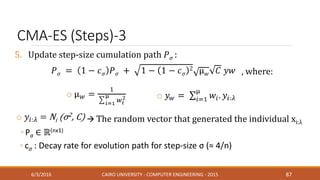
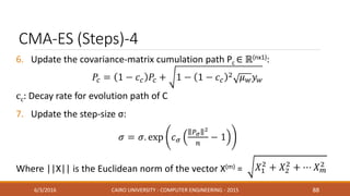
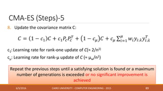
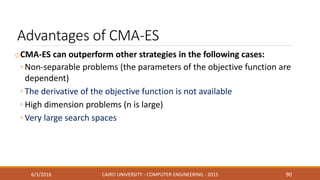
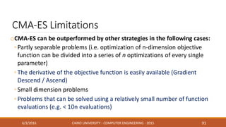
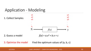
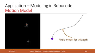
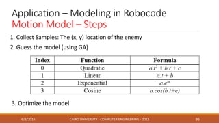
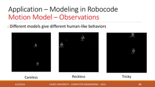
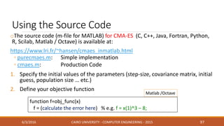
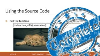
This document discusses covariance matrix adaptation evolution strategy (CMA-ES), an optimization technique. It begins with an introduction to optimization and evolution strategies. CMA-ES adapts the covariance matrix of a multivariate normal distribution used to sample new solutions, allowing it to better model the objective function. The document covers step-size adaptation, cumulative step-size adaptation, and covariance matrix adaptation, with examples provided.

1. Covariance Matrix Adaptation Evolution
Strategy (CMA-ES)
BY:
OSAMA SALAH ELDIN
UNDER SUPERVISION:
PROF. MAGDA B. FAYEK
6/3/2016 CAIRO UNIVERSITY - COMPUTER ENGINEERING - 2015

2. Outline
oWhat is Optimization?
oWhat is an Evolution Strategy?
oStep-size Adaptation
oCumulative step-size adaptation
oCovariance Matrix Adaptation
oApplication - Modeling
6/3/2016 CAIRO UNIVERSITY - COMPUTER ENGINEERING - 2015 2

3. What is optimization?
oOptimization is the minimization or the maximization of a function
6/3/2016 CAIRO UNIVERSITY - COMPUTER ENGINEERING - 2015 3
y=f(x)
Global MinimumLocal Minimum xLocal Minimum

4. What is optimization?
oTry to solve these problems:
6/3/2016 CAIRO UNIVERSITY - COMPUTER ENGINEERING - 2015 4
x = 2
x3 – 8 = 0

5. What is optimization?
oTry to solve these problems:
6/3/2016 CAIRO UNIVERSITY - COMPUTER ENGINEERING - 2015 5
x=3, y=2
x2 + 3.y – 15 = 0

6. What is optimization?
oTry to solve these problems:
6/3/2016 CAIRO UNIVERSITY - COMPUTER ENGINEERING - 2015 6
x=3, y=2, z=2
x2 + y + 2.z – 15 = 0

7. What is optimization?
oTry to solve these problems:
6/3/2016 CAIRO UNIVERSITY - COMPUTER ENGINEERING - 2015 7

8. What is optimization?
oTry to solve these problems:
6/3/2016 CAIRO UNIVERSITY - COMPUTER ENGINEERING - 2015 8
Can one try all combinations??
This is not recommended

9. What is optimization?
6/3/2016 CAIRO UNIVERSITY - COMPUTER ENGINEERING - 2015 9
Use an evolution strategy

10. Outline
oWhat is Optimization?
oWhat is an Evolution Strategy?
oStep-size Adaptation
oCumulative step-size adaptation
oCovariance Matrix Adaptation
oApplication - Modeling
6/3/2016 CAIRO UNIVERSITY - COMPUTER ENGINEERING - 2015 10

11. 6/3/2016 CAIRO UNIVERSITY - COMPUTER ENGINEERING - 2015 11
What is an Evolution Strategy?

12. What is an Evolution Strategy?
oIt is a technique that searches for the optimum solution in a search-space
oEvolution Strategies belong to the family of Evolutionary Computation
oEvolution strategy steps:
1. Generate a population of candidate solutions
2. Evaluate every individual in the population
3. Select parents from the fittest individuals
4. Reproduce offspring of the next generation (Recombination & mutation)
5. Repeat until a termination criterion is met
6/3/2016 CAIRO UNIVERSITY - COMPUTER ENGINEERING - 2015 12

13. Evolution Strategies VS. Genetic Algorithms
ES GA
Initial Population
Random mutations of the
initial guess
Random or seeded
Evaluation Objective Function Fitness (Evaluation) Function
Selection Truncation Selection Different methods
Reproduction Recombination + Mutation Crossover + Mutation
Termination Almost similar stop conditions
6/3/2016 CAIRO UNIVERSITY - COMPUTER ENGINEERING - 2015 13

14. What is an Evolution Strategy? - Example
1. Generate a population of candidate solutions
6/3/2016 CAIRO UNIVERSITY - COMPUTER ENGINEERING - 2015 14
y=f(x)
x

15. fitness
What is an Evolution Strategy? - Example
2. Evaluate every individual in the population
6/3/2016 CAIRO UNIVERSITY - COMPUTER ENGINEERING - 2015 15
y=f(x)
x

16. fitness
What is an Evolution Strategy? - Example
3. Select parents from the fittest individuals
6/3/2016 CAIRO UNIVERSITY - COMPUTER ENGINEERING - 2015 16
y=f(x)
x

17. What is an Evolution Strategy? - Example
4. Reproduce offspring of the next generation (Recombination & mutation)
6/3/2016 CAIRO UNIVERSITY - COMPUTER ENGINEERING - 2015 17
y=f(x)
x

18. What is an Evolution Strategy? - Example
5. Repeat until a termination criterion is met
6/3/2016 CAIRO UNIVERSITY - COMPUTER ENGINEERING - 2015 18
y=f(x)
xEvaluate & Select

19. What is an Evolution Strategy? - Example
5. Repeat until a termination criterion is met
6/3/2016 CAIRO UNIVERSITY - COMPUTER ENGINEERING - 2015 19
y=f(x)
xEvaluate & SelectReproduce

20. What is an Evolution Strategy? - Example
5. Repeat until a termination criterion is met
6/3/2016 CAIRO UNIVERSITY - COMPUTER ENGINEERING - 2015 20
y=f(x)
x
Optimum Solution
Evaluate – Select – ReproduceReproduceTerminate

21. The Basic Evolution Strategy
oThe basic evolution strategy is defined by:
(µ/ρ, λ)-ES and (µ/ρ+ λ)-ES
Where:
µ The number of selected individuals per generation
ρ The number of parents (selected from µ) involved in recombination (≤ µ)
λ The number of individuals per generation (population size)
, Comma Selection  µ parents are selected from the λ individuals
+ Plus Selection  µ parents are selected from the λ individuals + the
current ρ parents
6/3/2016 CAIRO UNIVERSITY - COMPUTER ENGINEERING - 2015 21

22. The Basic Evolution Strategy - Example
(10/6 , 50)-ES
Select the fittest 10 individuals from the 50 individuals of the current
population, and select 6 random ones from them. Recombine these 6
parents to generate 50 new offspring
(10/6 + 50)-ES
Select the fittest 10 individuals from the 50 individuals of the current
population along with their 6 parents, and select 6 random ones from them
all (from the 56). Recombine these 6 parents to generate 50 new offspring
6/3/2016 CAIRO UNIVERSITY - COMPUTER ENGINEERING - 2015 22

23. The structure of an Individual
Object Parameter Vector (Y) Strategy Parameter Vector (S) Individual’s Fitness (F)
6/3/2016 CAIRO UNIVERSITY - COMPUTER ENGINEERING - 2015 23
Y The candidate solution of the problem (e.g. (x, y) point)
S The parameters used by the strategy (e.g. mutation strength)
F The fitness of the candidate solution y as measured by the fitness
function (i.e. the value of the objective function)
Y = {x1, x2, z}

24. The structure of an Individual
Object Parameter Vector (Y) Strategy Parameter Vector (S) Individual’s Fitness (F)
6/3/2016 CAIRO UNIVERSITY - COMPUTER ENGINEERING - 2015 24
• Evolution strategies search for the optimum:
1. Solution: The highest fitness
2. Strategy Parameters: The fastest improvement
Two search spaces

25. ES Steps
6/3/2016 CAIRO UNIVERSITY - COMPUTER ENGINEERING - 2015 25
1- Initial Solution

26. 2 - Initial Population
ES Steps
6/3/2016 CAIRO UNIVERSITY - COMPUTER ENGINEERING - 2015 26
1- Initial Solution

27. 2 - Initial Population
ES Steps
6/3/2016 CAIRO UNIVERSITY - COMPUTER ENGINEERING - 2015 27
3 - Evaluation 1- Initial Solution

28. 3 - Evaluation4 - Selection
ES Steps
6/3/2016 CAIRO UNIVERSITY - COMPUTER ENGINEERING - 2015 28
µ = 4 ρ=1 2 - Initial Population
1- Initial Solution

29. 5 - Reproduction
ES Steps
6/3/2016 CAIRO UNIVERSITY - COMPUTER ENGINEERING - 2015 29
2 - Initial Population
1- Initial Solution
3 - Evaluation
4 - Selection

30. 5 - Reproduction
ES Steps
6/3/2016 CAIRO UNIVERSITY - COMPUTER ENGINEERING - 2015 30
2 - Initial Population
1- Initial Solution
3 - Evaluation
4 - Selection

31. ES Steps
6/3/2016 CAIRO UNIVERSITY - COMPUTER ENGINEERING - 2015 31
2 - Initial Population
1- Initial Solution
3 - Evaluation
4 - Selection
5 - Reproduction

32. ES Steps
6/3/2016 CAIRO UNIVERSITY - COMPUTER ENGINEERING - 2015 32
2 - Initial Population
1- Initial Solution
3 - Evaluation
4 - Selection
5 - Reproduction

33. 6 - Termination
ES Steps
6/3/2016 CAIRO UNIVERSITY - COMPUTER ENGINEERING - 2015 33
2 - Initial Population
1- Initial Solution
3 - Evaluation
4 - Selection
Optimum Solution
5 - Reproduction

34. The Basic Evolution Strategy
6/3/2016 CAIRO UNIVERSITY - COMPUTER ENGINEERING - 2015 34
2 - Initial Population
1- Initial Solution
3 - Evaluation
4 - Selection
• An initial guess, should be as close as possible to
the expected solution
6 - Termination
5 - Reproduction

35. The Basic Evolution Strategy
6/3/2016 CAIRO UNIVERSITY - COMPUTER ENGINEERING - 2015 35
2 - Initial Population
1- Initial Solution
3 - Evaluation
4 - Selection
• The intial population is generated by mutating the
initial solution
6 - Termination
5 - Reproduction

36. The Basic Evolution Strategy
6/3/2016 CAIRO UNIVERSITY - COMPUTER ENGINEERING - 2015 36
2 - Initial Population
1- Initial Solution
3 - Evaluation
4 - Selection
• Every individual is evaluated by the objective
function
6 - TerminationBest Fitness = 0
5 - Reproduction

37. The Basic Evolution Strategy
6/3/2016 CAIRO UNIVERSITY - COMPUTER ENGINEERING - 2015 37
2 - Initial Population
1- Initial Solution
3 - Evaluation
4 - Selection
• Truncation Selection is used
6 - Termination
5 - Reproduction
Select the fittest µ individuals
Drop the other individuals

38. The Basic Evolution Strategy
6/3/2016 CAIRO UNIVERSITY - COMPUTER ENGINEERING - 2015 38
2 - Initial Population
1- Initial Solution
3 - Evaluation
4 - Selection
5 - Reproduction
6 - Termination
Recombination
Reproduction
Mutation
Combining two or more
parents to produce a mean
for the new generation
Adding normally-
distributed random vectors
to the new mean

39. The Basic Evolution Strategy
6/3/2016 CAIRO UNIVERSITY - COMPUTER ENGINEERING - 2015 39
2 - Initial Population
1- Initial Solution
3 - Evaluation
4 - Selection
5 - Reproduction
6 - Termination
Recombination
S1 F11 3
S2 F24 6
Solution Strategy Parameters
S32.5 4.5
A simple recombination is taking the average
P1
P2
Fitness
To be calculated

40. The Basic Evolution Strategy
6/3/2016 CAIRO UNIVERSITY - COMPUTER ENGINEERING - 2015 40
2 - Initial Population
1- Initial Solution
3 - Evaluation
4 - Selection
5 - Reproduction
6 - Termination
Recombination
ρ = 2 ρ = 4

41. The Basic Evolution Strategy
6/3/2016 CAIRO UNIVERSITY - COMPUTER ENGINEERING - 2015 41
2 - Initial Population
1- Initial Solution
3 - Evaluation
4 - Selection
5 - Reproduction
6 - Termination
Recombination Mutation
Reproduction
Combining two or more
parents to produce a mean
for the new generation
Adding normally-
distributed random vectors
to the new mean

42. The Basic Evolution Strategy
6/3/2016 CAIRO UNIVERSITY - COMPUTER ENGINEERING - 2015 42
2 - Initial Population
1- Initial Solution
3 - Evaluation
4 - Selection
5.5 8.0Parent
RX1 RY1
Generate λ normally-distributed
random vectors
RX2 RY2
RX3 RY3
5.5 + RX1 8.0 + RY1
5.5 + RX2 8.0 + RY2
5.5 + RX3 8.0 + RY3
Add each of the λ mutating vectors
to the initial solution 6 - Termination
5 - Reproduction
Mutation
Recombination

43. The Basic Evolution Strategy
6/3/2016 CAIRO UNIVERSITY - COMPUTER ENGINEERING - 2015 43
2 - Initial Population
1- Initial Solution
3 - Evaluation
4 - Selection
5.5 8.0
RX1 RY1
RX2 RY2
RX3 RY3
RX1
RY1
5.5 + RX1 8.0 + RY1
5.5 + RX2 8.0 + RY2
5.5 + RX3 8.0 + RY3
RX2
RY2
RX3
RY3
5 - Reproduction
Mutation
6 - Termination
Recombination
(5.5, 8.0)

44. The Basic Evolution Strategy
6/3/2016 CAIRO UNIVERSITY - COMPUTER ENGINEERING - 2015 44
2 - Initial Population
1- Initial Solution
3 - Evaluation
4 - Selection
5.5 8.0
RX1 RY1
RX2 RY2
RX3 RY3
5.5 + RX1 8.0 + RY1
5.5 + RX2 8.0 + RY2
5.5 + RX3 8.0 + RY3
RX1
RY1
RX2
RY2
RX3
RY3
5 - Reproduction
6 - Termination
Recombination
Mutation

45. 6 - Termination
Mutation vectors are
normally – distributed
around their parent
Recombination
5 - Reproduction
The Basic Evolution Strategy
6/3/2016 CAIRO UNIVERSITY - COMPUTER ENGINEERING - 2015 45
2 - Initial Population
1- Initial Solution
3 - Evaluation
4 - Selection
Repeat
Mutation

46. Outline
oWhat is Optimization?
oWhat is an Evolution Strategy?
oStep-size Adaptation
oCumulative step-size adaptation
oCovariance Matrix Adaptation
oApplication - Modeling
6/3/2016 CAIRO UNIVERSITY - COMPUTER ENGINEERING - 2015 46

47. Step-size Adaptation (σSA-ES)
6/3/2016 CAIRO UNIVERSITY - COMPUTER ENGINEERING - 2015 47
Many small steps

48. Step-size Adaptation (σSA-ES)
6/3/2016 CAIRO UNIVERSITY - COMPUTER ENGINEERING - 2015 48

49. Step-size Adaptation (σSA-ES)
6/3/2016 CAIRO UNIVERSITY - COMPUTER ENGINEERING - 2015 49
These gaps are
unrealistic
Why ??

50. Step-size Adaptation (σSA-ES)
6/3/2016 CAIRO UNIVERSITY - COMPUTER ENGINEERING - 2015 50
The parent of a generation is
an individual in the previous
generation

51. Step-size Adaptation (σSA-ES)
6/3/2016 CAIRO UNIVERSITY - COMPUTER ENGINEERING - 2015 51

52. Step-size Adaptation (σSA-ES)
6/3/2016 CAIRO UNIVERSITY - COMPUTER ENGINEERING - 2015 52

53. 6 - Termination
Recombination
5 - Reproduction
The Basic Evolution Strategy - Revisited
6/3/2016 CAIRO UNIVERSITY - COMPUTER ENGINEERING - 2015 53
2 - Initial Population
1- Initial Solution
3 - Evaluation
4 - Selection
Mutation
Mutation

54. The Gaussian (Normal) Distribution
6/3/2016 CAIRO UNIVERSITY - COMPUTER ENGINEERING - 2015 54
N ( µ , σ2)
Mean
(Standard Deviation)2
= Variance
≡ µ + σ.N (0, 1)
µ + σ.N (0, I)
Multivariate

55. 6 - Termination
Recombination
5 - Reproduction
The Basic Evolution Strategy - Revisited
6/3/2016 CAIRO UNIVERSITY - COMPUTER ENGINEERING - 2015 55
2 - Initial Population
1- Initial Solution
3 - Evaluation
4 - Selection
Mutation
Mutation
Step-size

56. The Gaussian (Normal) Distribution
6/3/2016 CAIRO UNIVERSITY - COMPUTER ENGINEERING - 2015 56
σ=1.0σ=1.5σ=2.0σ=2.5

57. Step-size Adaptation (σSA-ES)
6/3/2016 CAIRO UNIVERSITY - COMPUTER ENGINEERING - 2015 57
Object Parameter Vector (Y) Individual’s Fitness (F)
Strategy Parameter Vector (S)
σ
n = length(Y): Problem dimension

58. Outline
oWhat is Optimization?
oWhat is an Evolution Strategy?
oStep-size Adaptation
oCumulative step-size adaptation
oCovariance Matrix Adaptation
oApplication - Modeling
6/3/2016 CAIRO UNIVERSITY - COMPUTER ENGINEERING - 2015 58

59. Cumulative Step-size Adaptation (CSA)
oStep-size Adaptation
6/3/2016 CAIRO UNIVERSITY - COMPUTER ENGINEERING - 2015 59
Increase step size Decrease step size

60. Cumulative Step-size Adaptation (CSA)
6/3/2016 CAIRO UNIVERSITY - COMPUTER ENGINEERING - 2015 60
1. Calculate the average 𝑍𝑡 of the fittest µ solutions
2. Calculate the cumulative path Pc at generation t
The parameter c is called the cumulation parameter, it determines how rapidly
the information stored in Pct fades. The typical value of c is between 1/n and 1/

61. Cumulative Step-size Adaptation (CSA)
3. Update the mutation strength (i.e. step-size)
6/3/2016 CAIRO UNIVERSITY - COMPUTER ENGINEERING - 2015 61
The damping parameter dσ determines how much the step-size can
change. (Normally, it is set to 1)
Where ||𝑋||‖ is the Euclidean norm of the vector =

62. Cumulative Step-size Adaptation (CSA)
6/3/2016 CAIRO UNIVERSITY - COMPUTER ENGINEERING - 2015 62
Object Parameter Vector (Y) σ Individual’s Fitness (F)

63. Outline
oWhat is Optimization?
oWhat is an Evolution Strategy?
oStep-size Adaptation
oCumulative step-size adaptation
oCovariance Matrix Adaptation
oApplication - Modeling
6/3/2016 CAIRO UNIVERSITY - COMPUTER ENGINEERING - 2015 63

64. Promising
individuals
Covariance-Matrix Adaptation (CMA)
6/3/2016 CAIRO UNIVERSITY - COMPUTER ENGINEERING - 2015 64

65. Covariance-Matrix Adaptation (CMA)
6/3/2016 CAIRO UNIVERSITY - COMPUTER ENGINEERING - 2015 65

66. Covariance-Matrix Adaptation (CMA)
6/3/2016 CAIRO UNIVERSITY - COMPUTER ENGINEERING - 2015 66

67. Covariance-Matrix Adaptation (CMA)
6/3/2016 CAIRO UNIVERSITY - COMPUTER ENGINEERING - 2015 67

68. Covariance-Matrix Adaptation (CMA)
6/3/2016 CAIRO UNIVERSITY - COMPUTER ENGINEERING - 2015 68
N (0, I) N (0, C)
How??
Adapt the Covariance MatrixIdentity Matrix

69. Covariance-Matrix
6/3/2016 CAIRO UNIVERSITY - COMPUTER ENGINEERING - 2015 69

70. Covariance-Matrix
6/3/2016 CAIRO UNIVERSITY - COMPUTER ENGINEERING - 2015 70

71. Covariance-Matrix
6/3/2016 CAIRO UNIVERSITY - COMPUTER ENGINEERING - 2015 71

72. Covariance-Matrix
6/3/2016 CAIRO UNIVERSITY - COMPUTER ENGINEERING - 2015 72

73. Covariance-Matrix
6/3/2016 CAIRO UNIVERSITY - COMPUTER ENGINEERING - 2015 73

74. Covariance-Matrix Adaptation (CMA)
oTo which direction should the population be directed?
6/3/2016 CAIRO UNIVERSITY - COMPUTER ENGINEERING - 2015 74
VarianceCovariance

75. oVariance is a measure of how far a variable changes away from its mean
Variance
6/3/2016 CAIRO UNIVERSITY - COMPUTER ENGINEERING - 2015 75
, 𝑋 is the mean of the samples of X

76. 0
2
4
6
8
10
12
0
2
4
6
8
10
12
Variance
6/3/2016 CAIRO UNIVERSITY - COMPUTER ENGINEERING - 2015 76
High Variance
Low Variance
mean
mean

77. oCovariance is a measure of how two variables change together
Covariance
6/3/2016 CAIRO UNIVERSITY - COMPUTER ENGINEERING - 2015 77

78. Covariance
6/3/2016 CAIRO UNIVERSITY - COMPUTER ENGINEERING - 2015 78
(a)
(c)
Cov(a, c) = -3.0091
(b)
Cov(a, b) = 8.3909

79. Covariance-Matrix
oIt is a matrix whose (i, j) element is the covariance between the ith and the
jth variables
6/3/2016 CAIRO UNIVERSITY - COMPUTER ENGINEERING - 2015 79

80. Covariance-Matrix Adaptation (CMA)
oTo which direction should the population be directed?
6/3/2016 CAIRO UNIVERSITY - COMPUTER ENGINEERING - 2015 80
Variance=σ2Covariance

81. Principal Component
6/3/2016 CAIRO UNIVERSITY - COMPUTER ENGINEERING - 2015 81
oCMA-ES performs a type of Principal Component Analysis (PCA)
oPrincipal Component: The principal variable (component) is equivalent to the
principal player:
1. High Variance
2. Low Covariance with other
components
 Distinct, or very special

82. Covariance-Matrix Adaptation (CMA)
6/3/2016 CAIRO UNIVERSITY - COMPUTER ENGINEERING - 2015 82
oTo which direction should the population be directed?
 Towards the principal component

83. Covariance-Matrix Adaptation (CMA)
6/3/2016 CAIRO UNIVERSITY - COMPUTER ENGINEERING - 2015 83
• The optimum solution is (5, 50)
 A practical run of CMA-ES x
• The population moves faster
towards the direction of the
second component (50)
• The initial guess is (0, 0)

84. Covariance-Matrix Adaptation (CMA)
6/3/2016 CAIRO UNIVERSITY - COMPUTER ENGINEERING - 2015 84
optimum (5, 50)
Initial (0, 0)
generation
Variance
(σ2)
Step-size

85. CMA-ES (Steps)-1
oInitial Values
◦ C = I (n x n Identity Matrix)
◦ An initial guess m (n x 1 mean of the initial population)
◦ An initial step size (n x 1 standard-deviation matrix)
1. Generate λ offspring by mutating the mean m:
2. Evaluate the λ offspring
3. Sort the offspring by fitness so that:
6/3/2016 CAIRO UNIVERSITY - COMPUTER ENGINEERING - 2015 85
Fittest Individual

86. CMA-ES (Steps)-2
4. Update the mean m of the population
6/3/2016 CAIRO UNIVERSITY - COMPUTER ENGINEERING - 2015 86
 Weighted average
The constants wi are selected such that:
µ is the number of parents

87. CMA-ES (Steps)-3
5. Update step-size cumulation path 𝑃 𝜎 :
, where:
 The random vector that generated the individual xi:λ
◦ cσ : Decay rate for evolution path for step-size σ (≈ 4/n)
6/3/2016 CAIRO UNIVERSITY - COMPUTER ENGINEERING - 2015 87

88. CMA-ES (Steps)-4
6. Update the covariance-matrix cumulation path Pc ∈ ℝ(nx1):
cc: Decay rate for evolution path of C
7. Update the step-size σ:
Where ||X|| is the Euclidean norm of the vector X(m) =
6/3/2016 CAIRO UNIVERSITY - COMPUTER ENGINEERING - 2015 88

89. CMA-ES (Steps)-5
8. Update the covariance matrix C:
c1: Learning rate for rank-one update of C(≈ 2/n2)
cµ: Learning rate for rank-µ update of C (≈ µw/n2)
6/3/2016 CAIRO UNIVERSITY - COMPUTER ENGINEERING - 2015 89
Repeat the previous steps until a satisfying solution is found or a maximum
number of generations is exceeded or no significant improvement is
achieved

90. Advantages of CMA-ES
oCMA-ES can outperform other strategies in the following cases:
◦ Non-separable problems (the parameters of the objective function are
dependent)
◦ The derivative of the objective function is not available
◦ High dimension problems (n is large)
◦ Very large search spaces
6/3/2016 CAIRO UNIVERSITY - COMPUTER ENGINEERING - 2015 90

91. CMA-ES Limitations
oCMA-ES can be outperformed by other strategies in the following cases:
◦ Partly separable problems (i.e. optimization of n-dimension objective
function can be divided into a series of n optimizations of every single
parameter)
◦ The derivative of the objective function is easily available (Gradient
Descend / Ascend)
◦ Small dimension problems
◦ Problems that can be solved using a relatively small number of function
evaluations (e.g. < 10n evaluations)
6/3/2016 CAIRO UNIVERSITY - COMPUTER ENGINEERING - 2015 91

92. Outline
oWhat is Optimization?
oWhat is an Evolution Strategy?
oStep-size Adaptation
oCumulative step-size adaptation
oCovariance Matrix Adaptation
oApplication - Modeling
6/3/2016 CAIRO UNIVERSITY - COMPUTER ENGINEERING - 2015 92

93. Application - Modeling
6/3/2016 CAIRO UNIVERSITY - COMPUTER ENGINEERING - 2015 93
f(x)X y
2. Guess a model f(x) = a.x2 + b.x + c
1. Collect Samples
x1
x2
x3
.
.
xn
y1
y2
y3
.
.
yn
3. Optimize the model Find the optimum values of {a, b, c}

94. Application – Modeling in Robocode
Motion Model
6/3/2016 CAIRO UNIVERSITY - COMPUTER ENGINEERING - 2015 94
Find a model for this path

95. Application – Modeling in Robocode
Motion Model – Steps
1. Collect Samples: The (x, y) location of the enemy
2. Guess the model (using GA)
6/3/2016 CAIRO UNIVERSITY - COMPUTER ENGINEERING - 2015 95
3. Optimize the model

96. Application – Modeling in Robocode
Motion Model – Observations
oDifferent models give different human-like behaviors
6/3/2016 CAIRO UNIVERSITY - COMPUTER ENGINEERING - 2015 96
Careless Reckless Tricky

97. Using the Source Code
oThe source code (m-file for MATLAB) for CMA-ES (C, C++, Java, Fortran, Python,
R, Scilab, Matlab / Octave) is available at:
https://www.lri.fr/~hansen/cmaes_inmatlab.html
◦ purecmaes.m: Simple implementation
◦ cmaes.m: Production Code
1. Specify the initial values of the parameters (step-size, covariance matrix, initial
guess, population size … etc.)
2. Define your objective function
6/3/2016 CAIRO UNIVERSITY - COMPUTER ENGINEERING - 2015 97
function f=obj_func(x)
f = (calculate the error here) % e.g. f = x(1)^3 – 8;
Matlab /Octave

98. 3. Call the function Matlab /Octave
Using the Source Code
6/3/2016 CAIRO UNIVERSITY - COMPUTER ENGINEERING - 2015 98
>> function_mfile( parameters)

99. Questions
6/3/2016 CAIRO UNIVERSITY - COMPUTER ENGINEERING - 2015 99
osama.salah.eg@ieee.org

100. Thanks
6/3/2016 CAIRO UNIVERSITY - COMPUTER ENGINEERING - 2015 100