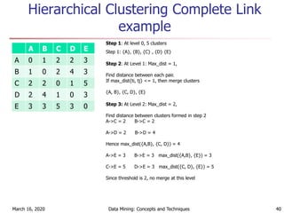
Download as PDF, PPTX

![K-means 2D example
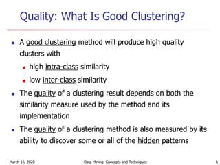
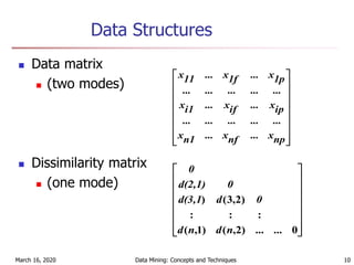
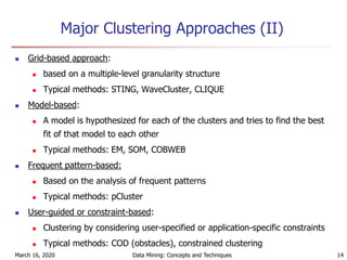
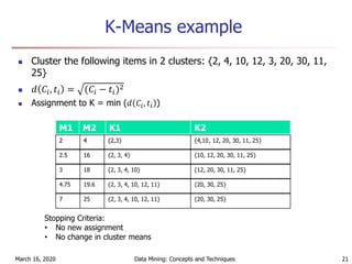
Apply k-means for the following dataset to make 2 clusters:
March 16, 2020 Data Mining: Concepts and Techniques 22
X Y
185 72
170 56
168 60
179 68
182 72
188 77
Step 1: Assume Initial Centroids: C1 = (185, 72), C2 = (170, 56)
Step 2: Calculate Euclidean Distance to each centroid:
𝑑[ 𝑥, 𝑦 , 𝑎, 𝑏 ] = (𝑥 − 𝑎)2+(𝑦 − 𝑏)2
For t1 = (168, 60)
𝑑[ 185,72 , 168, 60 ] = (185 − 168)2+(72 − 60)2
= 20.808
𝑑[ 170,56 , 168, 60 ] = (170 − 168)2+(56 − 60)2
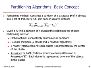
= 4.472
Since d(C2, t1) > d(C1,t1). So assign t1 to C2
Step 3: For t2 = (179, 68)
𝑑[ 185,72 , 179, 68 ] = (185 − 179)2+(72 − 68)2
= 7.211
𝑑[ 170,56 , 179, 68 ] = (170 − 179)2+(56 − 68)2
= 15
Since d(C1, t2) < d(C2,t2) So assign t2 to C1
Step 4: For t3 = (182, 72)
𝑑[ 185,72 , 182, 72 ] = (185 − 182)2+(72 − 72)2
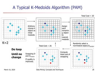
= 3
𝑑[ 170,56 , 182, 72 ] = (170 − 182)2+(56 − 72)2
= 20
Since d(C1, t3) < d(C2,t3), So assign t3 to C1](https://image.slidesharecdn.com/clustering-200316044218/85/Clustering-22-320.jpg)
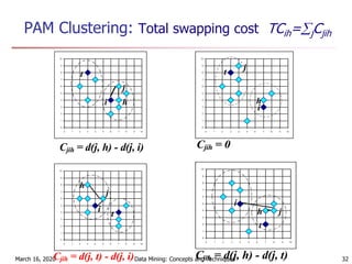
![K-means 2D example
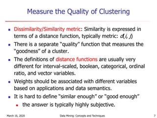
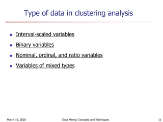
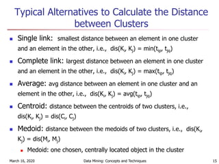
Apply k-means for the following dataset to make 2 clusters:
March 16, 2020 Data Mining: Concepts and Techniques 23
X Y
185 72
170 56
168 60
179 68
182 72
188 77
Step 5: For t4 = (188, 77)
𝑑[ 185,72 , 182, 72 ] = (185 − 188)2+(72 − 77)2
= 5.83
𝑑[ 170,56 , 182, 72 ] = (170 − 188)2+(56 − 77)2
= 27.65
Since d(C1, t4) < d(C2,t4), So assign t4 to C1
Step 6: Clusters after 1 iteration
D1 = {(185, 72), (179, 68), (182, 72), (188, 77)}
D2 = {(170, 56), (168, 60)}
Step 7: New clusters centroids C1 = {183.5, 72.25} C2 = {169, 116}
Repeat above steps for all samples till convergence
Final Clusters
D1 = {(185, 72), (179, 68), (182, 72), (188, 77)}
D2 = {(170, 56), (168, 60)}](https://image.slidesharecdn.com/clustering-200316044218/85/Clustering-23-320.jpg)
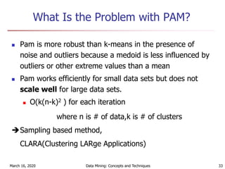
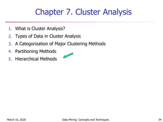
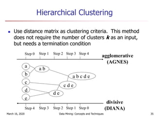
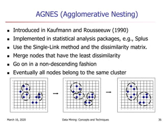

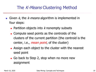
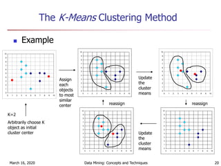
The document discusses cluster analysis and various clustering algorithms. It begins with an introduction to cluster analysis, describing what clusters are and some applications of clustering techniques. It then categorizes major clustering methods into partitioning methods, hierarchical methods, density-based methods, and others. Finally, it describes two partitioning algorithms - k-means and k-medoids - in more detail. The k-means algorithm is explained as selecting initial cluster centers, assigning all objects to the closest center, and updating centers repeatedly until convergence.