Download to read offline
![Statistical Model
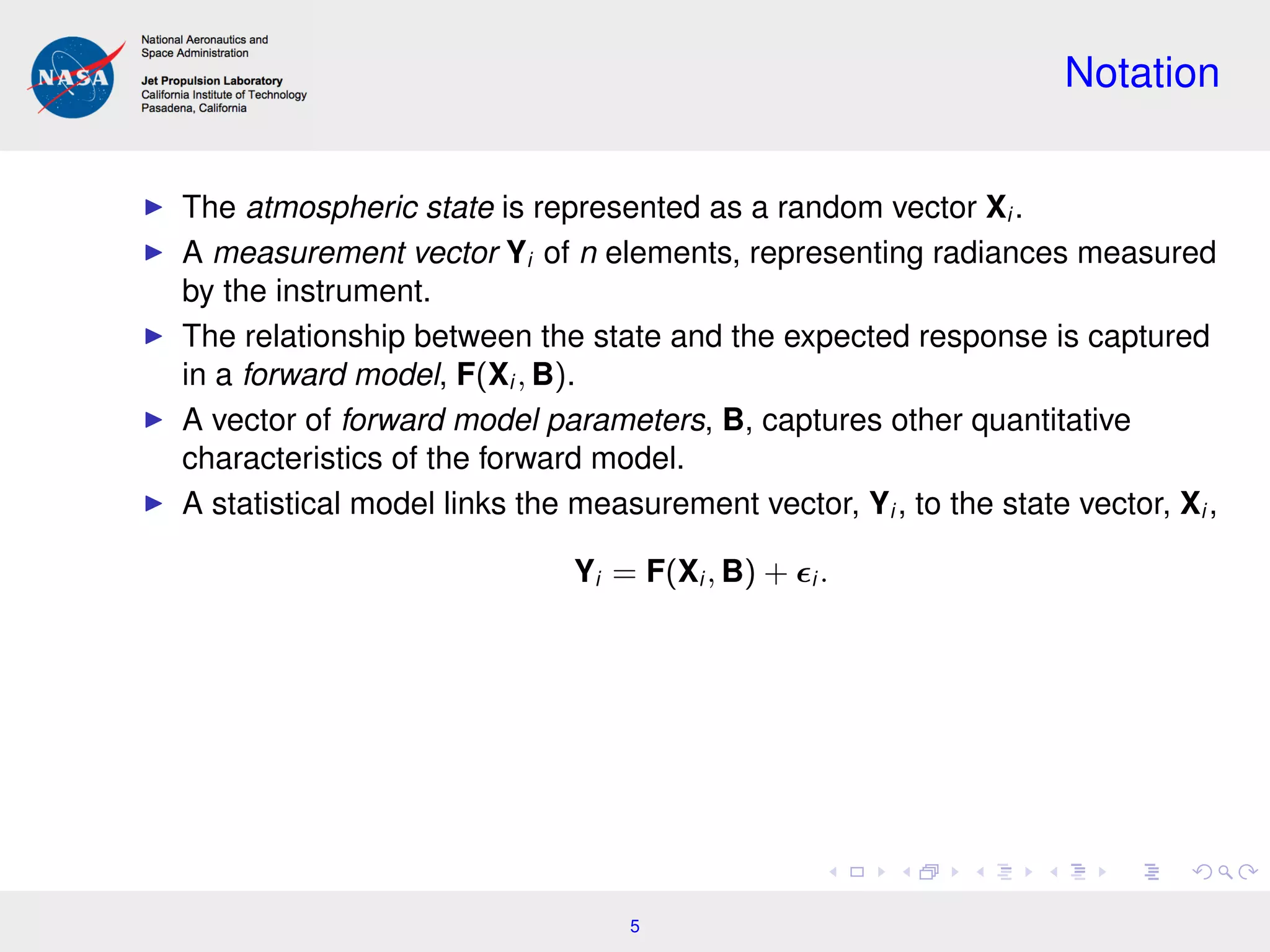
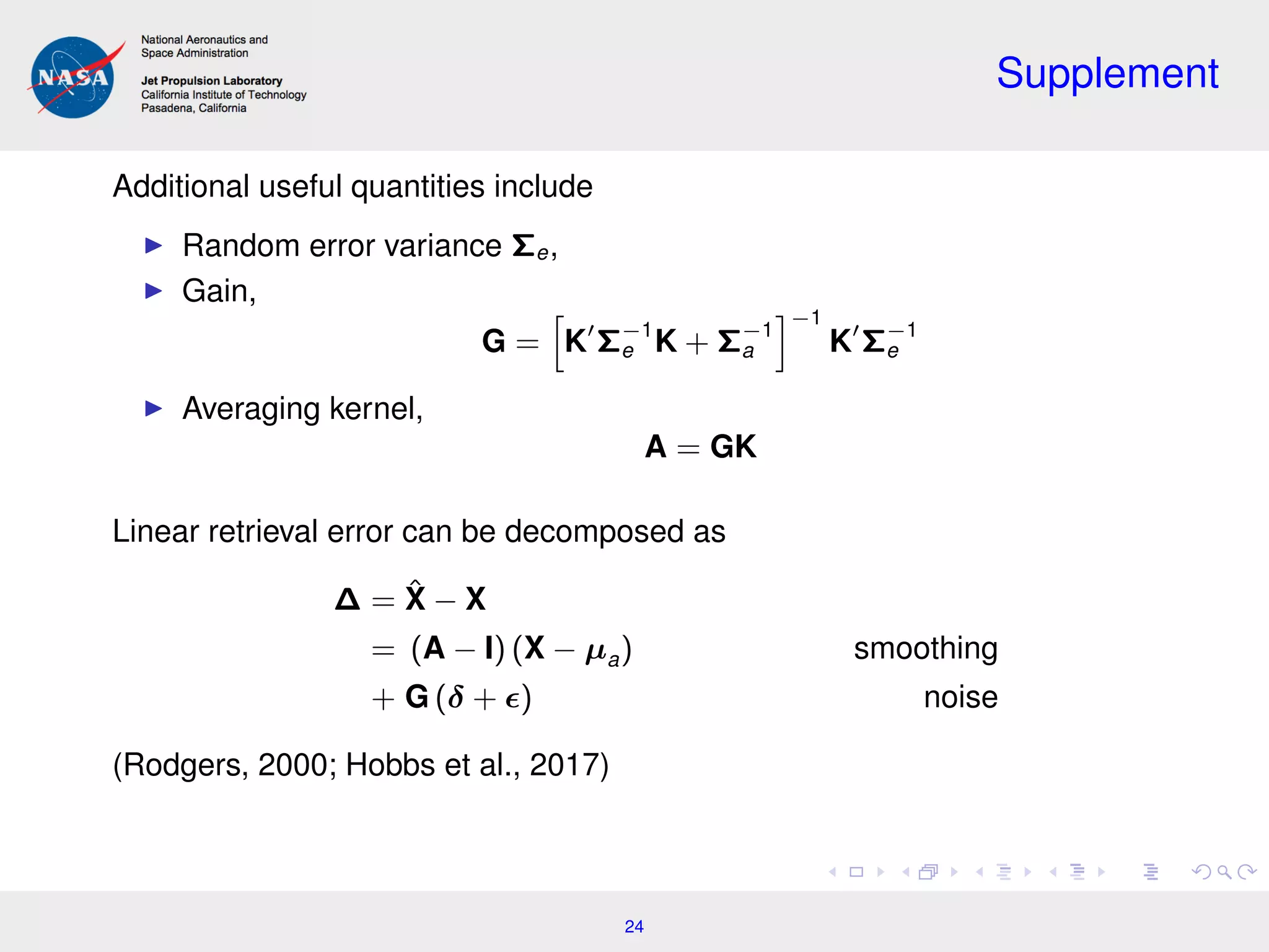
Consider a hierarchical model for a single pixel/footprint,
Xi ∼ MVN (µi , Σi )
Yi |Xi , B ∼ MVN (F(Xi , B), Σ )
Σ = Var ( i )
The conditional distribution can be used for inference on the state,
−2 ln[Xi |Yi , B] = (Yi − F(Xi , B))T
Σ−1
(Yi − F(Xi , B))
+ (Xi − µi )T
Σ−1
i (Xi − µi ) + constant.
6](https://image.slidesharecdn.com/hobbssamsitransition20180514-180515124846/75/CLIM-Transition-Workshop-Incorporating-Spatial-Dependence-in-Remote-Sensing-Inverse-Problems-Jon-Hobbs-May-14-2018-6-2048.jpg)
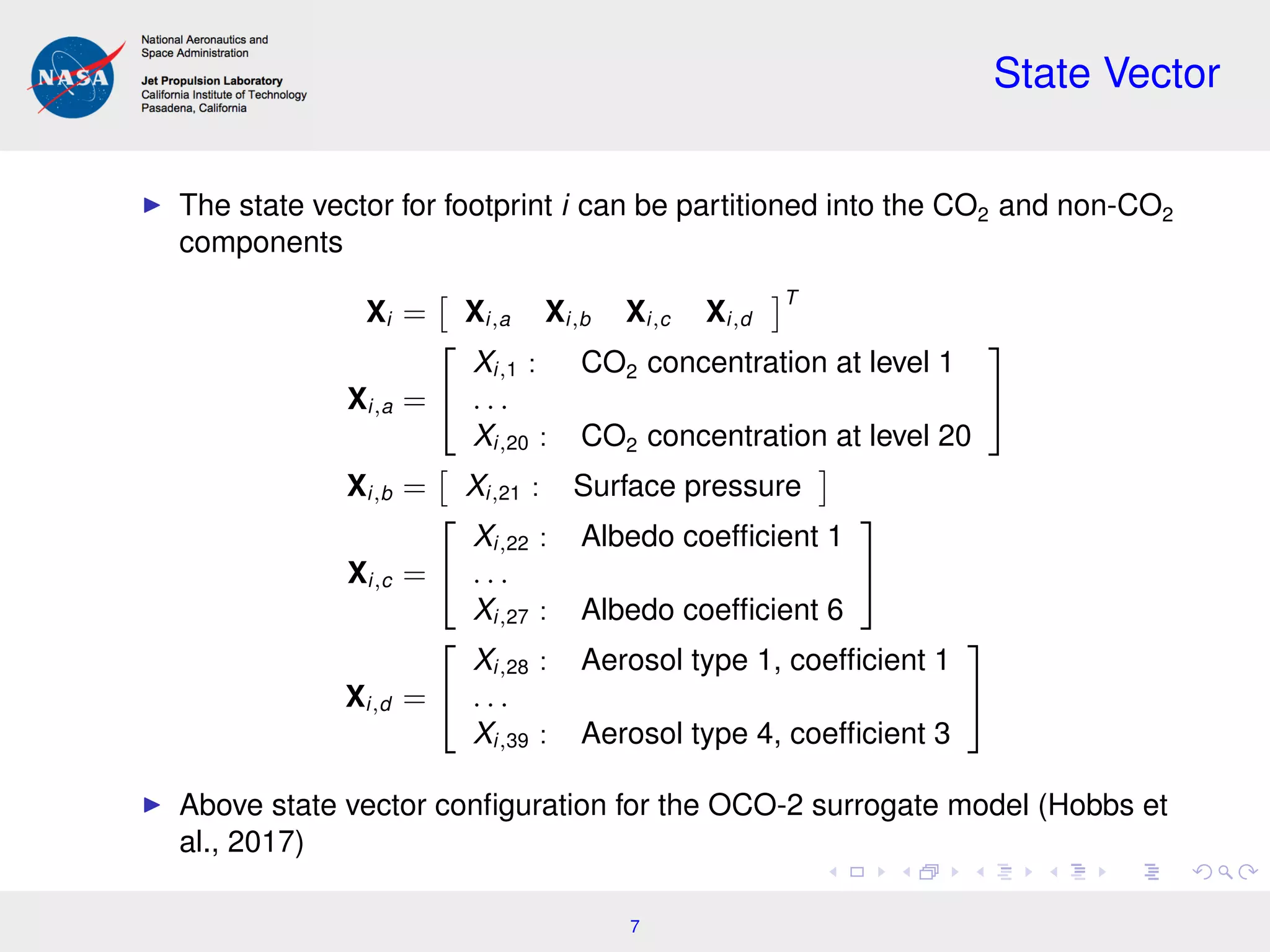
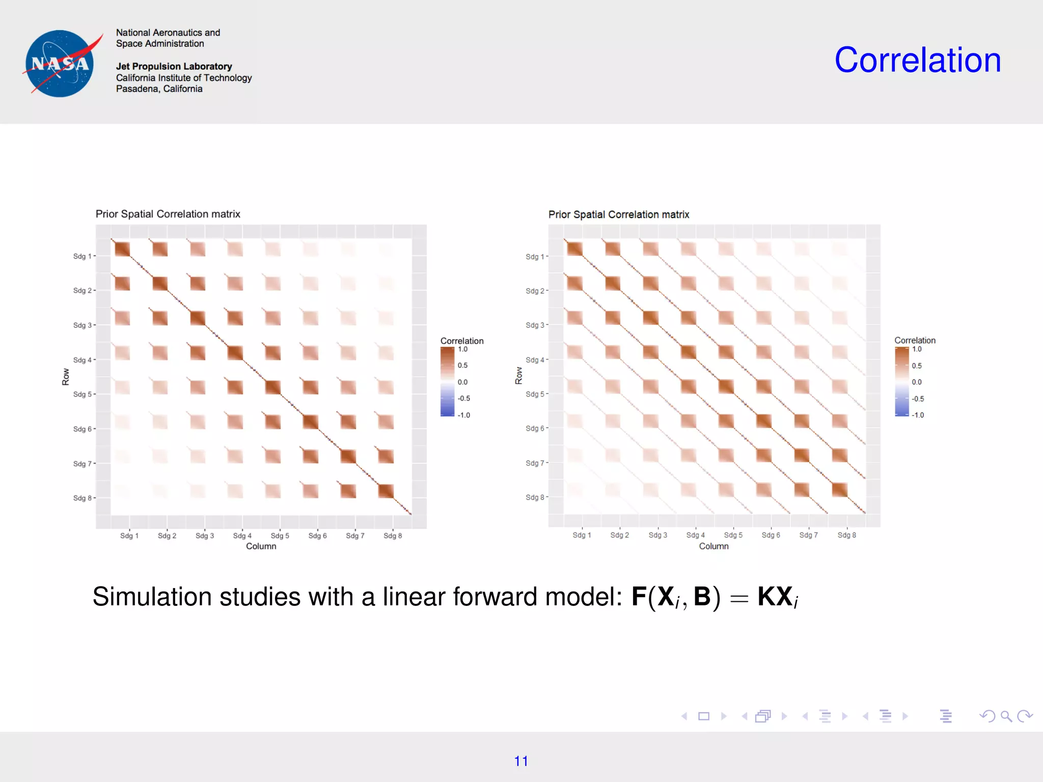
![Spatial Case
Consider, X = [X1 X2 . . . X8] , a collection of state vectors along an
eight-footprint transect:
X1 X2 X3 X4 X5 X6 X7 X8
Joint distribution
X ∼ MVN(µ, Σ)
Cost function
−2 ln[X|Y, B] =
8
i=1
(Yi − F(Xi , B))T
Σ−1
(Yi − F(Xi , B))
+ (X − µ)T
Σ−1
(X − µ) + constant.
Example of a multi-pixel retrieval (Dubovik et al., 2011)
9](https://image.slidesharecdn.com/hobbssamsitransition20180514-180515124846/75/CLIM-Transition-Workshop-Incorporating-Spatial-Dependence-in-Remote-Sensing-Inverse-Problems-Jon-Hobbs-May-14-2018-9-2048.jpg)
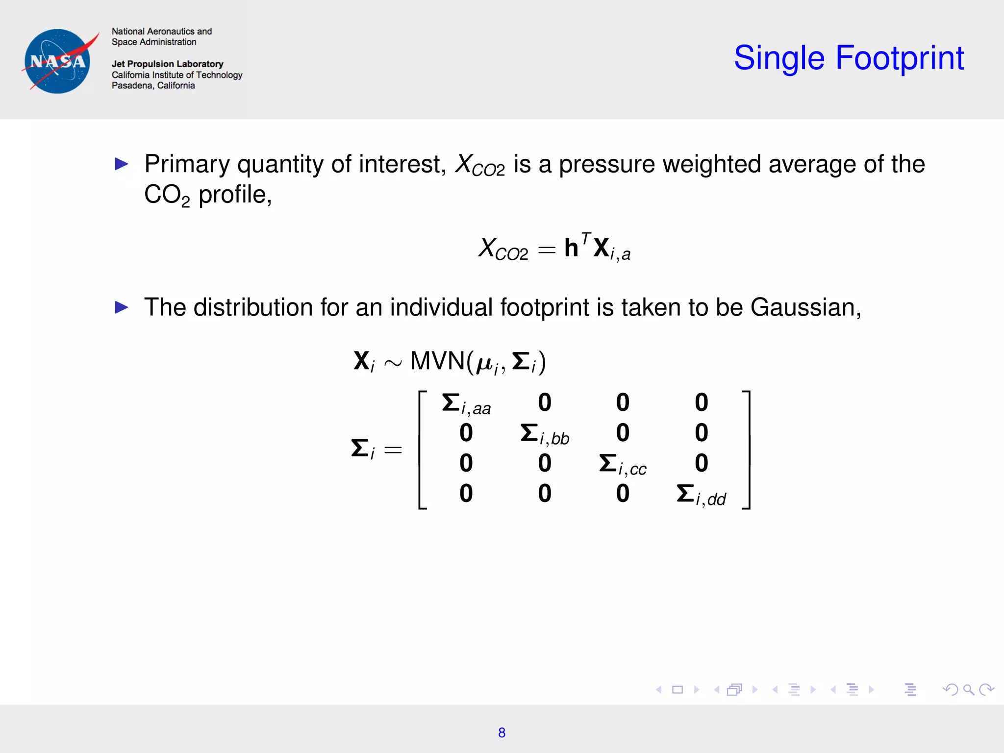
![Retrieval Error
q
q
q
q
q
q
q
q
q
q
q
q
q
q
q
q
q
q
q
q
q
q
q
q
q
q
q
q
q
q
q
q
0.5
0.6
0.7
0.8
FP1 FP2 FP3 FP4 FP5 FP6 FP7 FP8
Footprint
ErrorStdDev[ppm]
Model
q
q
q
q
NonSpat_Corr
NonSpat_Diag
Spatial_Corr
Spatial_Diag
Retrieval Error Variability
14](https://image.slidesharecdn.com/hobbssamsitransition20180514-180515124846/75/CLIM-Transition-Workshop-Incorporating-Spatial-Dependence-in-Remote-Sensing-Inverse-Problems-Jon-Hobbs-May-14-2018-14-2048.jpg)
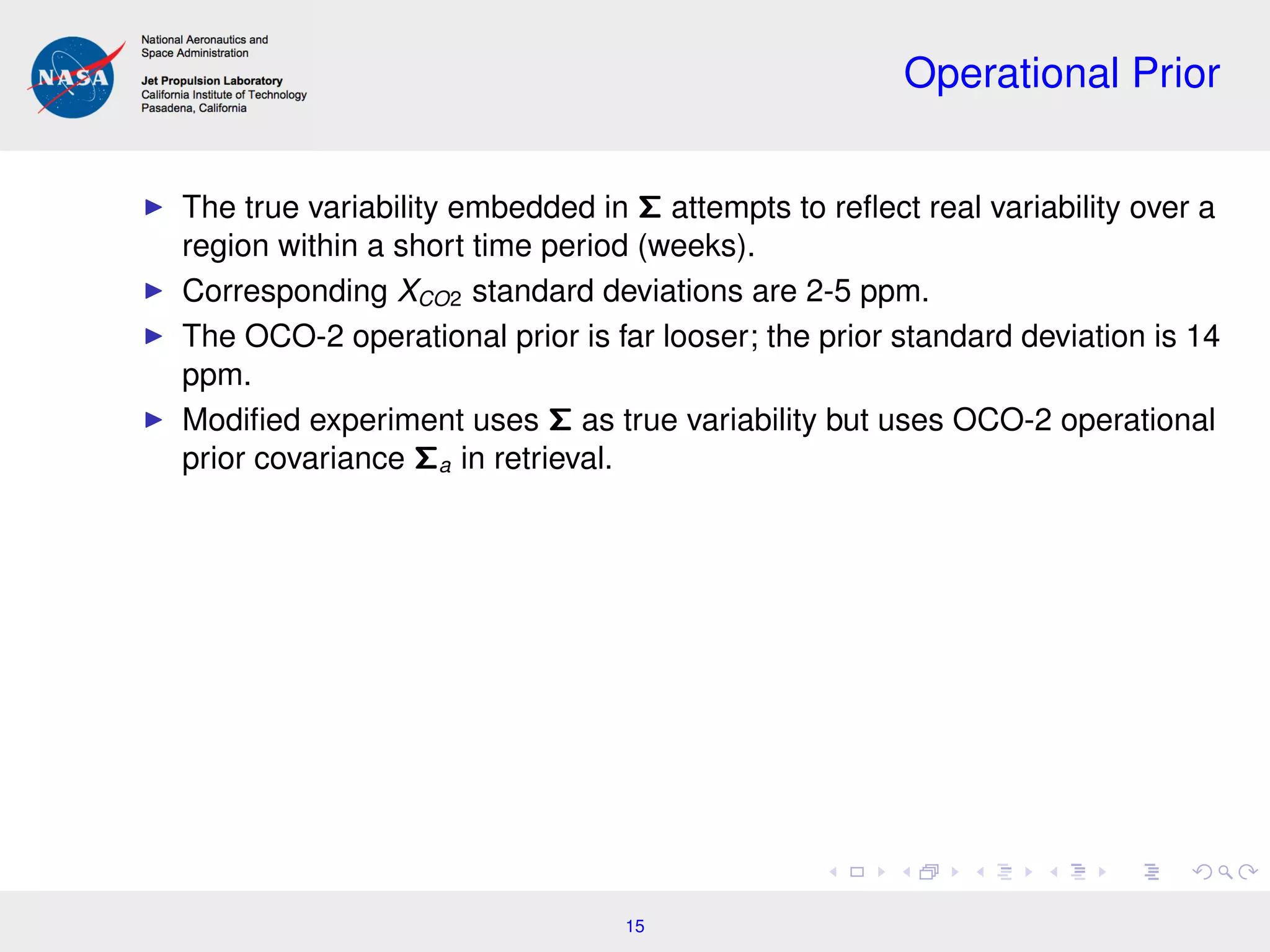
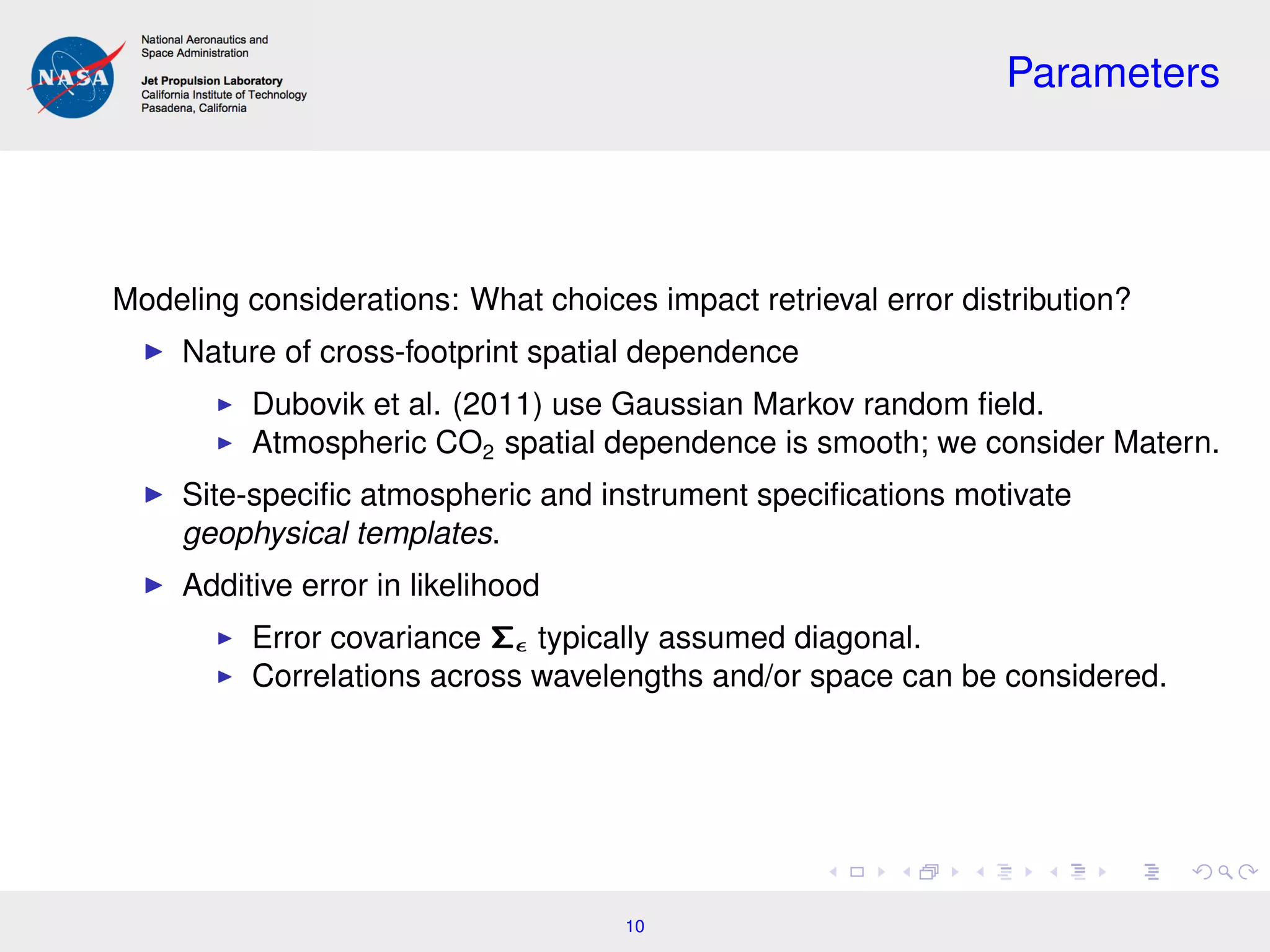
![Retrieval Error
q
q
q
q
q
q
q
q
q
q
q
q
q
q
q
q
q
q
q
q
q
q
q
q
q
q
q
q
q
q
q
q
0.8
1.0
1.2
1.4
FP1 FP2 FP3 FP4 FP5 FP6 FP7 FP8
Footprint
ErrorStdDev[ppm]
Model
q
q
q
q
NonSpat_Corr
NonSpat_Diag
Spatial_Corr
Spatial_Diag
Retrieval Error Variability
Operational Prior
16](https://image.slidesharecdn.com/hobbssamsitransition20180514-180515124846/75/CLIM-Transition-Workshop-Incorporating-Spatial-Dependence-in-Remote-Sensing-Inverse-Problems-Jon-Hobbs-May-14-2018-16-2048.jpg)
![Templates
q
q
q
q
q
q
q
q
q
q
q
q
q
q
q
q
q
q
q
q
q
q
q
q
0.0
0.5
1.0
02 04 05 06 08 09 10 11
Region
ErrorStdDev[ppm]
Model
q NonSpatial
Spatial
Region Errors
Retrieval error standard deviation for Footprint 4.
19](https://image.slidesharecdn.com/hobbssamsitransition20180514-180515124846/75/CLIM-Transition-Workshop-Incorporating-Spatial-Dependence-in-Remote-Sensing-Inverse-Problems-Jon-Hobbs-May-14-2018-19-2048.jpg)
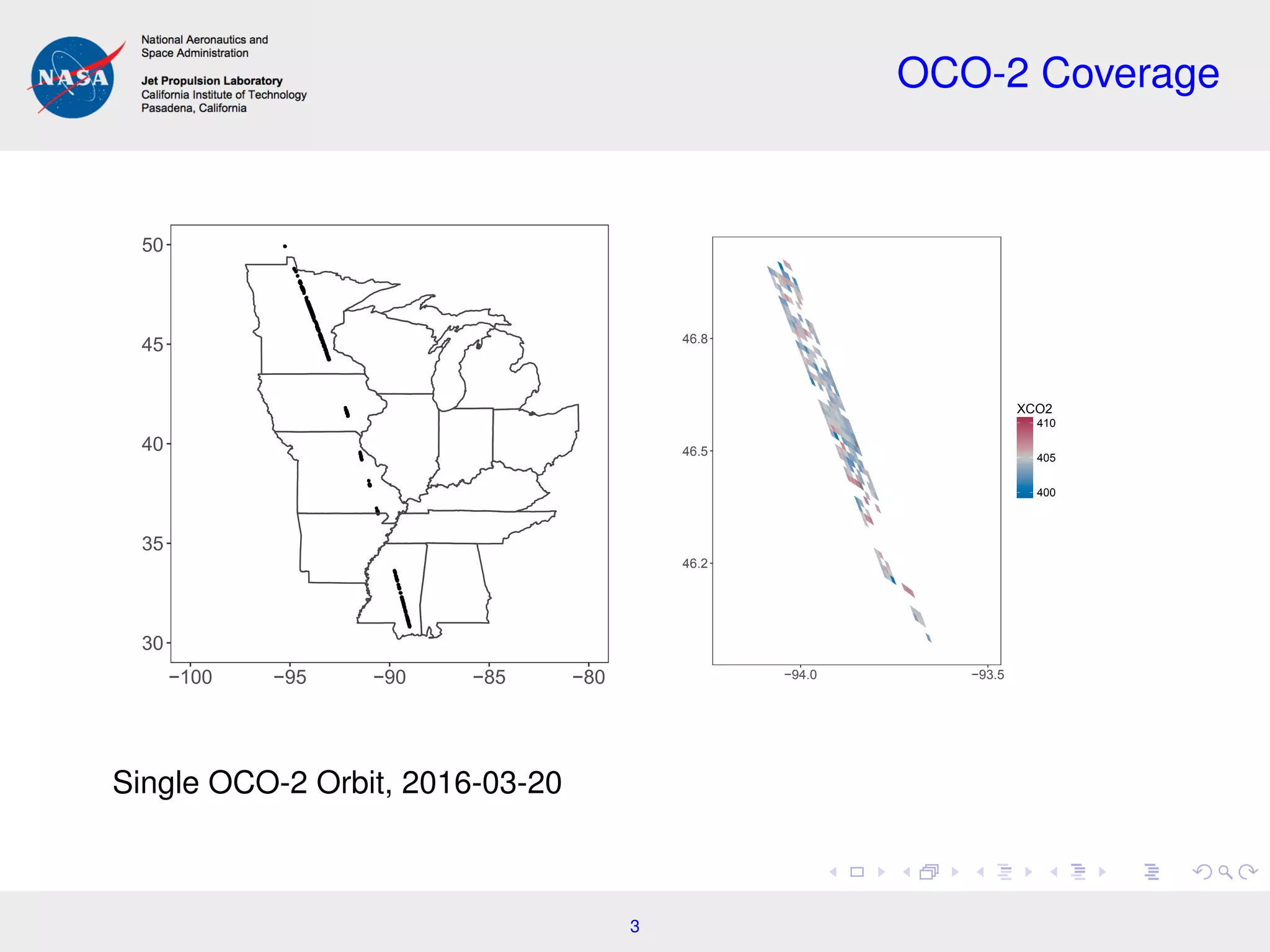
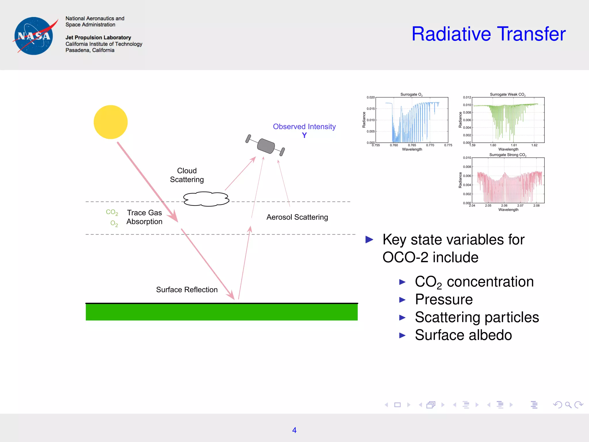
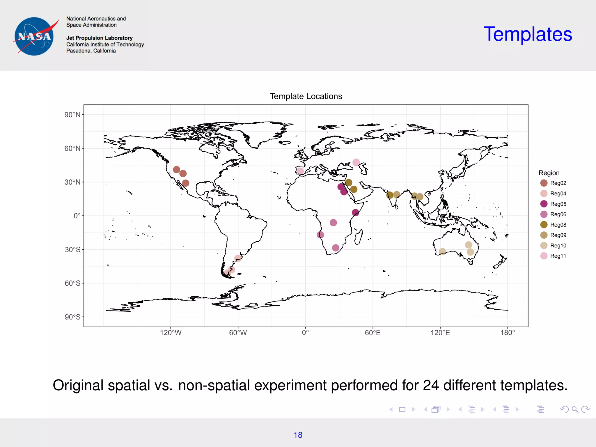
The document discusses incorporating spatial dependence into remote sensing inverse problems, particularly using data from NASA's OCO-2 satellite to improve estimates of atmospheric CO2. It outlines the statistical modeling and hierarchical approaches used to link measurement data to state vectors, highlighting the impact of spatial correlations on retrieval errors. Future work aims to refine these methods for larger spatial domains and enhance the realism of spatial process characterizations.


![Ica group 3[1]](https://cdn.slidesharecdn.com/ss_thumbnails/icagroup31-191026172214-thumbnail.jpg?width=640&height=640&fit=bounds)