Download to read offline
![Statistical Model
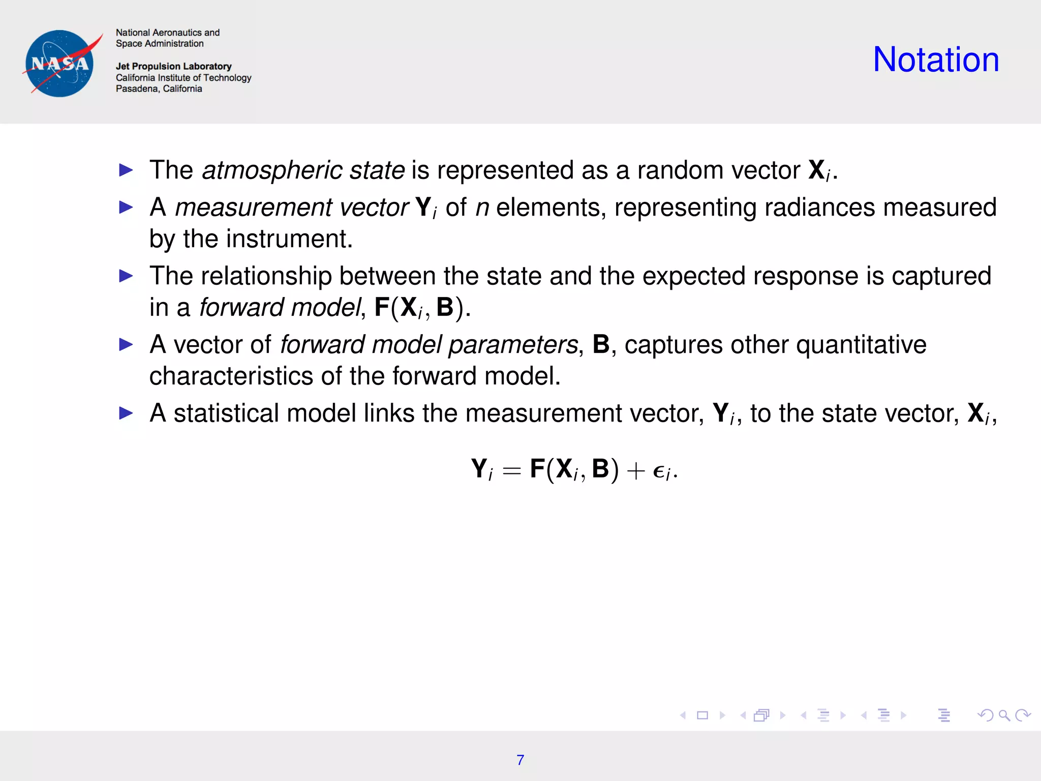
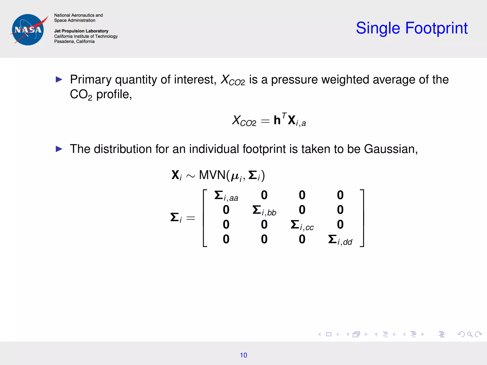
Consider a hierarchical model for a single pixel/footprint,
Xi ∼ MVN (µi , Σi )
Yi |Xi , B ∼ MVN (F(Xi , B), Σ )
Σ = Var ( i )
The conditional distribution can be used for inference on the state,
−2 ln[Xi |Yi , B] = (Yi − F(Xi , B))T
Σ−1
(Yi − F(Xi , B))
+ (Xi − µi )T
Σ−1
i (Xi − µi ) + constant.
8](https://image.slidesharecdn.com/hobbs-180228193818/75/CLIM-Program-Remote-Sensing-Workshop-Incorporating-Spatial-Dependence-in-Atmospheric-Carbon-Dioxide-Retrievals-from-HighResolution-Satellite-Data-Jonathan-Hobbs-Feb-12-2018-8-2048.jpg)
![Spatial Case
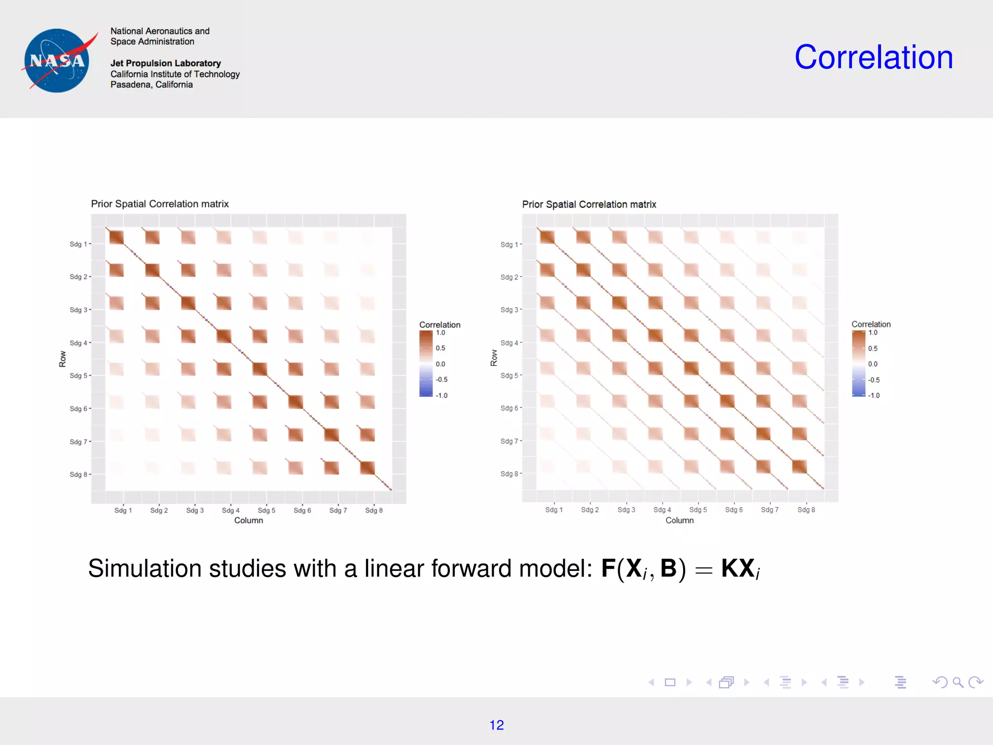
Consider, X = [X1 X2 . . . X8] , a collection of state vectors along an
eight-footprint transect:
X1 X2 X3 X4 X5 X6 X7 X8
Joint distribution
X ∼ MVN(µ, Σ)
Cost function
−2 ln[X|Y, B] =
8
i=1
(Yi − F(Xi , B))T
Σ−1
(Yi − F(Xi , B))
+ (X − µ)T
Σ−1
(X − µ) + constant.
11](https://image.slidesharecdn.com/hobbs-180228193818/75/CLIM-Program-Remote-Sensing-Workshop-Incorporating-Spatial-Dependence-in-Atmospheric-Carbon-Dioxide-Retrievals-from-HighResolution-Satellite-Data-Jonathan-Hobbs-Feb-12-2018-11-2048.jpg)
![Discussion
Future Work
Nonlinear case with iterative optimization
Joint inference for spatial dependence parameters in Σ, (Dubovik et al.,
2011; Wang et al., 2013)
Considerations for Data Systems
Initial results suggest the joint inference yields more precise (lower
standard error) estimates of XCO2.
Precision could improve with expanded spatial domain, but
computational cost also increases.
Can the trade-off be optimized?
Nonlinear optimization
Individual likelihood evaluations can be parallelized
Spatial prior density is relatively cheap to evaluate
−2 ln[X|Y, B] =
8
i=1
(Yi − F(Xi , B))T
Σ−1
(Yi − F(Xi , B))
+ (X − µ)T
Σ−1
(X − µ) + constant.
13](https://image.slidesharecdn.com/hobbs-180228193818/75/CLIM-Program-Remote-Sensing-Workshop-Incorporating-Spatial-Dependence-in-Atmospheric-Carbon-Dioxide-Retrievals-from-HighResolution-Satellite-Data-Jonathan-Hobbs-Feb-12-2018-13-2048.jpg)

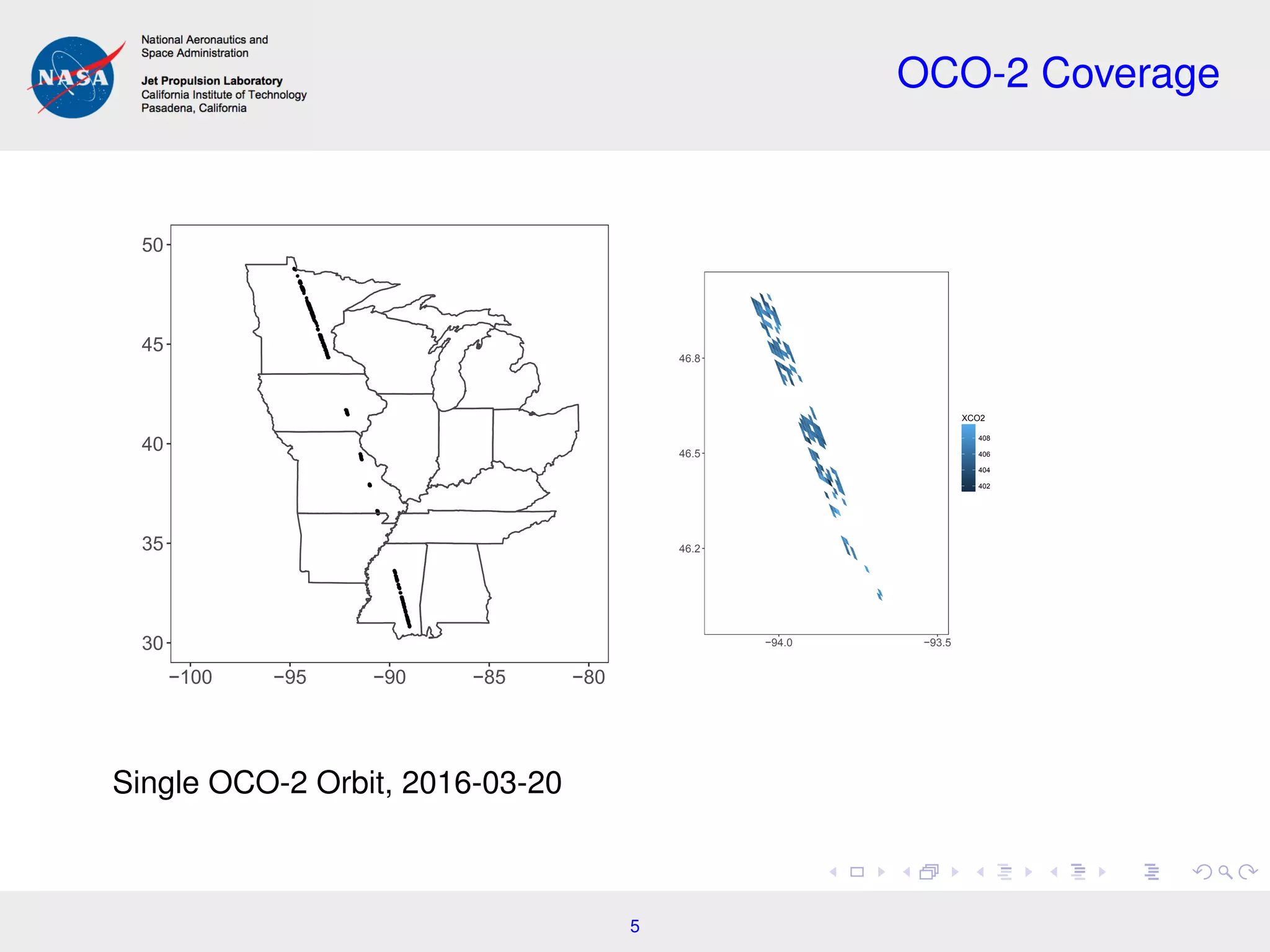
This document summarizes work on incorporating spatial dependence into atmospheric carbon dioxide retrievals from satellite data. It discusses using hierarchical Bayesian models to jointly analyze spatially correlated observations across multiple satellite footprints. This allows more precise carbon dioxide concentration estimates by borrowing strength between neighboring observations. Future work may optimize the tradeoff between precision and computational cost when analyzing larger spatial domains. The document also summarizes related work on using spatial unmixing models to estimate heterogeneous land properties like crop moisture levels from satellite imagery.