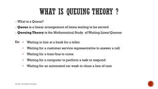
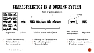
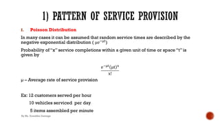
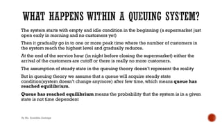
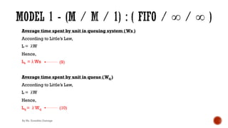
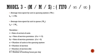
Queuing theory is the mathematical study of waiting lines in systems where demand for service exceeds the available resources. Key concepts include the patterns of arrivals and service, number of servers, queue discipline, size of the waiting area, and population size. Queuing models use notation like M/M/1 to describe characteristics like exponentially distributed inter-arrival and service times with a single server. Important metrics include the average number of customers in line and in the system, the average wait time, probability of idle servers, and server utilization. Little's law relates these metrics for systems in equilibrium.


![Ex: Answers
c) How long must a TV set be kept with the repairman relates to WS,
LS = λ WS
WS = LS /λ
But LS = θ / (1-θ) = (5/8) / [1- (5/8)] = 5 /3
WS = ( 5 /3 ) * ( 1 /10 ) = 1 /6 (eight hour day)
= 1/6 * 8 = 1 1/3 hrs
By Ms. Erandika Gamage](https://image.slidesharecdn.com/queuingtheory-final-230306131637-2ac7c2d6/85/Queuing-Theory-pdf-42-320.jpg)
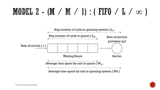
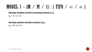
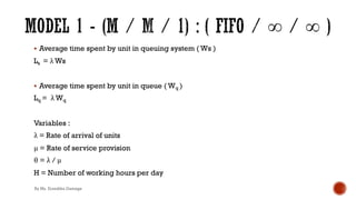
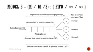
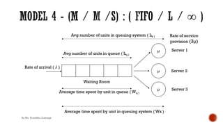
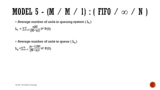
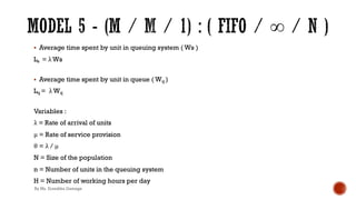
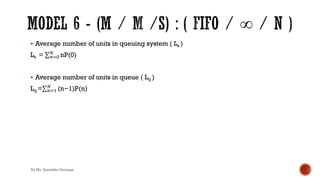
![Average number of units in queuing system ( Ls )
LS =
θ
(1− θL+1) {
'
'!(
- [LθL +
θL
'!(
] }
Average number of units in queue ( Lq )
Lq = LS - [1- P(0)]
By Ms. Erandika Gamage](https://image.slidesharecdn.com/queuingtheory-final-230306131637-2ac7c2d6/85/Queuing-Theory-pdf-46-320.jpg)
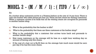
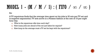
![Ex: Answers
Rate of arrival of customers (λ) = 14 per hour
Time taken for one hair cut = 4 mins
Number of haircuts completed in one hour = 60 / 4 = 15
Rate of service provision (μ) =15 per hour
Size of waiting room (L)= (5+1) = 6
θ = λ / μ =14 /15
(a) Probability that barber is idle = (1-θ) / (1- θL+1)
= (1-14/15) / [1- (14/15)7]
= (0.06669)/ (0.38304)
=0.174
By Ms. Erandika Gamage](https://image.slidesharecdn.com/queuingtheory-final-230306131637-2ac7c2d6/85/Queuing-Theory-pdf-49-320.jpg)
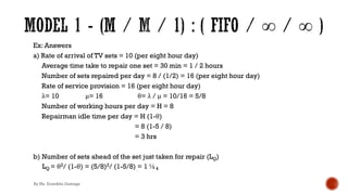
![Ex: Answers
(b) P (n) = θn (1-θ) / (1- θL+1)
If there are three customers then n=3
P (3) = θ3 (1-θ) / (1-θ7)
= (14/15)3 * (1-(14/15) / [1-(14/15)7]
= (14/15)3 * 0.174
=0.14146
By Ms. Erandika Gamage](https://image.slidesharecdn.com/queuingtheory-final-230306131637-2ac7c2d6/85/Queuing-Theory-pdf-50-320.jpg)
![Ex: Answers
(c) A customer arrive will leave and proceed to another barber shop only if the barber shop
is full.That is only if there are six customers in the shop.
So probability that a customer who arrives will leave for another barber shop is P (6)
P (6) = θ6 (1- θ) / (1- θL+1)
= (14/15)6 * [1-(14/15)] / [1-(14/15)7]
= (14/15)6 * 0.174
= 0.115
(d) Rate of arrival of customers = λ = 14 per hour
Number of customers that arrive on an 8 hour working day = 8*14 = 112
Probability of losing a customer = 0.115
Therefore number of customers lost per day = 112*0.115 = 12.88
By Ms. Erandika Gamage](https://image.slidesharecdn.com/queuingtheory-final-230306131637-2ac7c2d6/85/Queuing-Theory-pdf-51-320.jpg)
![Ex: Answers
(e) If there are five more chairs then all together there will be 10 waiting chairs and it will be a
limited waiting room size queue with size of waiting room as 11.
A customer will leave for another barber shop if the number of customers at the shop is 11.
Prob. that a customer arriving will leave for another shop = θ11 (1- θ) / (1- θL+1)
= θ11 (1- θ) / (1- θ12)
= (14/15)11 * [1-(14/15)] / [1-(14/15)12]
= 0.4681705 * (0.0666666) / (0.5630409)
= 0.0554334
Number of customers lost per day when (L =11) = 0.0554334 * 112
= 6.21
Number of customers lost per day when (L =6) = 112*0.115
= 12.88
Number of customers saved per day = 12.88 – 6.21 = 6.67
The increasing profit = Rs.6.67*50 = Rs. 333.00
By Ms. Erandika Gamage](https://image.slidesharecdn.com/queuingtheory-final-230306131637-2ac7c2d6/85/Queuing-Theory-pdf-52-320.jpg)
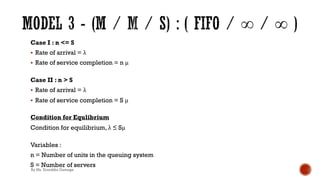
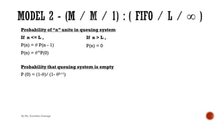
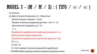
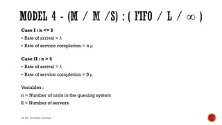
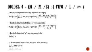
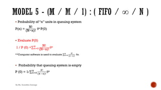
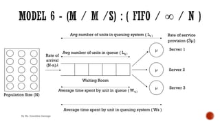
![§ Probability of “n” units in queuing system
Case I : n <= S
P (n) = (θn / n!) P (0)
P (S) = (θS / S!) P (0)
§ Evaluate P(0)
1 / P (0) = [ ∑&)*
+!'
(θn/n!) + (θS /S!) { 1 / (1-( θ /S)) } ]
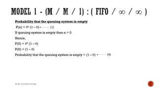
§ Probability that queuing system is empty
P (0) = 1/ [ ∑&)*
+!'
(θn /n!) + (θS /S!) { 1 / (1-( θ /S)) } ]
Case II : n > S
P (n) = (SS / S!) * (θ / S)n * P(0)
By Ms. Erandika Gamage](https://image.slidesharecdn.com/queuingtheory-final-230306131637-2ac7c2d6/85/Queuing-Theory-pdf-55-320.jpg)
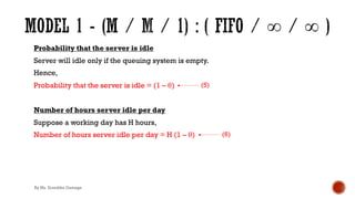
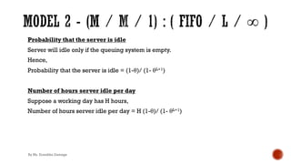
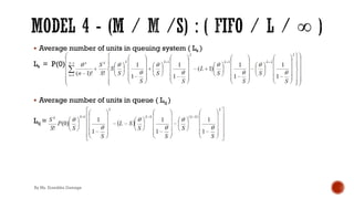
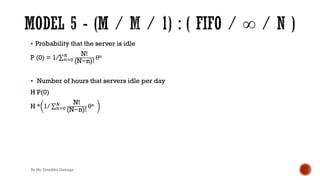
![§ Probability that all the servers are idle
P(0) = 1/ [ ∑&)*
+!'
(θn /n!) + (θS /S!) { 1 / (1-( θ /S)) } ]
§ Probability that “r” servers are idle
P (S-r)
§ Number of hours that servers idle per day
.∑,)*
+
Hr P (S−r)
By Ms. Erandika Gamage](https://image.slidesharecdn.com/queuingtheory-final-230306131637-2ac7c2d6/85/Queuing-Theory-pdf-56-320.jpg)
![Ex: Answers
(b) Number of servers (S)=2
Evaluate P (0)
1 / P (0) = [ ∑&)*
+!'
(θn/n!) + (θS /S!) { 1 / (1-( θ /S)) } ]
1 / P (0) = [∑&)*
&)'
(14 / 15) n /n!)+ (14 / 15)2 /2!) {1 / (1-(14 /30))}]
1 / P (0) = (14 / 15) 0 /0!) + (14 / 15) 1 /1!) + (14 / 15)2 / 2! * 30 / 16
1 / P (0) = 1 + (14 / 15) + (14 / 15)2 *(½) * (15 * 2) / 16
1 / P (0) = 1 + (14 / 15) + 142 / (15 * 16) = 2.75
1 / P (0) = 2.75
P (0) = 0.363636
Continued...
By Ms. Erandika Gamage](https://image.slidesharecdn.com/queuingtheory-final-230306131637-2ac7c2d6/85/Queuing-Theory-pdf-61-320.jpg)
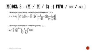
![Ex: Answers
(b) Ls = P(0) ∑&)'
+!' θn
&!' !
+
SS
S!
θ
S
.
S
' !
θ
S
+
θ
S
1
' !
θ
S
!
We have S = 2 , θ = 14 / 15 , (θ / S) = 14 / 30 , P (0) = 0.363636
Ls = 0.363636 ∑&)'
&)' (14 /15) n
&!' !
+
22
2!
14/15
2
1
2
' !
14/15
2
+
14/15
2
1
' !
14/15
2
!
LS = 0.363636 [(14 /15) 1 / 0! + 4 / 2 (14 / 30)2 {(60 / 16) + (14 / 30)(30 / 16)2}]
LS = = 1.1931805
Continued...
By Ms. Erandika Gamage](https://image.slidesharecdn.com/queuingtheory-final-230306131637-2ac7c2d6/85/Queuing-Theory-pdf-62-320.jpg)

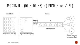
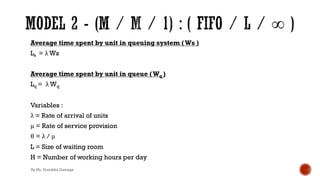
![§ Probability of “n” units in queuing system
Case I : n <= S
P (n) =
N!
(N−n)!n!
θn P(0)
P (S) =
N!
(N−S)!S!
θS P(0)
§ Evaluate P(0)
1 = ∑&)*
+!' N!
(N−n)!n!
θn P(0) + ∑&)+
3 N!
(N−n)!
(SS / S!) (θ / S)n P(0)
§ Probability that queuing system is empty
P (0) = 1/ [∑&)*
+!' N!
(N−n)!n!
θn P(0) + ∑&)+
3 N!
(N−n)!
(SS/ S!) (θ / S)n P(0) ]
Case II : n > S
P (n) =
N!
(N−n)!
(SS / S!)(θ / S)n P(0)
By Ms. Erandika Gamage](https://image.slidesharecdn.com/queuingtheory-final-230306131637-2ac7c2d6/85/Queuing-Theory-pdf-81-320.jpg)
![§ Probability that all the servers are idle
P (0) = 1/ [∑&)*
+!' N!
(N−n)!n!
θn P(0) + ∑&)+
3 N!
(N−n)!
(SS/ S!) (θ / S)n P(0) ]
§ Probability that “r” servers are idle
P (S-r) =
§ Number of hours that servers idle per day
.∑,)*
+
Hr P (S−r)
By Ms. Erandika Gamage](https://image.slidesharecdn.com/queuingtheory-final-230306131637-2ac7c2d6/85/Queuing-Theory-pdf-82-320.jpg)
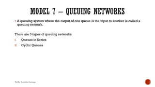
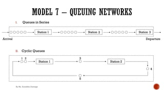
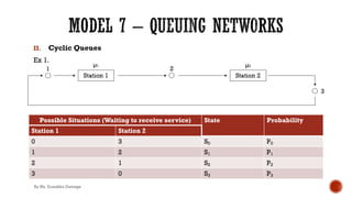
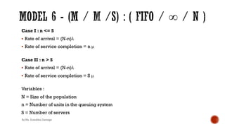
![II. Cyclic Queues
Ex 1.
State Balance Equation
S0 μ2P(0) = μ1P(1)
S1 (μ1+ μ2)P1 = μ2P0+ μ1P2
S2 (μ1+ μ2)P2 = μ1P3+ μ2P1
S3 μ1P3 = μ2P2
P0+ P1 + P2 + P3 = 1 [Sum of probabilities = 1]
We can solve the above equations and find P0,P1,P2 and P3 . once we find these measures
we can find expected number of units waiting to receive service from station 1 as,
(0 × P0+1× P1 +2 ×P2 +3× P3)
By Ms. Erandika Gamage](https://image.slidesharecdn.com/queuingtheory-final-230306131637-2ac7c2d6/85/Queuing-Theory-pdf-90-320.jpg)


![[DSC Europe 25] Ekaterina Bubenko - Behind the Curtain: How Data Roles Collab...](https://cdn.slidesharecdn.com/ss_thumbnails/anmv6x8dstqbbzchoklr-ekaterina-bubenko-behind-the-curtain-how-data-roles-collaborate-in-the-ai-era-a-260123083019-4b252ec7-thumbnail.jpg?width=640&height=640&fit=bounds)


![[DSC Europe 25] Predrag Maletic - Scaling AI in Banking – Our Strategic Journ...](https://cdn.slidesharecdn.com/ss_thumbnails/qu2onv0aruwlvqtygmxx-predrag-maletic-scaling-ai-in-banking-260123083019-6cf1da1d-thumbnail.jpg?width=640&height=640&fit=bounds)


![[DSC Europe 25] Josip Saban - Career building for data professionals.pptx](https://cdn.slidesharecdn.com/ss_thumbnails/zroflcttkm1vmli0txea-josip-saban-career-building-for-data-professionals-260123083019-587cdb8c-thumbnail.jpg?width=640&height=640&fit=bounds)


![[DSC Europe 25] Milos Belcevic - Product Professional's Journey to Full-Stack...](https://cdn.slidesharecdn.com/ss_thumbnails/1zovd6fgsycdg4wvgvls-milos-belcevic-product-professionals-journey-to-full-stack-product-developer-260123083019-d993120d-thumbnail.jpg?width=640&height=640&fit=bounds)


