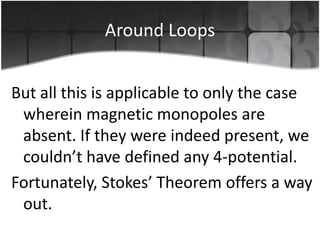
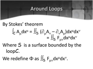
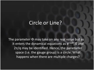
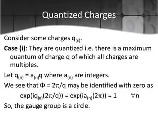
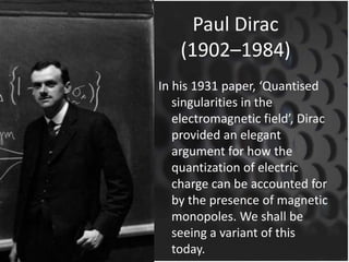
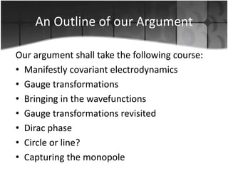
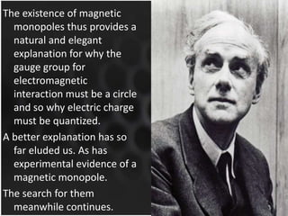
Student Technical Activities Body
The 2nd Annual Seminar Weekend
March 19, 2011

Charge Quantization
&
Magnetic Monopoles
Arpan Saha
Sophomore Undergraduate
Department of Physics
IIT Bombay
It seems that if one is working from
the point of view of getting beauty
in one's equations, and if one has
really a sound insight, one is on a
sure line of progress.
– Paul Adrien Maurice Dirac
Paul Dirac
(1902–1984)
In his 1931 paper, ‘Quantised
singularities in the
electromagnetic field’, Dirac
provided an elegant
argument for how the
quantization of electric
charge can be accounted for
by the presence of magnetic
monopoles. We shall be
seeing a variant of this
today.
An Outline of our Argument
Our argument shall take the following course:
• Manifestly covariant electrodynamics
• Gauge transformations
• Bringing in the wavefunctions
• Gauge transformations revisited
• Dirac phase
• Circle or line?
• Capturing the monopole
A List of Conventions
We adopt the following conventions:
• Units chosen so that c = ħ = 1
• Permittivity and permeability are subsumed into charge
density and current density.
• Vector and tensor components identified by putting an index
as superscript or subscript
• Latin indices run from 1 to 3 (three spatial dimensions).
• Greek indices run from 0 to 3 ( time + 3 spatial dimensions).
• Einstein Summation Convention: When an index occurs twice
(once as subscript and once as superscript) in a single term, it
is summed over.
• 0 := / x0 = / t, 1 := / x1, 2 := / x2 and 3 := / x3
Preliminaries
The permutation symbol or Levi-Civita
tensor
is defined by
0123 = 1
and that the tensor switches sign
whenever two indices are exchanged.
In particular, it is zero whenever an index is
repeated (no summation convention).
Preliminaries
The Minkowski metric
matrix
–1 0 0
0 1 0
0 0 1
0 0 0

is given by the
0
0
0
1
Manifestly Covariant
Electrodynamics
We are going to slightly rephrase Maxwell’s
Equations (in absence of any monopole) in terms
of the 4-potential and the field strength tensor.
The resulting equations are more elegant and
simpler to work with.
Maxwell’s Equations
E=
E = – B/ t
B=0
B = E/ t + j

(1)
(2)
(3)
(4)

E is the electric field, B is the magnetic field, is
the volume charge density and j is the surface
current density.
Magnetic Vector Potential
Since we have
B=0
We let
B=
A
(5)
where A is an ordinary 3-vector.
A is called the magnetic vector potential.
Scalar Potential
We substitute (5) into (2) to obtain
E=– (
A)/ t
i.e.
(E + A/ t) = 0
So we let
E + A/ t = –
(6)
is called the scalar potential.
4-Potential and 4-Current
The 3-vector A along with – as the zeroth (i.e.
time) component forms a 4-vector, whose
components we denote by A . This is called
the 4-potential.
The 3-vector j along with as the zeroth (i.e.
time) component forms a 4-vector, whose
components we denote by j . This is called the
4-current.
Field Strength Tensor
This is defined by
F = A – A
The full matrix is thus
0
E1
E2
E3

–E1
0
–B3
B2

–E2
B3
0
–B1

–E3
–B2
B1
0
Dual Field Strength Tensor
This is defined by
( F) = –(1/2)
F
where
is the permutation symbol and
is the Minkowski metric. The full matrix
is thus
0
B1
B2
B3

–B1
0
–E3
E2

–B2
E3
0
–E1

–B3
–E2
E1
0
Electrodynamics Rephrased
Maxwell’s Equations become
F = j
( F) = 0
Meanwhile, the Lorentz force is given by
dp /d = qF u
where p is the 4-momentum, is the proper
time, q is the charge of the particle and u is
the 4-velocity.
Gauge Transformations
Only the field strength tensor directly enters Maxwell’s
Equation. Hence, there is more than one possible
choice of the 4-potential that describes a given
physical situation. Transformations taking us from one
such 4-potential to another are called gauge
transformations.
Gauge Transformations
The transformed 4-potential must yield the
same field strength tensor as the original 4potential.
Consider a smooth scalar function of time and
space (x ).
Claim: The transformation A
A’ where
A’ = A +
is a gauge transformation.
Gauge Transformations
Proof: The transformed field strength tensor F’
is given by
F’ = A’ – A’
= (A +
) – (A +
)
= A – A
=F
The transformation A
A +
is, therefore,
a gauge transformation.
Bringing in the Wavefunctions
The 4-potential shall be incorporated into dynamical
equations describing the time-evolution of the
wavefunction of a particle. This shall then
describe the dynamics of the particle under
influence of an electromagnetic field.
Quantizing Electrodynamics
We start with the nonrelativistic Schrödinger
Equation for a particle of mass m in free
space.
(– 2/2m – i / t) = 0
The equation for a particle of spin zero and
charge q subjected to vector potential A and
scalar potential is
(–( – iqA)2/2m – i( / t + iq )) = 0
Quantizing Electrodynamics
When spin is nonzero (say ½), or the nonrelativistic
approximation breaks down, we have to turn to
more complicated equations such as the Pauli
Equation and the Dirac Equation.
But in all of them, space and time derivatives occur
in the combination ( – iqA) and ( / t + iq ).
That is, as per our convention, the derivatives occur
in the combination ( – iqA ).
Gauge Transformations Revisited
The fact that gauge transformations leave a physical
situation unchanged must carry over to quantum
mechanics. However, it turns out that the solution
to the dynamical equation in question changes
with a gauge transformation. But the change
constitutes only multiplication by a phase factor.
Transformation of Wavefunctions
The general dynamical equation may be stated as
f( – iqA ) = 0
For some function f. We make the following claim.
Claim: Given that under identical boundary conditions
f( – iqA ) = 0
f( – iqA’ ) ’ = 0
and that A’ = A +
then
’ = eiq
Transformation of Wavefunctions
Proof: To see this, all we need to consider is the
effect of the operator ( – iqA’ ) on eiq .
( – iqA’ )eiq = (eiq ) – iqA’ eiq
= iq( )eiq + eiq
– iq(A +
)eiq
= eiq ( – iqA )
Hence, f( – iqA’ )eiq = eiq f( – iqA )
=0
Transformation of Wavefunctions
This really shouldn’t be surprising, as it is
the modulus squared of the
wavefunction that has physical
significance.
Since | |2 =| ’|2, gauge transformations
do not change the physical state of a
given system.
Dirac Phase
How do we define the notion of phase parallelism of
two wavefunctions at a point in spacetime x ?
How do we define the same for two
wavefunctions at two different points in
spacetime x and x + dx so that it is invariant
over gauge transformations?
Wavefunctions at a Point
Two wavefunctions (1) and (2) are said to
be phase parallel (i.e. in phase) at x if
(1)(x ) = (2)(x )
Does the same idea work for wavefunctions
at two points?
No. Why?
Wavefunctions at Two Points
If

(1)(x

) = (2)(x + dx ), then after a gauge
transformation A
A +
, we have
exp(iq (x )) (1)(x )
exp(iq (x + dx )) (2)(x + dx )
The problem is easily rectified by stipulating that
at x and (2) at x + dx are phase parallel iff
exp(iqA dx ) (1)(x ) = (2)(x + dx )

(1)
Wavefunctions at Two Points
As a result, when a gauge transformation
A
A +
is performed,
exp(iq dx ) gets multiplied on both
sides.
This can be seen as a rule for parallel
transporting a wavefunction.
Around Loops
For finitely separated points P and Q joined by
a path in spacetime, we replace iqA dx by
an integral (iqA dx ).
This, in general, is path-dependent, so that
integrating around a loopC will give a
nonzero phase q where
= C A dx
The phase q is called the Dirac phase.
Around Loops
But all this is applicable to only the case
wherein magnetic monopoles are
absent. If they were indeed present, we
couldn’t have defined any 4-potential.
Fortunately, Stokes’ Theorem offers a way
out.
Around Loops
By Stokes’ theorem
A )dx dx
C A dx = S ( A –
= S F dx dx
Where S is a surface bounded by the
loopC.
We redefine as S F dx dx .
Circle or Line?
The parameter may take on any real value but as
it enters the dynamical equations as e–iq , 0 and
2 /q may be identified. Hence, the parameter
space (i.e. the gauge group) is a circle. What
happens when there are multiple charges?
Quantized Charges
Consider some charges q(n).
Case (i): They are quantized i.e. there is a maximum
quantum of charge q of which all charges are
multiples.
Let q(n) = a(n)q where a(n) are integers.
We see that = 2 /q may be identified with zero as
exp(iq(n)(2 /q)) = exp(ia(n)(2 )) = 1
n
So, the gauge group is a circle.
Non-quantized Charges
Case (ii): They are not quantized i.e. there is no
maximum quantum of charge q of which all
charges are multiples.
Hence there is no charge q such that
exp(iq(n)(2 /q)) = 1
n
So, gauge group is the real line.
We thus see that whether charges are quantized or
not is given by whether the gauge group is a circle
or a line.
Capturing the Monopole
Here we finally bring together all the strands and
establish a connection between charge
quantization and the existence of magnetic
monopoles.
Capturing the Monopole
Consider a closed surface S.
We can think of it as being
swept out by a family of
loopsCt passing through a
point P and parametrized
by a real number t.
The loops run from a point
loop at P to point loop at
P.

S

Ct

P
Capturing the Monopole
We compute for every loop.
It depends continuously on t, so it traces
a continuous curve in the gauge group
as t varies.
Since = 0 for a point loop, the curve
starts and ends at 0 i.e. it is closed.
Capturing the Monopole
What happens if you shrink the surface S to a
point? The closed curve in the gauge group
should collapse to a point as well.
Is this always possible?

Gauge group: Line

Gauge group: Circle
Capturing the Monopole
If the gauge group is a line, this is always
possible.
But, if the gauge group is a circle, this may
not be always possible.
In the latter case, something blocks us from
collapsing the surface S to a point.
That something is a magnetic monopole.
How do we see this?
Capturing the Monopole
For any loopCt, there is
some ambiguity in
choosing the surface
bounded by the loop.
In figure, for surfaces S (1)
and S (2), we have
(1) = S (1)F dx dx
(2) = S (2)F dx dx

S (1)

S (2)
The Monopole Captured
The net outward flux is given by (1) – (2).
If the closed curve in the gauge group can be
collapsed to a point, the above becomes zero.
If it makes a full circle around the circle gauge
group, because we identified 0 and 2 /q, we
have
(1) – (2) = (2 /q)N
Where N is an integer.
Dirac Quantization Condition
Hence, we conclude there is a magnetic
monopole inside whose magnetic
charge, being proportional to the
outward flux, is quantized in units
inversely proportional to q.
This is the celebrated Dirac quantization
condition.
The existence of magnetic
monopoles thus provides a
natural and elegant
explanation for why the
gauge group for
electromagnetic
interaction must be a circle
and so why electric charge
must be quantized.
A better explanation has so
far eluded us. As has
experimental evidence of a
magnetic monopole.
The search for them
meanwhile continues.
References
Aitchison, Hey, Gauge Theories in Particle Physics 3rd
Edn., Institute of Physics
Baiz, Muniain, Gauge Fields, Knots and Gravity,
World Scientific (1994)
Chan, Tsou, Some Elementary Gauge Theory
Concepts, World Scientific (1993)
Dirac, ‘Quantised Singularities in the Electromagnetic
Field’, Proceedings of the Royal Society of London:
Series A, Vol. 133, No. 821, Sept. 1, 1931
Kaku, Quantum Field Theory: A Modern Introduction,
Oxford University Press (1993)
Thank you!

Charge Quantization and Magnetic Monopoles

  • 1.
    Student Technical ActivitiesBody The 2nd Annual Seminar Weekend March 19, 2011 Charge Quantization & Magnetic Monopoles Arpan Saha Sophomore Undergraduate Department of Physics IIT Bombay
  • 2.
    It seems thatif one is working from the point of view of getting beauty in one's equations, and if one has really a sound insight, one is on a sure line of progress. – Paul Adrien Maurice Dirac
  • 3.
    Paul Dirac (1902–1984) In his1931 paper, ‘Quantised singularities in the electromagnetic field’, Dirac provided an elegant argument for how the quantization of electric charge can be accounted for by the presence of magnetic monopoles. We shall be seeing a variant of this today.
  • 4.
    An Outline ofour Argument Our argument shall take the following course: • Manifestly covariant electrodynamics • Gauge transformations • Bringing in the wavefunctions • Gauge transformations revisited • Dirac phase • Circle or line? • Capturing the monopole
  • 5.
    A List ofConventions We adopt the following conventions: • Units chosen so that c = ħ = 1 • Permittivity and permeability are subsumed into charge density and current density. • Vector and tensor components identified by putting an index as superscript or subscript • Latin indices run from 1 to 3 (three spatial dimensions). • Greek indices run from 0 to 3 ( time + 3 spatial dimensions). • Einstein Summation Convention: When an index occurs twice (once as subscript and once as superscript) in a single term, it is summed over. • 0 := / x0 = / t, 1 := / x1, 2 := / x2 and 3 := / x3
  • 6.
    Preliminaries The permutation symbolor Levi-Civita tensor is defined by 0123 = 1 and that the tensor switches sign whenever two indices are exchanged. In particular, it is zero whenever an index is repeated (no summation convention).
  • 7.
    Preliminaries The Minkowski metric matrix –10 0 0 1 0 0 0 1 0 0 0 is given by the 0 0 0 1
  • 8.
    Manifestly Covariant Electrodynamics We aregoing to slightly rephrase Maxwell’s Equations (in absence of any monopole) in terms of the 4-potential and the field strength tensor. The resulting equations are more elegant and simpler to work with.
  • 9.
    Maxwell’s Equations E= E =– B/ t B=0 B = E/ t + j (1) (2) (3) (4) E is the electric field, B is the magnetic field, is the volume charge density and j is the surface current density.
  • 10.
    Magnetic Vector Potential Sincewe have B=0 We let B= A (5) where A is an ordinary 3-vector. A is called the magnetic vector potential.
  • 11.
    Scalar Potential We substitute(5) into (2) to obtain E=– ( A)/ t i.e. (E + A/ t) = 0 So we let E + A/ t = – (6) is called the scalar potential.
  • 12.
    4-Potential and 4-Current The3-vector A along with – as the zeroth (i.e. time) component forms a 4-vector, whose components we denote by A . This is called the 4-potential. The 3-vector j along with as the zeroth (i.e. time) component forms a 4-vector, whose components we denote by j . This is called the 4-current.
  • 13.
    Field Strength Tensor Thisis defined by F = A – A The full matrix is thus 0 E1 E2 E3 –E1 0 –B3 B2 –E2 B3 0 –B1 –E3 –B2 B1 0
  • 14.
    Dual Field StrengthTensor This is defined by ( F) = –(1/2) F where is the permutation symbol and is the Minkowski metric. The full matrix is thus 0 B1 B2 B3 –B1 0 –E3 E2 –B2 E3 0 –E1 –B3 –E2 E1 0
  • 15.
    Electrodynamics Rephrased Maxwell’s Equationsbecome F = j ( F) = 0 Meanwhile, the Lorentz force is given by dp /d = qF u where p is the 4-momentum, is the proper time, q is the charge of the particle and u is the 4-velocity.
  • 16.
    Gauge Transformations Only thefield strength tensor directly enters Maxwell’s Equation. Hence, there is more than one possible choice of the 4-potential that describes a given physical situation. Transformations taking us from one such 4-potential to another are called gauge transformations.
  • 17.
    Gauge Transformations The transformed4-potential must yield the same field strength tensor as the original 4potential. Consider a smooth scalar function of time and space (x ). Claim: The transformation A A’ where A’ = A + is a gauge transformation.
  • 18.
    Gauge Transformations Proof: Thetransformed field strength tensor F’ is given by F’ = A’ – A’ = (A + ) – (A + ) = A – A =F The transformation A A + is, therefore, a gauge transformation.
  • 19.
    Bringing in theWavefunctions The 4-potential shall be incorporated into dynamical equations describing the time-evolution of the wavefunction of a particle. This shall then describe the dynamics of the particle under influence of an electromagnetic field.
  • 20.
    Quantizing Electrodynamics We startwith the nonrelativistic Schrödinger Equation for a particle of mass m in free space. (– 2/2m – i / t) = 0 The equation for a particle of spin zero and charge q subjected to vector potential A and scalar potential is (–( – iqA)2/2m – i( / t + iq )) = 0
  • 21.
    Quantizing Electrodynamics When spinis nonzero (say ½), or the nonrelativistic approximation breaks down, we have to turn to more complicated equations such as the Pauli Equation and the Dirac Equation. But in all of them, space and time derivatives occur in the combination ( – iqA) and ( / t + iq ). That is, as per our convention, the derivatives occur in the combination ( – iqA ).
  • 22.
    Gauge Transformations Revisited Thefact that gauge transformations leave a physical situation unchanged must carry over to quantum mechanics. However, it turns out that the solution to the dynamical equation in question changes with a gauge transformation. But the change constitutes only multiplication by a phase factor.
  • 23.
    Transformation of Wavefunctions Thegeneral dynamical equation may be stated as f( – iqA ) = 0 For some function f. We make the following claim. Claim: Given that under identical boundary conditions f( – iqA ) = 0 f( – iqA’ ) ’ = 0 and that A’ = A + then ’ = eiq
  • 24.
    Transformation of Wavefunctions Proof:To see this, all we need to consider is the effect of the operator ( – iqA’ ) on eiq . ( – iqA’ )eiq = (eiq ) – iqA’ eiq = iq( )eiq + eiq – iq(A + )eiq = eiq ( – iqA ) Hence, f( – iqA’ )eiq = eiq f( – iqA ) =0
  • 25.
    Transformation of Wavefunctions Thisreally shouldn’t be surprising, as it is the modulus squared of the wavefunction that has physical significance. Since | |2 =| ’|2, gauge transformations do not change the physical state of a given system.
  • 26.
    Dirac Phase How dowe define the notion of phase parallelism of two wavefunctions at a point in spacetime x ? How do we define the same for two wavefunctions at two different points in spacetime x and x + dx so that it is invariant over gauge transformations?
  • 27.
    Wavefunctions at aPoint Two wavefunctions (1) and (2) are said to be phase parallel (i.e. in phase) at x if (1)(x ) = (2)(x ) Does the same idea work for wavefunctions at two points? No. Why?
  • 28.
    Wavefunctions at TwoPoints If (1)(x ) = (2)(x + dx ), then after a gauge transformation A A + , we have exp(iq (x )) (1)(x ) exp(iq (x + dx )) (2)(x + dx ) The problem is easily rectified by stipulating that at x and (2) at x + dx are phase parallel iff exp(iqA dx ) (1)(x ) = (2)(x + dx ) (1)
  • 29.
    Wavefunctions at TwoPoints As a result, when a gauge transformation A A + is performed, exp(iq dx ) gets multiplied on both sides. This can be seen as a rule for parallel transporting a wavefunction.
  • 30.
    Around Loops For finitelyseparated points P and Q joined by a path in spacetime, we replace iqA dx by an integral (iqA dx ). This, in general, is path-dependent, so that integrating around a loopC will give a nonzero phase q where = C A dx The phase q is called the Dirac phase.
  • 31.
    Around Loops But allthis is applicable to only the case wherein magnetic monopoles are absent. If they were indeed present, we couldn’t have defined any 4-potential. Fortunately, Stokes’ Theorem offers a way out.
  • 32.
    Around Loops By Stokes’theorem A )dx dx C A dx = S ( A – = S F dx dx Where S is a surface bounded by the loopC. We redefine as S F dx dx .
  • 33.
    Circle or Line? Theparameter may take on any real value but as it enters the dynamical equations as e–iq , 0 and 2 /q may be identified. Hence, the parameter space (i.e. the gauge group) is a circle. What happens when there are multiple charges?
  • 34.
    Quantized Charges Consider somecharges q(n). Case (i): They are quantized i.e. there is a maximum quantum of charge q of which all charges are multiples. Let q(n) = a(n)q where a(n) are integers. We see that = 2 /q may be identified with zero as exp(iq(n)(2 /q)) = exp(ia(n)(2 )) = 1 n So, the gauge group is a circle.
  • 35.
    Non-quantized Charges Case (ii):They are not quantized i.e. there is no maximum quantum of charge q of which all charges are multiples. Hence there is no charge q such that exp(iq(n)(2 /q)) = 1 n So, gauge group is the real line. We thus see that whether charges are quantized or not is given by whether the gauge group is a circle or a line.
  • 36.
    Capturing the Monopole Herewe finally bring together all the strands and establish a connection between charge quantization and the existence of magnetic monopoles.
  • 37.
    Capturing the Monopole Considera closed surface S. We can think of it as being swept out by a family of loopsCt passing through a point P and parametrized by a real number t. The loops run from a point loop at P to point loop at P. S Ct P
  • 38.
    Capturing the Monopole Wecompute for every loop. It depends continuously on t, so it traces a continuous curve in the gauge group as t varies. Since = 0 for a point loop, the curve starts and ends at 0 i.e. it is closed.
  • 39.
    Capturing the Monopole Whathappens if you shrink the surface S to a point? The closed curve in the gauge group should collapse to a point as well. Is this always possible? Gauge group: Line Gauge group: Circle
  • 40.
    Capturing the Monopole Ifthe gauge group is a line, this is always possible. But, if the gauge group is a circle, this may not be always possible. In the latter case, something blocks us from collapsing the surface S to a point. That something is a magnetic monopole. How do we see this?
  • 41.
    Capturing the Monopole Forany loopCt, there is some ambiguity in choosing the surface bounded by the loop. In figure, for surfaces S (1) and S (2), we have (1) = S (1)F dx dx (2) = S (2)F dx dx S (1) S (2)
  • 42.
    The Monopole Captured Thenet outward flux is given by (1) – (2). If the closed curve in the gauge group can be collapsed to a point, the above becomes zero. If it makes a full circle around the circle gauge group, because we identified 0 and 2 /q, we have (1) – (2) = (2 /q)N Where N is an integer.
  • 43.
    Dirac Quantization Condition Hence,we conclude there is a magnetic monopole inside whose magnetic charge, being proportional to the outward flux, is quantized in units inversely proportional to q. This is the celebrated Dirac quantization condition.
  • 44.
    The existence ofmagnetic monopoles thus provides a natural and elegant explanation for why the gauge group for electromagnetic interaction must be a circle and so why electric charge must be quantized. A better explanation has so far eluded us. As has experimental evidence of a magnetic monopole. The search for them meanwhile continues.
  • 45.
    References Aitchison, Hey, GaugeTheories in Particle Physics 3rd Edn., Institute of Physics Baiz, Muniain, Gauge Fields, Knots and Gravity, World Scientific (1994) Chan, Tsou, Some Elementary Gauge Theory Concepts, World Scientific (1993) Dirac, ‘Quantised Singularities in the Electromagnetic Field’, Proceedings of the Royal Society of London: Series A, Vol. 133, No. 821, Sept. 1, 1931 Kaku, Quantum Field Theory: A Modern Introduction, Oxford University Press (1993)
  • 46.