1. The document discusses economic growth accounting and theories of economic growth. 2. Growth accounting explains that economic growth is due to increases in inputs like capital and labor as well as productivity increases from technological progress. The neoclassical growth model predicts economies will reach a steady state of constant per capita output and capital. 3. The document also examines factors that influence differences in economic growth rates between countries, such as capital accumulation, population growth, human capital development, and natural resources. It analyzes growth empirically and discusses implications of growth theory.

1. 1
GROWTH AND ACCUMULATION
MD Siyam HossainMD Siyam Hossain
Bangladesh Institute of Business & Technology.Bangladesh Institute of Business & Technology.
Narayangonj,DhakaNarayangonj,Dhaka
Dhaka,BangladeshDhaka,Bangladesh
www.facebook.com/mdsiyamhossain

2. 2
Economic Condition: Developed and less
developed countries
 Western has enormously higher incomes than
did their great grandparents
 People in industrialized nations are far
wealthier than people less developed countries
 Americans and Europeans had higher incomes
a century ago than people in poor countries
now
 Graph -1 shows GDP for four countries over
more than 150 years

3. 3
Graph has four striking characteristics:
a) It shows that in average in USA income increased
more than sixteen fold over this period
b) Japan was poor country before 2nd
World War.
Now it has a standard of living rough equal to
USA
c) Norwegian income has spurted in the last 25
years
d) Bangladesh was poor 150 years ago, grew very
slowly and remains that way today

4. 4
Figure 3-1: GDP Growth of USA, Japan, Norway and Bangladesh
GDP USA
Japan
Norway
Bangladesh

5. 5
Question is:
 What accounts for these differences? And
 What will determine our standard of living in future?
The answer of these questions are given by:
(i) Growth accounting and
(ii) Growth theory
Growth Accounting
 Growth accounting explains what part of growth in
total output is due to growth in different factors of
production (capital, labour, technology, etc.)
Growth Theory
 Growth theory explains how economic decisions
control the accumulation of factors of production
 Or, how rate of saving today affects stock of capital in
future

6. 6
1. GROWTH ACCOUNTING
General Explanation of Growth
Output grows through increases in:
(i) Inputs (K and N) and
(ii) Productivity due to (a) improved technology and
(b) a more able work force
Production Function
 Production function (I) provides a quantitative link
between inputs and outputs
 It relates level of output to level of inputs and level of
technology
Y = Aƒ(K, N) (1)
 Equation (1) is the functional equation of GDP
 Equation (1) is also called production function

7. 7
Where:
 N = Labour Force
 K = Capital (K) and
 A = Level of Technology
Equation (I) shows that output (Y) is a function of:
(i) Inputs (K and N) and
(ii) Level of technology (A)
Inputs
 More input means more output
 Increase in labour force (one input) increases output
(marginal product of labour/MPN)
 Increase in capital, the other input increases output
(marginal product of capital/MPK)

8. 8
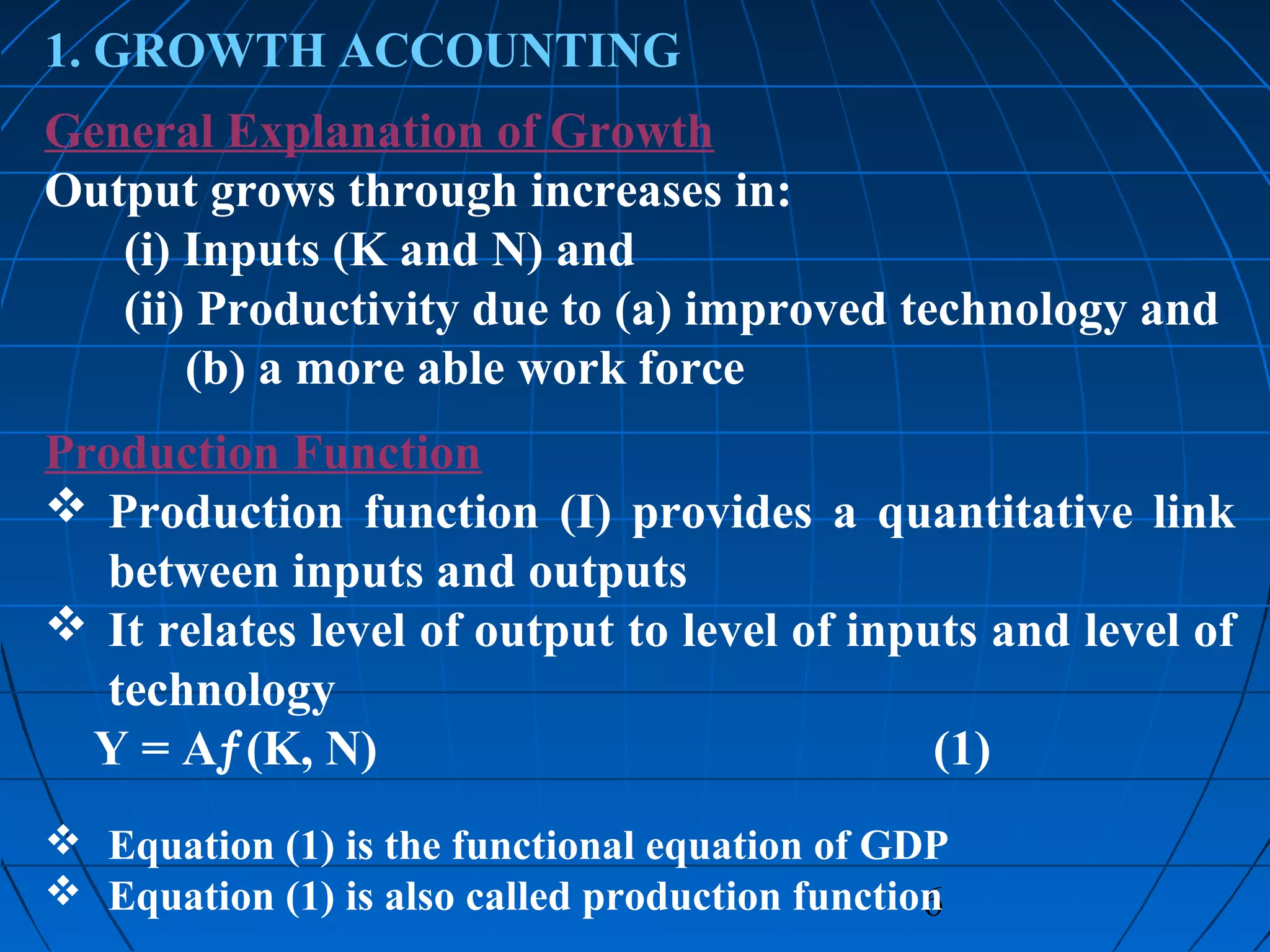
Level of technology
 A in production function is called
‘productivity’
 It is a more neutral term than ‘technology’
 Higher level of A means more output
 It means more output is produced for a given
level of inputs
 Production function (1) can be transformed
into a growth of output accounting equation
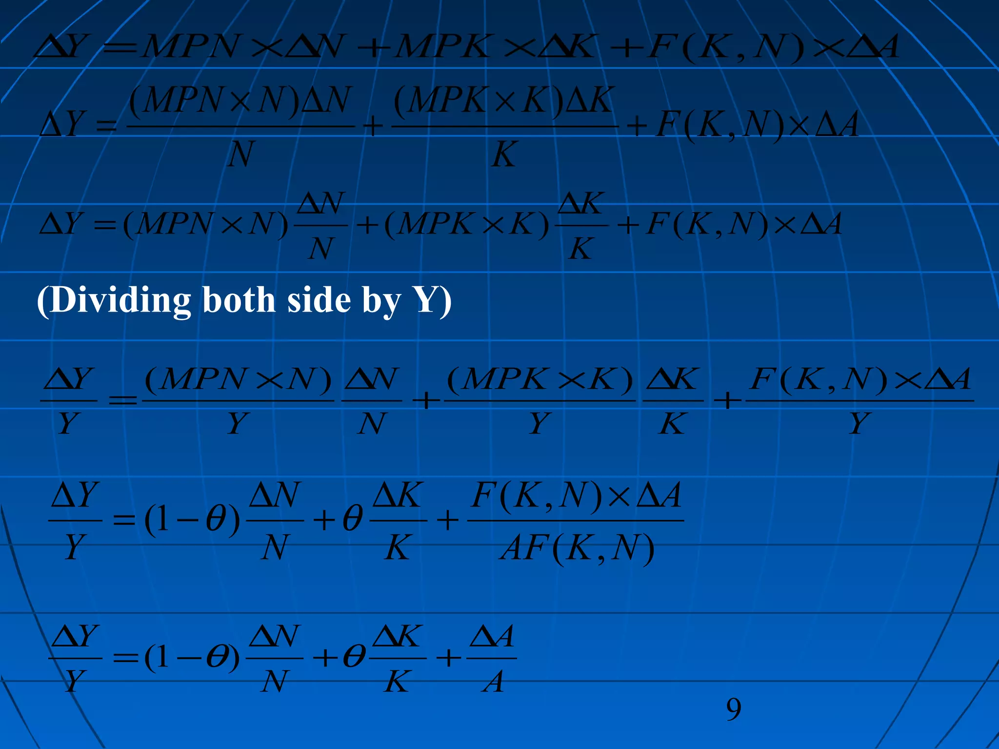
 ∆Y/Y = [(1 - θ) × ∆N/N] + (θ × ∆K/K) + ∆A/A (2)
It is called growth accounting equation

9. 9
(Dividing both side by Y)
ANKFKMPKNMPNY ∆×+∆×+∆×=∆ ),(
ANKF
K
K
KMPK
N
N
NMPNY ∆×+
∆
×+
∆
×=∆ ),()()(
Y
ANKF
K
K
Y
KMPK
N
N
Y
NMPN
Y
Y ∆×
+
∆×
+
∆×
=
∆ ),()()(
),(
),(
)1(
NKAF
ANKF
K
K
N
N
Y
Y ∆×
+
∆
+
∆
−=
∆
θθ
A
A
K
K
N
N
Y
Y ∆
+
∆
+
∆
−=
∆
θθ)1(
ANKF
K
KKMPK
N
NNMPN
Y ∆×+
∆×
+
∆×
=∆ ),(
)()(

10. 10
Where:
 (1 - θ) is the weight equal to labour’s share of income
 θ is weight equal to capital’s share of income
In words the equation can be written as
 Growth of Output=[(weight of labour share)×(labour
growth)]+[(weight of capital share)×(capital growth)] +
technical progress
 Equation 2 summarises the contribution of growth of
input and productivity to growth of output
It also says
 There is growth in total factor productivity, when we get
more output from same factors of production

11. 11
Example
 The capital share of income is 25% and that of labour
is 75%, which correspond to the value of US economy
Labour force growth is 1.2%, growth of the capital
stock is 3% and total factor productivity is 1.5%
annually What is the growth of the output?
Solution
Applying equation 2, we obtain a growth rate of:
 ∆Y/Y = (.75 × 1.2%) + (.25 × 3%) + 1.5% = 3.15%.
Conclusion
Growth of Output depends on:
(i) Kapital
(ii) Labour, and
(iii) Level of over all Technological Progress

12. 12
2. ACCOUNTING FOR GROWTH IN PER CAPITA OUTPUT
 Equation (2) helps calculating growth in total output
(absolute growth)
 But we are not really interested in total national output and
its growth
 Because it expresses little about development status and
living standard of a country
To know about real development level and compare it
with other countries:
 Per capita GDP is to be known
 As for instance, Norway is a rich country and India is a poor
country
 However, aggregate Indian GDP is higher than that of
Norway
 Standard of living refers to individual well-being
 Per capita GDP is the ratio of GDP to population

13. 13
Equation (2) helps deducing equation for accounting per
capita growth in output:
 ∆Y/Y = [(1 - θ) × ∆N/N] + (θ × ∆K/K) + ∆A/A
 ∆Y/Y = [∆N/N - θ×∆N/N] + (θ×∆K/K) + ∆A/A
 ∆Y/Y = ∆N/N - θ×∆N/N + (θ×∆K/K) + ∆A/A
 ∆Y/Y - ∆N/N= θ×∆K/K - θ×∆N/N + + ∆A/A
 ∆Y/Y- ∆N/N = θ×[∆K/K - ∆N/N] + ∆A/A
 ∆y/y = θ × ∆k/k + ∆A/A
 y = θ×∆k/k + ∆A/A
 y = θƒ(k) + ∆A/A (3)
Where:
 ∆Y/Y - ∆N/N = ∆y/y = per capita out put growth, and
 [Growth rate of per capita GDP equals the growth rate of
GDP minus growth rate of population]
 ∆K/K = ∆k/k + ∆N/N = ∆k/k = k = per capita capital growth
 [Growth rate of capital equals growth rate of per capita plus
growth rate of the population]

14. 14
Growth accounting equation (3) expresses that
per capita growth rate of GDP depends on:
 (i) Per capita capital growth (k) and
 (ii) Technological development (∆A/A)
 k is the number of machines per worker
 It is also called the capital-labour ratio
 It is a key determinant of the amount of output a
worker can produce
 Since θ is around .25, equation (3) suggests that:
 1% increase in amount of labour increases only
a quarter of 1% of per capita output
 In other word, to increase 1% of per capita
output (y), GDP, 4% capital has to be employed

15. 15
From growth accounting equations, technological change could
be calculated
If growth of GDP, Population (Labour) and Capital are known
We know that:
Hence:
Again we know that:
(3)
Hence:
(4)
A
A
K
K
N
N
Y
Y ∆
+
∆
+
∆
−=
∆
θθ)1(
K
K
N
N
Y
Y
A
A ∆
−
∆
−−
∆
=
∆
θθ )1(
A
A
k
k
y
y ∆
+
∆
×=
∆
θ
k
k
y
y
A
A ∆
×−
∆
=
∆
θ

16. 16
 Technological progress A is also called total
factor productivity
 Technological progress also cause increase of
labour productivity
 Such technological progress is called labour
augmenting technological progress
For labour augmenting technological progress
equation (3) is written as:
Hence:
(5)
A
A
k
k
y
y ∆
−+
∆
×=
∆
)1( θθ



 ∆
−
∆
−
=
∆
K
K
Y
Y
A
A
θ
θ1
1

17. 17
There is another production function of GDP
It is the Cobb-Douglas production function of GDP:
Here θ is the capital share to the GDP
[For USA θ = .20]
Here 1-θ is the labour share to the GDP
Cobb-Douglas production function is at same time GDP accounting
equation
If K and N are known the Y could be calculated
Cobb-Douglas production accounting equation could be
transferred into per capita form:
In functional form this equation could be written as:
y = ƒ(k)
θθ −
= 1
NAKY
θ
θ
θ
θ
θθ
θθ
Ak
N
K
A
N
K
ANAK
N
NAK
N
Y
y =





===== −
−1

18. 18
For labour augmenting technological
progress equation Cobb-Douglas
production accounting equation is written
as:
θθ −
= 1
)(ANKY
θθ −
= 1
NAKY
θθθ −−
= 11
NAKY
θθ
θ
−
−
= 1
1
NK
Y
A

19. 19
3. EMPIRICAL ESTIMATE OF GROWTH
 For growth capital accumulation is important, but technical
progress is more important
 In this regard Robert Solow studied period 1909-1949 in USA
 He concluded that over 80% of the growth was due to technical
progress
 Important determinants of per capita growth are technical
progress and capital accumulation
 Increased population means decrease GDP per capita even
though GDP increases
 More workers means more output, but output increases
proportionately slowly
 Each percentage growth of labour force leads to about .75-
percentage growth in output
 As output grows less quickly than numbers of workers, per
capita output falls

20. 20
4. FACTORS OTHER THAN CAPITAL AND LABOR
Besides capital and labour other important inputs for growth are:
(i) Natural resources and (ii) Human capital
Natural Resource
 Early prosperity of the US was due to abundant fertile
 From 1820 to 1870 arable land of USA grew at 1.41% annually
 Recent example of importance of natural resources is sharp
increase in Norwegian GDP
 From 1970-1990 Norway's per capita GDP rose from 61% to
77% of US per capita GDP
 This was due to the discovery and development of massive oil
reserves
 However, some empirical evidence suggests that:
 Countries with more natural resources generally do worse
 Explanation is: Some such countries squander their wealth

21. 21
Human Capital
 High investment leads to high income
 Question is, is there any relationship between human
capital and output
 In industrialized countries, qualified workers is more
important than unqualified labour
 Stock of unqualified workers could be increased by
investment in human capital
Adding human capital (H), production function could
be written as:
Y = AF(K,H,N) (4)
 Human capital is difficult to measure precisely
 However, length of schooling can serve as a proxy
for human capital

22. 22
Impact of Immigration
 Immigration boosts per capital output when skilled
workers enter the country
 From immigration USA has frequently benefited
 In USA qualified workers immigrated
Impact of Refugees
 Immigration consisting of refugees depresses per
capita output in the short run
 A factor of production adds to output growth only
when supply of this factor grows

23. 23
5. GROWTH THEORY - THE NEOCLASSICAL MODEL
There have been two periods of intense work on growth
theory:
(i) Late 1950s and 1960s and
(ii) Late 1980s and early 1990s
 Research in the first period produced
neoclassical growth theory
 This theory focuses on capital accumulation and
its link to savings
The other theory that focuses on the determinants of
technological progress is called:
Endogenous growth theory
This theory is studied in the next chapter

24. 24
Neo-classical growth theory
 Neo-classical growth theory begins with a
simplification of assumption
 It predicts that there is no technological progress in
the long run
 This implies that economy reaches a long-run level of
output and capital
 It is called the steady-state equilibrium

25. 25
Steady-state equilibrium
 Steady-state equilibrium is the combination of per
capita GDP and per capita capital where economy
remains at rest
It means in the steady state:
 Per capita economic variables are no longer changing
That is in steady state equilibrium:
 Per capita GDP does not grow [∆y = 0]
 Per capita capital does not grow [∆y = 0]

26. 26
Scope of Neo-classical growth theory
 Neo-classical growth theory studies transition
economy from its current position to steady state
It assumes that ultimately:
 There will no technological progress and
 Per capital GDP will remain unchanged
 Hence it develops first the growth model for steady
state and
 As a final step adds technological progress to the
model

27. 27
We know that
Production function in per capita terms for classical
model is written as:
 y = θƒ(k) + ∆A/A
If technological progress ∆A/A = 0 and θ = 0, then:
y = ƒ(k) (5)
 Here k is the capital-labour ratio
Considering technological progress; production function
can be expressed as:
y = ak or Y = aK

28. 28
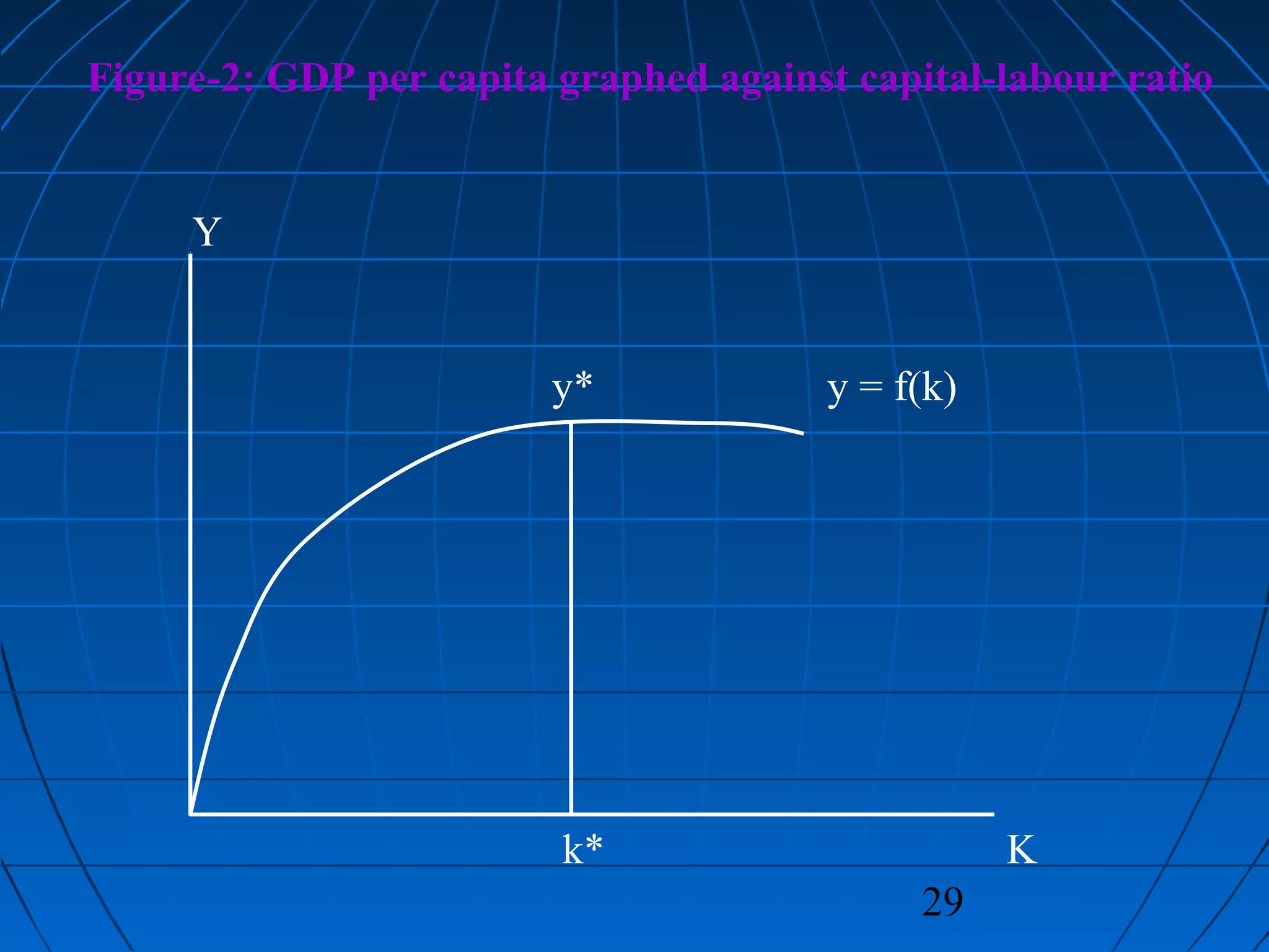
 Let us graph per capita GDP against capital-labour
ratio (Figure-2)
The graph shows that:
 As capital rises, output rises (marginal productivity of
capital is positive)
 However, output increases less at higher levels of
capital than at low levels
 [Following law of diminishing marginal productivity
of capital]
 Each additional machine adds to production, but adds
less than previous machine
 Law of diminishing marginal productivity is the key
explanation why the economy reaches a steady state
rather than growing endlessly

29. 29
Figure-2: GDP per capita graphed against capital-labour ratio
Y
y* y = f(k)
k* K

30. 30
5.1 Steady State
An economy is in a steady state:
 When per capita income and per capita capital are
constant (Figure-2)
 In steady state per capita income cannot be increased
more
 Steady-state value of per capita income = y*
 Steady-state value of per capita capital = k*
 At steady-state capital required for new workers and
machines worn out is just equal to saving generated
by economy
 At steady state levels of output saving and re-
investment balance

31. 31
Explaining the situation before steady state
Before steady state:
 Per capita output, y, could be increased
 Per capita capital, k, could be increased
 If saving is greater than investment requirement,
capital per worker and output rise
 If saving is less than investment requirement, capital
per worker and hence output fall
Conclusion
Have we:
 Steady-state value of per capita income, y*, and
 Steady-state value of per capita capital, k*
 We can examine transition path of economy from any
arbitrary point to steady state

32. 32
5.2 GROWTH IN NEOCLASSICAL MODEL
Investment required maintaining a certain level of
growth (capital per capita) depends on:
 (i) Population growth and (ii) Depreciation rate
 Let per capita capital required to maintain present
growth is k
 Let population grows at constant rate n (n = ∆N/N)
 Let the rate of depreciation is d
 Capital dk is required for new machinery to keep
present growth
 So, investment required to maintain level of growth
is (n + d) k

33. 33
 Let us now examine the link between saving and
growth in capital
 [Let there is no government sector and no foreign
trade or capital flows]
 Let the rate of saving is constant and s of income
 So, per capita saving is sy
 Since income equals production
 So, we can also write sy (and sy = sf (k)
Change in per capita capital (∆k) is excess of saving over
required investment:
 ∆k = sy - (n + d)k (6)

34. 34
We know that:
Steady state is defined by ∆k = O
So, steady state occurs at:
0 = sy - (n + d)k
sy = (n + d)k
At steady state the values of y and k are:
y* and k*
Hence
sy* = (n + d)×k* (7)
sy* = sf(k*) (8)

35. 35
Figure-3: Shows a graphical solution for the steady state
y
D y = f(k)
C (n+d)k
A sy
B
k0 k*
k

36. 36
Curve sy:
 Curve sy presents a constant proportion of output
 [Here s is the rate of saving of per capita capital and y is the
per capital output]
 Curve sy shows the level of saving at each capital-labour ratio
 Straight-line (n + d)×k
 Straight-line (n + d)×k shows amount of investment needed to
keep capital-labour ratio constant
 Intersection of the curve sy and the straight-line (n + d)×k at
point C means balance of saving and required investment at
steady state
 Here per capita capital is k*, that is steady-state per capita
capital (k*)
 Here per capita capital is k*, that is steady-state saving rate
(k*)
 Steady-state income (output) is read off the production
function at point D

37. 37
5.3 THE GROWTH PROCESS
Let us study the adjustment process that leads the
economy:
 From a initial capital-labour ratio to steady state
(Figure-3)
 Critical element in this transition process is:
 Rate of saving (s),
 Investment (k),
 Rate of depreciation (d), and
 Population growth (n)

38. 38
 Key to the neoclassical growth model is the saving, sy
 When sy exceeds the investment requirement (to
maintain running growth), k increases
 [When sy exceeds (n+d)×k, k increases]
 So, over time the economy grows (Figure-3)
 Let economy the starts at capital-output ratio ko
(Figure -3)
 At capital-output ratio ko-
investment at B is needed to
maintain current growth rate
 However, more is saved at point A,
 So, capital-output ratio increases and greater than ko-
 Hence, the economy growths and shifts left

39. 39
End of the Growth
 Adjustment process comes to a halt at point C
 Here the capital-labour ratio, k*, match the
investment requirement
 Beyond this point capital-labour ratio cannot be
more increased by saving
 And per capita output cannot also be increased more
 At this point so is saved as the growth rate demand
 If population increases, investment increases, but per
capita capital labour ratio remain constant
 At steady state, both k and y are constant
 At steady state growth rate is not affected by the
savings rate
 It is one of key results of neoclassical growth theory

40. 40
5.4 AN INCREASE IN THE SAVING RATE
 Let explain how increase in savings affects growth
 In short run, increase in savings rate raises growth
rate of output
 Let the economy is in equilibrium, at which saving
precisely matches investment requirement
 Let now people want to save a larger fraction of
income
 This causes an upward shift of savings schedule to
dashed schedule (Figure-4)
 Let at point C (Figure-4) we have initially
equilibrium
 Let now more is saved than is required to maintain
capital per head constant

41. 41
Figure-3: Shows a graphical solution for the steady state
y y1 = f(k1)
D y = f(k)
C1 (n+d)k
C sy
B
k0 k*
k

42. 42
 That means, enough is saved to allow capital stock per head to
increase
 Capital per head, k, rises until it reaches higher amount
 At point C1
(Figure-4) both capital per head and output per
head have risen
 However, economy has reached to its steady-state growth rate
 Now: Savings rate does not affect growth rate
 [Long run Neoclassical growth theory]
 In transition, higher savings rate increases growth rate of
output and per capita output
 It means, capital-labour ratio rises from k* to k**, steady state
 Only way to achieve an increase in capital-labour ratio is:
 Capital stock has to grow faster than the labour force
and depreciation