Downloaded 755 times
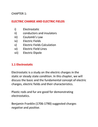
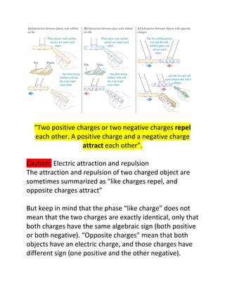


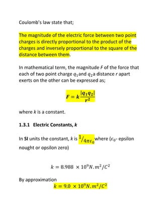

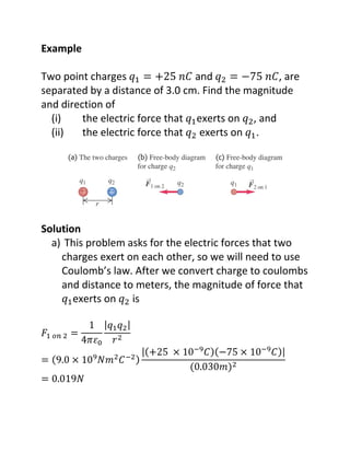


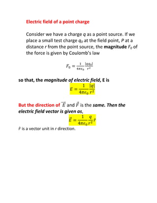
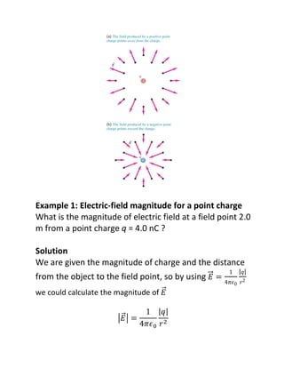


The document summarizes key concepts about electric charge and electric fields: 1) It defines electrostatics as the study of electric charges in a static or steady state condition. Some key topics covered include conductors and insulators, Coulomb's Law, electric fields, and electric field lines. 2) It explains Coulomb's Law which states that the magnitude of the electric force between two point charges is directly proportional to the product of the charges and inversely proportional to the square of the distance between them. 3) It defines the electric field as the electric force experienced by a test charge at a point in space, divided by the test charge. The direction of the electric field is the same as the