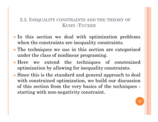
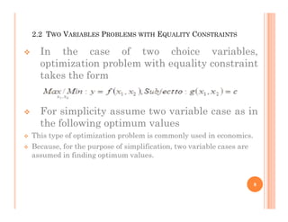
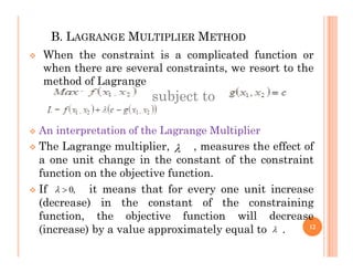
Chapter 2 discusses constrained optimization in economic contexts, where optimization must consider specific constraints such as resource availability. It explores one-variable and two-variable optimization problems with equality constraints using methods like elimination and Lagrange multipliers. The chapter emphasizes the importance of constraints on scope and method in maximizing or minimizing economic functions.

1. CHAPTER 2. CONSTRAINED
OPTIMIZATION
1

2. INTRODUCTION
 In economic optimisation problems, the
variables involved are often required to
satisfy certain constraints
 In case of unconstrained optimisation
problems, no restrictions have been made
regarding the value of the choice variables
regarding the value of the choice variables
 However, in reality optimisation of a certain
economic function should be in line with
certain resource requirement or availability
 This rises from the problem of scarcity
 For example:
 Maximisation of production should be subject to
the availability of inputs
2

3. CONT’D
 Minimisation of costs should also satisfy a certain
level of output
 The constraint in economics is the non-
negativity restrictions
 Although sometimes negative values may
be admissible, most functions in economics
be admissible, most functions in economics
are meaningful only in the first quadrant.
 Thus, this constraints should be
considered in the optimisation.
 The constraints in optimisation
 Constraints on the availability of the inputs
 None -ve solution
 Budget or money
3

4. CONT’D
 Constrained Optimization deals with optimization of
the objective function (the function to be optimized)
subject to constraints (restrictions).
 In case of a linear objective and constraint function, we
use the concept of linear programming model.
use the concept of linear programming model.
 However, when we face a non linear function, we use
the concept of derivatives for optimization. This
chapter focused on non linear constrained functions.
4

5. 2.1 ONE VARIABLE CONSTRAINED OPTIMIZATION
A. With Equality Constraint:
 Optimisation of one variable function subject to an
equality constraint takes the form,
Max(Min): y=f(x) subject to
The solution for this type of problem is
x
X 
)
(
* x
f
y 
B. Non-Negativity constraint
Max(Min):y=f(x) s.t x>0
 The optimum values of a function with non-
negativity constraint can be summarized as follows,
)
(
* x
f
y 

: '( ) 0 '( ) 0, 0
'( ) 0, 0
Max f x if f x x
if f x x
  
 
5

6. NONNEGATIVITY CONSTRAINT
 Graphically
 These three conditions can be consolidated in to:
f’(x1)  0 x1  0 and x1f’(x1) =0
 x1f’(x1)=0,  complementary slackness
 The three equations give us first order necessary
condition for extremum (local/global).
6

7. CONT’D
 Example:
2
3 7 2
. 0
Max y x x
st x
  


: '( ) 0 '( ) 0, 0
'( ) 0, 0
Min f x if f x x
if f x x
  
 
 In unconstrained optimization operation:
 F.O.C: f’(x)=-6x-7=0
 X=-7/6; However, imposing the non-negative constraint we
have:
 X*=0; and f(0)=-3(02)-7(0)+2=2
 f’(0)= -7<0
 It is maximized at this critical values
. 0
st x
7

8. 2.2 TWO VARIABLES PROBLEMS WITH EQUALITY CONSTRAINTS
 In the case of two choice variables,
optimization problem with equality constraint
takes the form
 For simplicity assume two variable case as in
 For simplicity assume two variable case as in
the following optimum values
 This type of optimization problem is commonly used in economics.
 Because, for the purpose of simplification, two variable cases are
assumed in finding optimum values.
8

9. CONT’D
 For example in maximization of utility using
indifference curve approach, the consumer is
assumed to consume two bundles of goods.
 Example:
Max utility, u(x1,x2),
Subject to budget constraint ,p1x1+ p2x2 =M
Subject to budget constraint ,p1x1+ p2x2 =M
 Two methods are commonly used for solving such
optimization problems with equality constraints.
A. Elimination and Direct Substitution Method
 This method is used for a two variables constrained
optimization problem with only one equality constraint.
 It is relatively simple method.
B. Lagrange Multiplier Method 9

10. A. ELIMINATION AND DIRECT SUBSTITUTION METHOD
 In this method, one variable is eliminated
using substitution before calculating the 1st
order condition.
 Consider the consumer problem in the above
example.
 Now x2 is expressed as a function of x1.
 Substituting this value, we can eliminate x2
from the equation. Using F.O.C
10

11. CONT’D
 Example: 1 2
max
x 4x 120
u x x
s.t

 
1 2
x 4x 120
s.t  
60
;
2
/
1
30
0
2
/
1
30
.
.
4
/
1
30
)
4
/
30
(
4
/
30
4
120
4
4
1
1
1
1
1
2
1
1
1
1
1
2
1
2
















x
x
x
MU
dx
du
C
C
F
x
x
x
x
u
x
x
x
x
15
4
/
60
30
2 


x
11

12. B. LAGRANGE MULTIPLIER METHOD
B. LAGRANGE MULTIPLIER METHOD
 When the constraint is a complicated function or
when there are several constraints, we resort to the
method of Lagrange
subject to
 An interpretation of the Lagrange Multiplier
 The Lagrange multiplier, , measures the effect of
a one unit change in the constant of the constraint
function on the objective function.
 If it means that for every one unit increase
(decrease) in the constant of the constraining
function, the objective function will decrease
(increase) by a value approximately equal to .

,
0


 12

13. EXAMPLE
 F.O.C
))
,
(
(
)
,
( 2
1
2
1 x
x
g
c
x
x
f
L 

 
0
)
,
(
)
,
( 2
1
1
2
1
1
1 

 x
x
g
x
x
f
L 
0
)
,
(
)
,
( 2
1
2
2
1
2
2 

 x
x
g
x
x
f
L 
0
)
,
( 2
1 

 x
x
g
c
L 
13

14. CONT’D
 We can express the optimal choices of variable as
implicit functions of the parameter c.
 Now, since the optimal value of L depends on we
may consider L to be a function of c.
,
, 2
1



x
and
x

)
(
*
)
(
)
(
*
*
2
2
1
c
c
x
x
c
x
x

 





,
, 2
1



x
and
x

may consider L to be a function of c.
 That is
1 2
( *, *, *)
L x x

14

15. CONT’D
 S.O.C. for a constrained optimization problem
 F.O.C. for
   
y
x
g
to
subject
y
x
f
Max ,
,
,
:
   
y
x
g
y
x
f
L ,
, 

    
y
x
g
y
x
f
L ,
, 


 
0
0
0
,
2
2








y
y
y
x
x
x
f
L
f
L
y
x
g
L




y
x
15

16. CONT’D
 To find the S.O.C find the second derivatives
Put these in matrix form to construct a Bordered
y
y
x
x g
L
g
L
L 

 

 ,
,
0
xy
xy
xy
xx
xx
xx g
f
L
g
f
L 
 


 ,
yy
yy
yy g
f
L 


 Put these in matrix form to construct a Bordered
Hessian and its determinant is denoted by .





















yy
yx
y
xy
xx
x
y
x
yy
yx
y
xy
xx
x
y
x
L
L
g
L
L
g
g
g
L
L
L
L
L
L
L
L
L 0





H
16

17. CONT’D
 The bordered Hessian is simply the plain Hessian
bordered by the first order derivatives of the constraint
with zero on the principal diagonal.
 Determinant Criterion for the sign definiteness of .
H
yy
yx
xy
xx
L
L
L
L


z
d 2
 Definiteness of the matrix is determined by looking at
the sign of principal minors, i.e.
 negative define alternating sign … for maximum
 same sign of positive definite …… for minimum 17
Max
L
L
g
L
L
g
g
g
iff
dg
to
subject
definite
Negative
definite
Positive
is
z
d
yy
yx
y
xy
xx
x
y
x











0
min
0
0
.
0
.
.
.
.
.
2

18. MORE THAN ONE EQUALITY CONSTRAINT
F.O.C.:
    and
c
x
x
x
g
to
subject
x
x
x
f
Min
Max 1
3
2
1
1
3
2
1 ,
,
,
,
,
,
,
:
/ 
  2
3
2
1
2
,
, c
x
x
x
g 
   
   
 
3
2
1
2
2
2
3
2
1
1
1
1
3
2
1 ,
,
,
, x
x
x
g
C
x
x
x
g
c
x
x
x
f
L 



 

 F.O.C.: 0
2
1
2
1
1
1
1
1 


 g
g
f
L 

0
2
2
2
1
2
1
2
2 


 g
g
f
L 

0
2
3
2
1
3
1
3
3 


 g
g
f
L 

  0
,
, 3
2
1
1
1
1


 x
x
x
g
C
L
  0
,
, 3
2
1
2
2
2


 x
x
x
g
C
L 18

19. MORE THAN ONE EQUALITY CONSTRAINT
 S.O.C
2
1
23
22
21
2
2
1
2
13
12
11
2
1
1
1
2
3
2
2
2
1
1
3
1
2
1
1
0
0
0
0
L
L
L
g
g
L
L
L
g
g
L
L
L
g
g
g
g
g
g
g
g
H 
 is one that contains L22 as the last element of its
principal diagonal
 is one that contains L33 as the last element of its
principal diagonal.
33
32
31
2
3
1
3 L
L
L
g
g

2
H

3
H
19

20. THE BORDERED HESSIAN
 Plain Hessian
xx xy
Z Z
Z Z 0 g g
 Bordered
Hessian: borders
will be ,
x y
g g
yx yy
Z Z 0 x y
x xx xy
y yx yy
g g
H g Z Z
g Z Z

20

21. SECOND ORDER CONDITION
Determinantal Criterion for sign definiteness:
2
2
>0
positive definite
is a subject to 0 iff
negative definite 0
or
0
positive definite 0
is a subject to 0 iff
negative definite 0
x y
x xx xy
y yx yy
H
d z dg
H
g g
d z dg g Z Z
g Z Z
 
   

   

   
 

  

  

  
y yx yy
g Z Z
21

22. EXAMPLE-1
 Find the extremum of
subject to 6
z xy x y
  
 First, form the Lagrangian function
(6 )
Z xy x y

   
(6 )
6 0 6
0 0
0
0
x
y
Z xy x y
Z x y x y
Z y or y
x
Z x


 


   

     

 
     
 
   
   

3 3 3 9
x y Z z
      
 By Cramer’s rule or some other method, we can find
22

23. CONT’D
Second order condition: first find the second order partial derivatives
0, 1, 0
and the border elements:
1, 1
Form the bordered Hessian Determinant:
0 1 1
xx xy yx yy
x y
Z Z Z Z
g g
   
 
0 1 1
1 0 1 2 0 9 is a maximum.
1 1 0
H z
    
23

24. EXAMPLE 2
 Find the extremum of
2 2
1 2 1 2
2 2
1 2 1 2
. . 4 2
The Lagrangian function is
(2 4 )
Necessary conditions:
z x x s t x x
Z x x x x

   
    
1 2 1 2
1 1 1
2 2 2
8
4 2 4
1 2
17 17 17 17
Necessary conditions:
2 4 0 4 2
2 0 2 0
2 4 0 4 2 0
Solution:
, , ,
Z x x x x
Z x or x
Z x x
x x Z z

 
 

     
 
 
     
 
 
     


     24

25. CONT’D
11 12 21 22
1 2
Second order condition: first find the second order partial derivatives
2, 0, 2
and the border elements:
1, 4
Form the bordered Hessian Determinant:
0 1 4
Z Z Z Z
g g
   
 
4
17
0 1 4
1 2 0 34 0
4 0 2
the value i
H
z
   
  s a minimum.
25

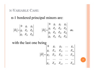
26. N-VARIABLE CASE:
1 2
( , , , )
n
z f x x x
 
1 2
( , , , )
n
g x x x c


1 2 1 2
( , , , ) [ ( , , , )]
n n
z f x x x c g x x x

  
 
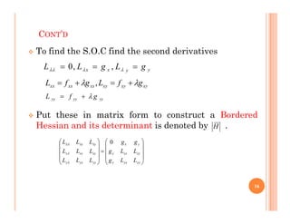
Objective function:
subject to
with
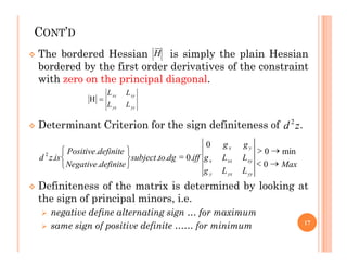
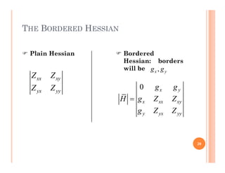
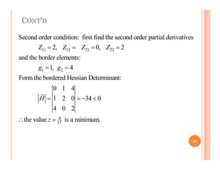
Given a bordered Hessian
Given a bordered Hessian
1 2
1 11 12 1
2 21 22 2
1 2
0 n
n
n
n n n nn
g g g
g Z Z Z
H g Z Z Z
g Z Z Z




    
 26

27. N-VARIABLE CASE:
n-1 bordered principal minors are:
1 2 3
1 2
1 11 12 13
2 1 11 12 3
2 21 22 23
2 21 22
0
0
etc.
g g g
g g
g Z Z Z
H g Z Z H
g Z Z Z
g Z Z
g Z Z Z
 
2 21 22
3 31 32 33
g Z Z Z
with the last one being
.
1 2
1 11 12 1
2 21 22 2
1 2
0 n
n
n
n n n nn
g g g
g Z Z Z
H g Z Z Z
g Z Z Z




    

27

28. N-VARIABLE CASE:
1 2 0
n
Z Z Z Z
     

1 2 0
n
Z Z Z Z
     

Condition Maximum Minimum
First order
necessary condition 1 2 3 ... 0
n
L L L L L
      1 2 3 ... 0
n
L L L L L
     
.
Second order
sufficient condition 2 3 4 5
0, 0, 0, 0,
...,( 1) 0
n
n
H H H H
H
   
 
2 3
0, 0,... 0
n
H H H
  
28

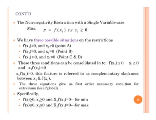
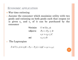
29. EXAMPLE: LEAST COST COMBINATION OF INPUTS
K L
C P K P L
 
0
( , )
Q K L Q

Minimize :
subject to:
First Order Condition:
0
0
[ ( , )]
( , ) 0
0
0
K L
K K K
L L L
K K
L L
Z P K P L Q Q K L
Z Q Q K L
Z P Q
Z P Q
P Q
P Q




   
  
  
  

First Order Condition:
29

30. CONT…..
2 2
0
( 2 ) 0
K L
KK KL KK L KL K L LL K
LK LL
Q Q
H QK Q Q Q Q Q Q Q Q Q
QL Q Q
  
 
      
 
Second order condition:
Therefore, since |H|<0, we have a minimum.
30

31. SELF ACTIVITY
1. The production function of the firm is given as: .
Labor costs 96 dollar per unit and capital costs 162 dollar
per unit so that the firm decides to produce 3456 units of
output (Q).
a. Determine the amount of labor and capital that should be
utilized so as to minimize costs.
b. Calculate the minimum cost and economically interpret
lambda.
2. Given the objective function as f(x,y,z)=4xyz2
Subject to x+y+z=56
3 1
4 4
64
Q L K

Subject to x+y+z=56
a. Use lagrange multiplier to calculate the critical values
of the choice variables.
b. Check whether the objective function has maximum or
minimum value at the obtained critical values using
bordered hessian test.
c. Estimate the effect on the value of objective function
for one unit change in the constraint function.
31

32. 2.3. INEQUALITY CONSTRAINTS AND THE THEORY OF
KUHN -TUCKER
2.3. INEQUALITY CONSTRAINTS AND THE THEORY OF
KUHN -TUCKER
 In this section we deal with optimization problems
when the constraints are inequality constraints.
 The techniques we use in this section are categorized
under the class of nonlinear programing.
 Here we extend the techniques of constrained
 Here we extend the techniques of constrained
optimization by allowing for inequality constraints.
 Since this is the standard and general approach to deal
with constrained optimization, we build our discussion
of this section from the very basics of the techniques -
starting with non-negativity constraint.
32

33. CONT’D
 Nonnegativity Restrictions: Consider a problem with
nonnegativity restrictions on the choice variables, but with no
other constraints.
 where the function f is assumed to be differentiable.
 Three possible situations may arise: interior solution, boundary
 Three possible situations may arise: interior solution, boundary
solution, and corner solution with negative FOC.
 These scenarios are shown in the figure below.
33

34. CONT’D
 The Non-negativity Restriction with a Single Variable case
Max:
 We have three possible situations on the restrictions
 f’(x1)=0, and x1>0 (point A)
 f’(x1)=0, and x1=0 (Point B)
 f’(x1)< 0, and x1=0 (Point C & D)
1 1
( ) . 0
f x s t x
  
 These three conditions can be consolidated in to: f’(x1)  0 x1  0
and x1f’(x1) =0
x1f’(x1)=0, this feature is referred to as complementary slackness
between x1 & f’(x1).
 The three equations give us first order necessary condition for
extremum (local/global).
 Specifically,
 f’(x)>0, x1>0 and X1f’(x1)=0---for min
 f’(x)<0, x1>0 and X1f’(x1)=0---for max
34

35. CONT’D
 The above condition can easily be generalized for n
variable case:
Maximize  = f(x1,x2,…,xn)
Subject to xj  0 (j=1,2,…,n)
 Which requires the Kuhn-Tucker FOC as:
fj  0 xj  0 and xj fj = 0 (j=1,2,…,n)
j j j j
Where
35
j
j
f
x





36. EFFECT OF INEQUALITY CONSTRAINTS
 Now let’s see the effect of inequality constraints
(with three choice variables (n=3) and two
constraints (m=2)
Maximize  = f(x1,x2,x3)
Subject to g1(x1,x2,x3)  r1
g2(x1,x2,x3)  r2
1 2 3 2
and x1, x2, x3  0
 Use two dummy variables s1 and s2 to transform the
problem to equality form as:
36

37. CONT’D
 Using two dummy variables (s1 & s2):
 If the non-negativity restriction are absent we can
 If the non-negativity restriction are absent we can
form the Lagrangian following the classical approach
as:
 And write the first order condition as:
37

38. CONT’D
 But since xj and si variables do have to be nonnegative,
the FOC on these variables have to be modified as:
 We can reduce 2nd and 3rd KKT condition using the fact
that to
38

39. CONT’D
 Equivalently,
 Using the fact that si=ri – gi(x1,x2,x3) we can rewrite
the above condition as:
 Therefore, the FOC can be rewritten as:
 Where gi
j =
39

40. CONT’D
 The above condition can be generalized to the case of n choice
variables and m constraints.
 Consider:
 And the Kuhn-Tucker conditions for maximization will simply
be:
 For minimization problems, the above conditions will be
40

41. EXAMPLE
 Given the utility maximization problem
Maximize U = U(x, y)
Subject to Px X + Py Y  B
and X, Y  0
 Suppose further that ration has been imposed on x
such that X  x , then the problem can be written as:
such that X  xo , then the problem can be written as:
Maximize U = U(x, y)
Subject to Px X + Py Y  B
X  xo
and X, Y  0
41

42. CONT’D
 The Lagrangian function is:
 And the Kuhn-Tucker conditions are:
 The KKT condition given as: has an
interesting economic implications.
 It requires that
42

43. CONT’D
 Therefore, we must have either:
 If we interpret 1 as the marginal utility of budget
money (income), and if the budget constraint is
nonbinding (satisfies as an inequality in the
solution, with money left over), the marginal utility
of B should be zero (1 =0)
of B should be zero (1 =0)
 Similarly the condition requires that
either
 this property is called complementary
slackness.
 Since 2 is the marginal utility of relaxing the
constraint, if ration is nonbinding 2=0.
43

44. NUMERICAL EXAMPLE
 The lagrangian is
 And the KKT conditions become
 Solution trial and error (start with zero…) 44

45. CONT’D
 we can start by setting the value of choice variable be
zero or make some of the constraints nonbinding and
use the complementary slackness condition etc
 for the above example making x=0 or y=0 makes no
sense as u = x.y = 0
 therefore, assume x and y be nonzero and deduce Zx
=Zy = 0 from complementary slackness
=Zy = 0 from complementary slackness
45

46. CONT’D
 Now assume that ration constraint to be nonbinding  2=0
 Then x = y , given the budget constraint x+y=100  x=y=50
 But this violates the rationing constraint
x  40
 Thus, we have to take the alternative constraint that rationing
is binding  x=40
 y=60 using complementary slackness Zx =Zy= 0  *1=40 and
 y=60 using complementary slackness Zx =Zy= 0  *1=40 and
*2 =20
46

47. ECONOMIC APPLICATION
 War time rationing
 Assume the consumer which maximize utility with two
goods and rationing on both goods such that coupon (c)
is given cx and cy of it can be purchased by the
consumer
 The Lagrangian
47

48. CONT’D
 since both the constraints are linear, the constraint
qualification is satisfied and the KKT condition are
necessary
 Example: Suppose the utility function is the form
u=xy2. Further, let B=100 and px=py=1, where C=120,
cx=2 and cy=1.
 The Lagrangian
48

49. CONT’D
 The KKT conditions are now:
 By trial and error approach (assume 2=0, x, y and 1
 By trial and error approach (assume 2=0, x, y and 1
are positive ), i.e. the ration constraint is non
binding.
 Solving for x and y gives the trail solution 49

50. CONT’D
 However, if we substitute this in to the coupon
constraint
 Thus reject this solution
 Now assume 1=0 and 2, x and y >0.
 Which gives us the marginal conditions as:
 Solving the system give us:
50

51. EXERCISES
1. Find the value of x that maximize the production
Q=64x-2x2+96y-4y2-13
Subject to x+y ≤ 20
2. Given the following non-linear programming problem
Maximize Z=XY
Subject to -X-Y ≤ 1
X+Y ≤ 2
X, Y ≥ 0
a. Find the critical points of the function
b. Calculate the maximum value
(Hint: only first constraint is non-binding(inactive))
51

52. CONT’D
3. Maximize 4x1+3x2
Subject to 2x1 + x2 ≤ 10
x1, x2 ≥ 0
4. Maximize x1x2
Subject to 5x1+ 4x2 ≤ 50
3x + 6x ≤ 40
3x1 + 6x2 ≤ 40
x1, x2 ≥ 0
5. Minimize C= (x1 -4)2 + (x2 -4)2
Subject to 2x1+ 3x2 ≥ 6
-3x1 - 2x2 ≥ -12
x1, x2 ≥ 0 52

53. 53