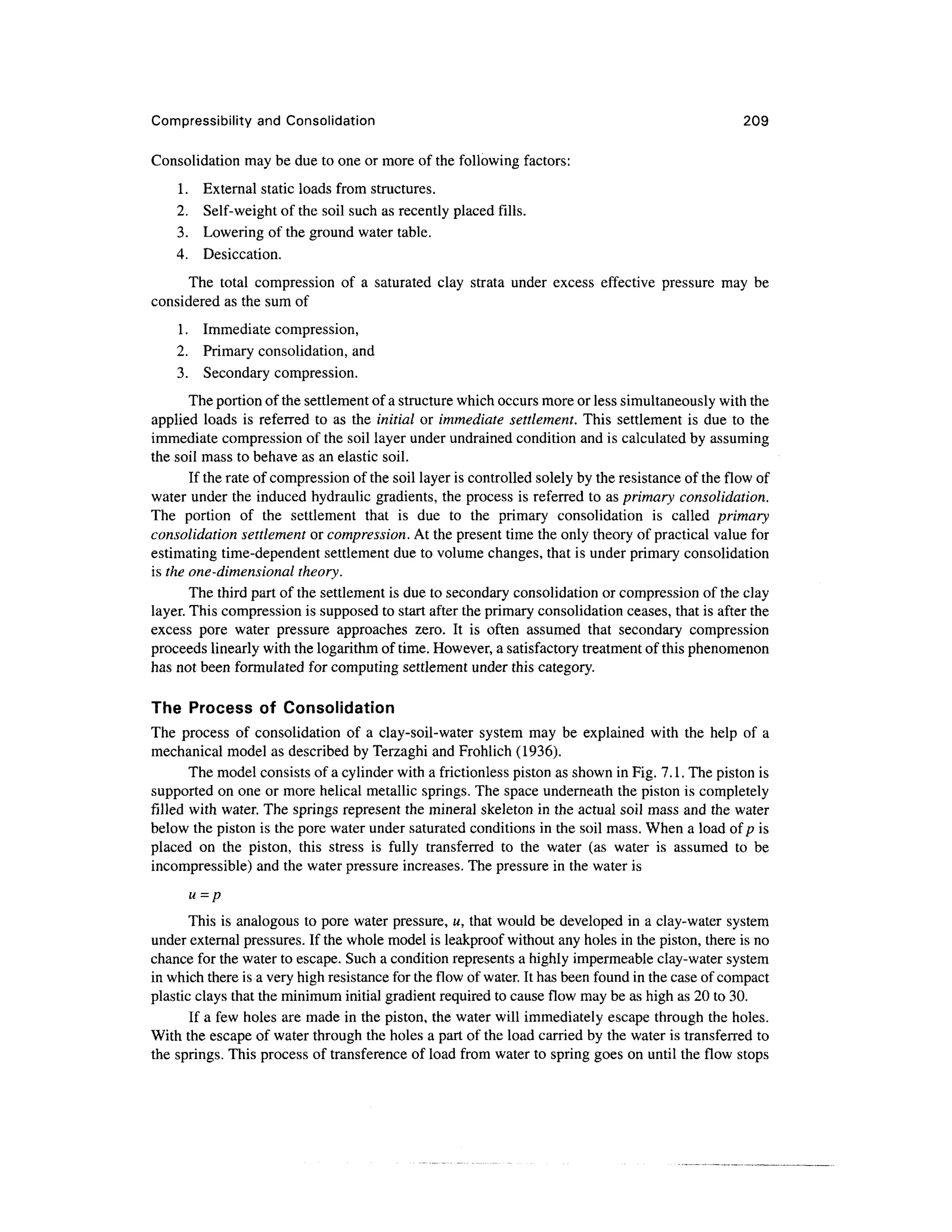
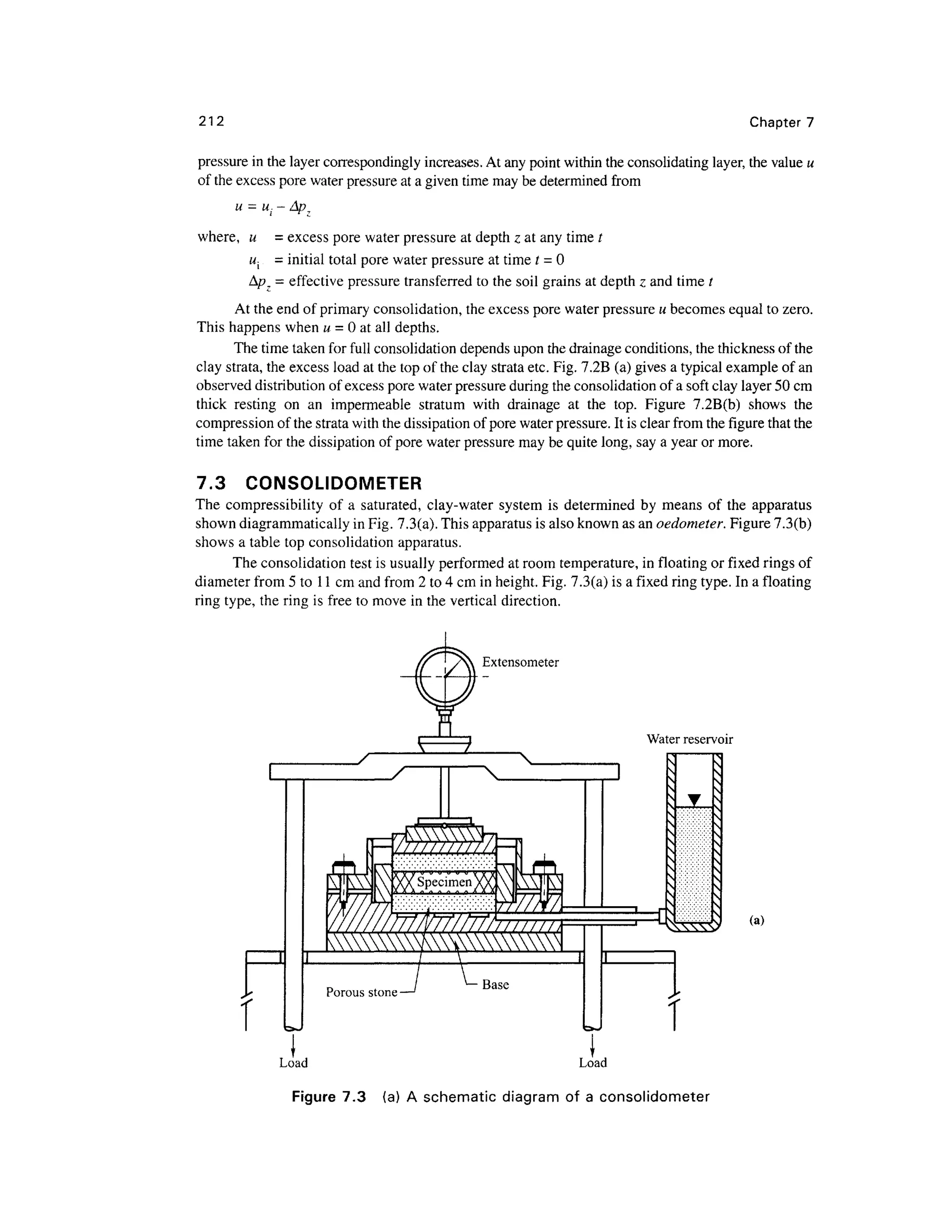
This document provides an overview of soil compressibility and consolidation. It defines consolidation as the process by which saturated clay compresses over time as water drains out of the soil mass and load is gradually transferred from pore water to the soil skeleton. A key aspect of consolidation discussed is the one-dimensional consolidation theory, which models clay layers constrained laterally between impermeable boundaries. The document also describes the consolidometer test apparatus used to measure a soil's compressibility properties and generate pressure-void ratio curves through standardized loading and unloading steps.


![Compressibility and Consolidation 219
7.7 e-log p FIELD CURVES FOR NORMALLY CONSOLIDATED AND
OVERCONSOLIDATED CLAYS OF LOW TO MEDIUM SENSITIVITY
It has been explained earlier with reference to Fig. 7.5, that the laboratory e-log p curve of an
undisturbed sample does not pass through point A and always passes below the point. It has been
found from investigation that the inclined straight portion of e-log p curves of undisturbed or
remolded samples of clay soil intersect at one point at a low void ratio and corresponds to 0.4eQ
shown as point C in Fig. 7.9 (Schmertmann, 1955). It is logical to assume the field curve labelled as
Kf should also pass through this point. The field curve can be drawn from point A, having
coordinates (eQ, /?0), which corresponds to the in-situ condition of the soil. The straight line AC in
Fig. 7.9(a) gives the field curve AT,for normally consolidated clay soil of low sensitivity.
The field curve for overconsolidated clay soil consists of two straight lines, represented by
AB and BC in Fig. 7.9(b). Schmertmann (1955) has shown that the initial section AB of the field
curve is parallel to the mean slope MNof the rebound laboratory curve. Point B is the intersection
point of the vertical line passing through the preconsolidation pressure pc on the abscissa and the
sloping line AB. Since point C is the intersection of the laboratory compression curve and the
horizontal line at void ratio 0.4eQ, line BC can be drawn. The slope of line MN which is the slope
of the rebound curve is called the swell index Cs.
Clay of High Sensitivity
If the sensitivity St is greater than about 8 [sensitivity is defined as the ratio of unconfmed
compressive strengths of undisturbed and remolded soil samples refer to Eq. (3.50)], then the clay
is said to be highly sensitive. The natural water contents of such clay are more than the liquid
limits. The e-log p curve Ku for an undisturbed sample of such a clay will have the initial
branch almost flat as shown in Fig. 7.9(c), and after this it drops abruptly into a steep segment
indicating there by a structural breakdown of the clay such that a slight increase of pressure
leads to a large decrease in void ratio. The curve then passes through a point of inflection at d
and its slope decreases. If a tangent is drawn at the point of inflection d, it intersects the line
eQA at b. The pressure corresponding to b (pb) is approximately equal to that at which the
structural breakdown takes place. In areas underlain by soft highly sensitive clays, the excess
pressure Ap over the layer should be limited to a fraction of the difference of pressure (pt-p0).
Soil of this type belongs mostly to volcanic regions.
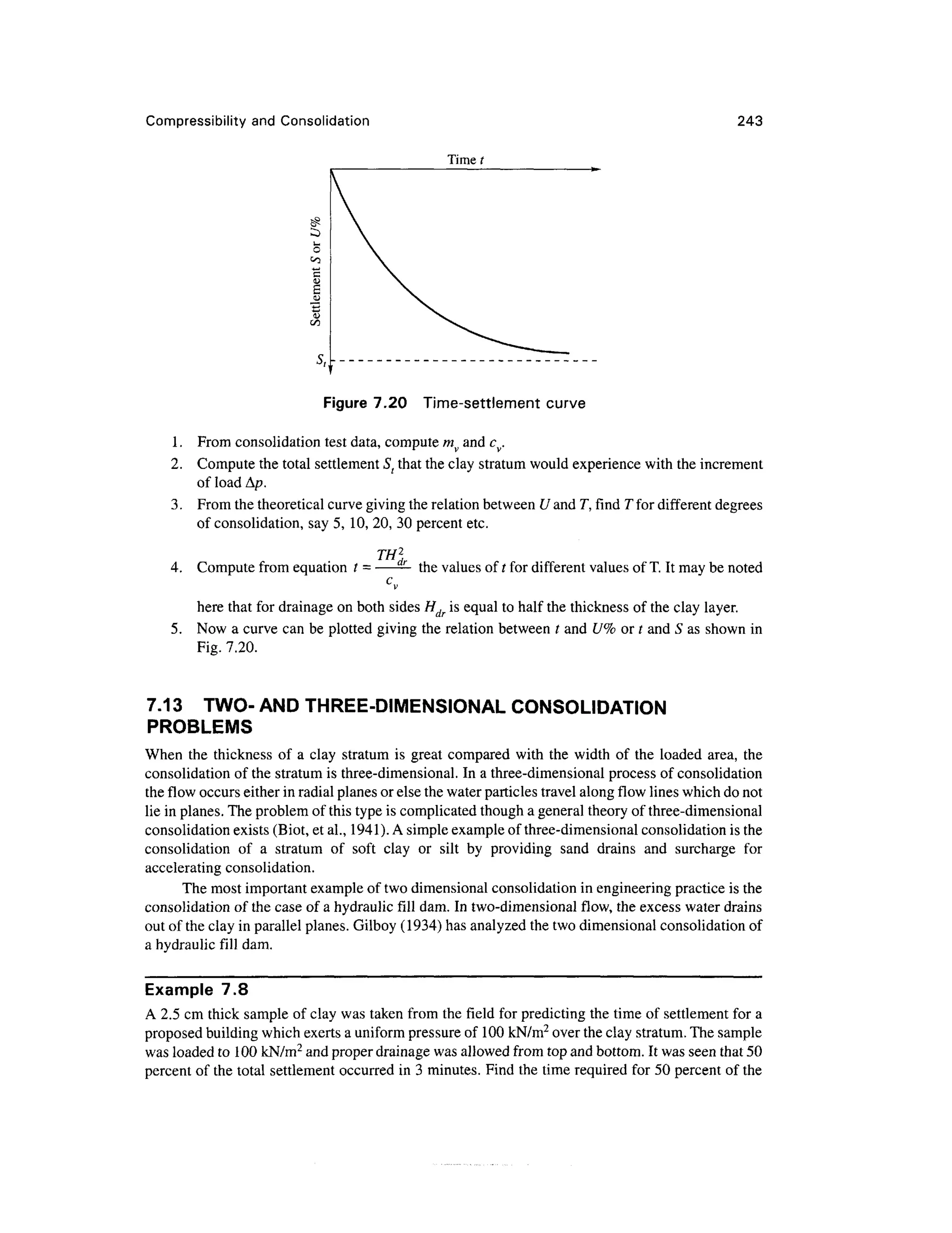
7.8 COMPUTATION OF CONSOLIDATION SETTLEMENT
Settlement Equations for Normally Consolidated Clays
For computing the ultimate settlement of a structure founded on clay the following data are
required
1. The thickness of the clay stratum, H
2. The initial void ratio, eQ
3. The consolidation pressure pQ or pc
4. The field consolidation curve K,
The slope of the field curve K.on a semilogarithmic diagram is designated as the compression
index Cc (Fig. 7.9)
The equation for Cc may be written as
C e
°~e e
°~e Ag
Iogp-logp0 logp/Po logp/pQ
(7
'4)](https://image.slidesharecdn.com/chapter07-220128191204/75/Chapter-07-13-2048.jpg)


![Compressibility and Consolidation 223
Settlement Calculation from e-log p Curve for Overconsolidated Clay Soil
Fig. 7.9(b) gives the field curve Kffor preconsolidated clay soil. The settlement calculation depends
upon the excess foundation pressure Ap over and above the existing overburden pressure pQ.
Settlement Computation, if pQ + A/0 < pc (Fig. 7.9(b))
In such a case, use the sloping line AB. If Cs = slope of this line (also called the swell index), we
have
a
c =
log(p
o+Ap)
(7.14a)
Po
or A* = C,log^ (7.14b)
By substitutingfor A<? in Eq. (7.8), we have
(7.15a)
Settlement Computation, if p0 < pc < p0 + Ap
We may write from Fig.7.9(b)
Pc
(715b)
In this case the slope of both the lines AB and EC in Fig.7.9(b) are required to be considered.
Now the equation for St may be written as [from Eq. (7.8) and Eq. (7.15b)]
CSH pc CCH
log— + —-— log
* Pc
The swell index Cs « 1/5 to 1/10Cc can be used as a check.
Nagaraj and Murthy (1985) have proposed the following equation for Cs as
C =0.0463 -^- G
100 s
where wl = liquid limit, Gs = specific gravity of solids.
Compression Index Cc —Empirical Relationships
Research workers in different parts of the world have established empirical relationships between
the compression index C and other soil parameters. A few of the important relationships are given
below.
Skempton's Formula
Skempton (1944) established a relationship between C, and liquid limits for remolded clays as
Cc =0.007 (wl - 10) (7.16)
where wl is in percent.](https://image.slidesharecdn.com/chapter07-220128191204/75/Chapter-07-17-2048.jpg)


![Compressibility and Consolidation 229
Solution
Per Eq. (7.7), the compression of the fill may be calculated as
where AH = the compression, Ae = change in void ratio, eQ =initial void ratio, HQ =thickness of fill.
Substituting, A/f = L0
~0
-8
x 32.8 = 3.28 ft .
Example 7.3
A stratum of normally consolidated clay 7 m thick is located at a depth 12m below ground level.
The natural moisture content of the clay is 40.5 per cent and its liquid limit is 48 per cent. The
specific gravity of the solid particles is 2.76. The water table is located at a depth 5 m below ground
surface. The soil is sand above the clay stratum.The submerged unit weight of the sand is 1 1 kN/m3
and the same weighs 18 kN/m3
above the water table. The average increase in pressure at the center
of the clay stratum is 120 kN/m2
due to the weight of a building that will be constructed on the sand
above the clay stratum. Estimate the expected settlement of the structure.
Solution
1. Determination of e and yb for the clay [Fig. Ex. 7.3]
W
=1x2.76x1= 2.76 g
405
W = — x2.76 = 1.118 g
w
100
„
r
vs i
= UI& +2.76 = 3.878 g
W
' 1 Q - J / 3
Y, = - = - = 1-83 g/cm
' 2.118
Yb =(1.83-1) = 0.83 g/cm3
.
2. Determination of overburden pressure pQ
PO =yh
i +Y2h
i +yA °r
P0= 0.83x9.81x3.5 + 11x7 + 18x5 = 195.5 kN/m2
3. Compression index [Eq. 11.17]
Cc = 0.009(w, -10) = 0.009 x (48 -10) = 0.34](https://image.slidesharecdn.com/chapter07-220128191204/75/Chapter-07-23-2048.jpg)


![232 Chapter 7
Solution
For calculating settlement [Eq. (7.15a)]
C pn +A/?
S = —— Hlog^-- where &p = 120 kN/ m2
l +eQ pQ
From Eq. (7.17), Cr = 0.009 (w, - 10)= 0.009(45 - 10)= 0.32
wG
From Eq.(3.14a), eQ = - = wG =0.40 x2.78 =1.11 since S= 1
tJ
Yb, the submerged unit weight of clay, is found as follows
MG.+«.) = 9*1(2.78+ Ul) 3
' ^"t 1 , 1 . 1 1 1
l +eQ l + l.ll
Yb=Y^-Yw =18.1-9.81= 8.28 kN/m3
The effective vertical stress pQ at the mid height of the clay layer is
pQ =4.60 x 17.6 + 6x 10.4 +— x 8.28 = 174.8 kN / m2
_ 0.32x7.60, 174.8 + 120
Now St = - log- = 0.26m = 26 cm
1
1+1.11 174.8
Average settlement = 26 cm.
Example 7.6
A soil sample has a compression index of 0.3. If the void ratio e at a stress of 2940 Ib/ft2
is 0.5,
compute (i) the void ratio if the stress is increased to 4200 Ib/ft2
, and (ii) the settlement of a soil
stratum 13 ft thick.
Solution
Given: Cc =0.3, el =0.50, /?, = 2940 Ib/ft2
, p2 =4200 Ib/ft2
.
(i) Now from Eq. (7.4),
p — p
C i %."-)
C = l
- 2
—
or e2 = e]-c
substituting the known values, we have,
e- = 0.5 - 0.31og - 0.454
2
2940
(ii) The settlement per Eq. (7.10) is
c c
c „, Pi 0.3x13x12, 4200
S = —— //log— = - log- = 4.83m.
pl 1.5 2940](https://image.slidesharecdn.com/chapter07-220128191204/75/Chapter-07-26-2048.jpg)


![Geotechnical Engineering-II [Lec #11: Settlement Computation]](https://cdn.slidesharecdn.com/ss_thumbnails/11-181020124840-thumbnail.jpg?width=640&height=640&fit=bounds)


![Geotechnical Engineering-I [Lec #21: Consolidation Problems]](https://cdn.slidesharecdn.com/ss_thumbnails/21-180924141121-thumbnail.jpg?width=640&height=640&fit=bounds)
![Geotechnical Engineering-II [Lec #23: Rankine Earth Pressure Theory]](https://cdn.slidesharecdn.com/ss_thumbnails/23-181123050516-thumbnail.jpg?width=640&height=640&fit=bounds)


![Geotechnical Engineering-II [Lec #7: Soil Stresses due to External Load]](https://cdn.slidesharecdn.com/ss_thumbnails/7-180930132739-thumbnail.jpg?width=640&height=640&fit=bounds)


![Geotechnical Engineering-I [Lec #18: Consolidation-II]](https://cdn.slidesharecdn.com/ss_thumbnails/18-180924140946-thumbnail.jpg?width=640&height=640&fit=bounds)


![Geotechnical Engineering-II [Lec #9+10: Westergaard Theory]](https://cdn.slidesharecdn.com/ss_thumbnails/9-181020124827-thumbnail.jpg?width=640&height=640&fit=bounds)
![Geotechnical Engineering-II [Lec #15 & 16: Schmertmann Method]](https://cdn.slidesharecdn.com/ss_thumbnails/15-181020124920-thumbnail.jpg?width=640&height=640&fit=bounds)
![Geotechnical Engineering-II [Lec #28: Finite Slope Stability Analysis]](https://cdn.slidesharecdn.com/ss_thumbnails/28-181125070402-thumbnail.jpg?width=640&height=640&fit=bounds)
![Geotechnical Engineering-II [Lec #27: Infinite Slope Stability Analysis]](https://cdn.slidesharecdn.com/ss_thumbnails/27-181125070251-thumbnail.jpg?width=640&height=640&fit=bounds)


![Geotechnical Engineering-I [Lec #17: Consolidation]](https://cdn.slidesharecdn.com/ss_thumbnails/17-180924140731-thumbnail.jpg?width=640&height=640&fit=bounds)