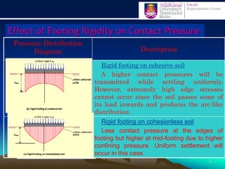
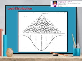
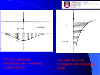
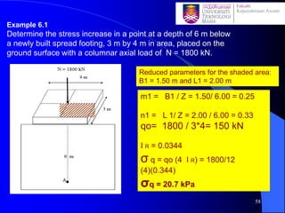
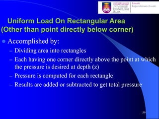
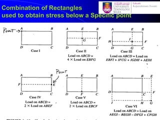
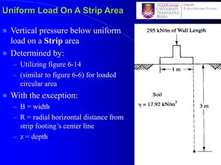
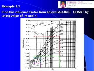
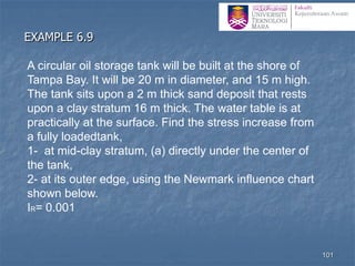
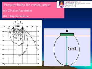
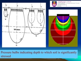
This document discusses stress distribution in soil due to various types of loading. It begins by introducing key concepts like how applied loads are transferred through the soil mass, creating stresses that decrease in magnitude but increase in area with depth. The factors that affect stress distribution, like loading size/shape, soil type, and footing rigidity are also covered. The document then examines specific load types - point loads, line loads, rectangular/triangular strip loads, and circular loads - providing the equations to calculate vertical stress increases below each. Several examples demonstrate calculating stress increases below compound load arrangements. The summary provides an overview of the key topics and calculations presented in the document.


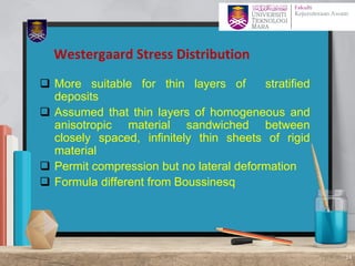
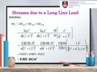
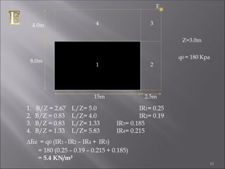
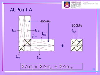
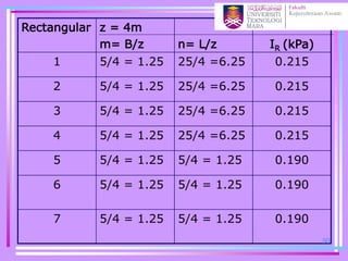
![Σσz = Σσz1 + Σσz2
= q(IR1+IR2+IR3+IR4+IR5- IR6)
+q(4IR7)
= 600[4(0.125) + 0.190 - 0.910]
+ 600[4(0.190)]
= 516 + 456
= 972kPa
91](https://image.slidesharecdn.com/chapter2averticalstress-201031173141/85/Geotechnical-vertical-stress-91-320.jpg)
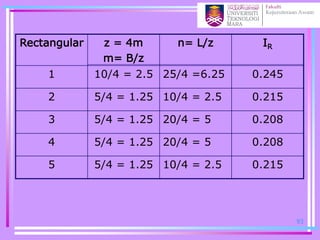
![Σσz = Σσz1 + Σσz2
= q(IR1+IR2+IR3+IR4)+ q(2IR5)
= 600[0.245+0.215+2(0.208)]
+ 600[2(0.215)]
= 525.6 + 258
= 783.6kPa
94](https://image.slidesharecdn.com/chapter2averticalstress-201031173141/85/Geotechnical-vertical-stress-94-320.jpg)
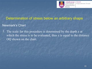
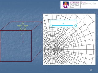
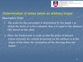
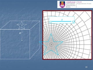
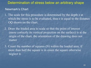
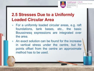
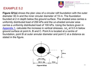
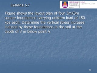
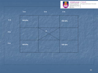
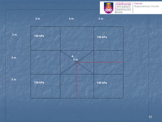
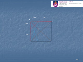
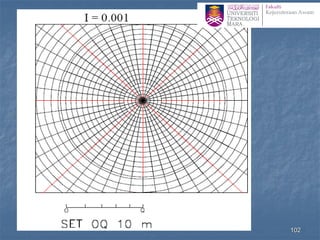
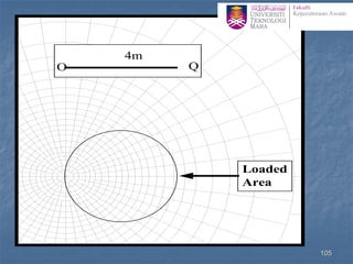
![Determination of stress below an arbitrary shape
Newmark’s Chart
1. The scale for this procedure is determined by the depth z at
which the stress is to be evaluated, thus z is equal to the distance
OQ shown on the chart.
2. Draw the loaded area to scale so that the point of interest
(more correctly its vertical projection on the surface) is at the
origin of the chart, the orientation of the drawing does not
matter
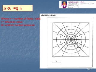
3. Count the number of squares (N) within the loaded area, if
more than half the square is in count the square otherwise
neglect it.
4. The vertical stress increase zz= N ´ [scale factor(0.001)] ´
[surface stress (p)] 100](https://image.slidesharecdn.com/chapter2averticalstress-201031173141/85/Geotechnical-vertical-stress-100-320.jpg)


![Geotechnical Engineering-I [Lec #17: Consolidation]](https://cdn.slidesharecdn.com/ss_thumbnails/17-180924140731-thumbnail.jpg?width=640&height=640&fit=bounds)

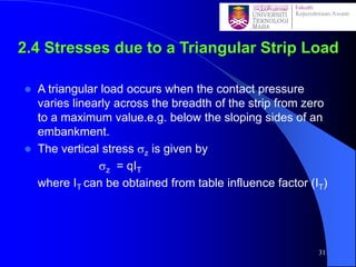
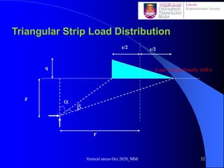
![Geotechnical Engineering-II [Lec #9+10: Westergaard Theory]](https://cdn.slidesharecdn.com/ss_thumbnails/9-181020124827-thumbnail.jpg?width=640&height=640&fit=bounds)

![Geotechnical Engineering-II [Lec #19: General Bearing Capacity Equation]](https://cdn.slidesharecdn.com/ss_thumbnails/19-181123045917-thumbnail.jpg?width=640&height=640&fit=bounds)


![Geotechnical Engineering-II [Lec #13: Elastic Settlements]](https://cdn.slidesharecdn.com/ss_thumbnails/13-181020124852-thumbnail.jpg?width=640&height=640&fit=bounds)

![Geotechnical Engineering-II [Lec #11: Settlement Computation]](https://cdn.slidesharecdn.com/ss_thumbnails/11-181020124840-thumbnail.jpg?width=640&height=640&fit=bounds)


![Geotechnical Engineering-II [Lec #6: Stress Distribution in Soil]](https://cdn.slidesharecdn.com/ss_thumbnails/6-180930132732-thumbnail.jpg?width=640&height=640&fit=bounds)

![Geotechnical Engineering-II [Lec #7: Soil Stresses due to External Load]](https://cdn.slidesharecdn.com/ss_thumbnails/7-180930132739-thumbnail.jpg?width=640&height=640&fit=bounds)
![Geotechnical Engineering-II [Lec #7A: Boussinesq Method]](https://cdn.slidesharecdn.com/ss_thumbnails/7a-181020124807-thumbnail.jpg?width=640&height=640&fit=bounds)


