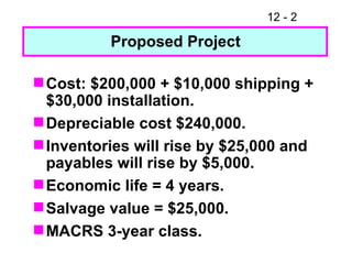
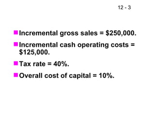
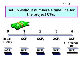
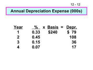
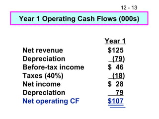
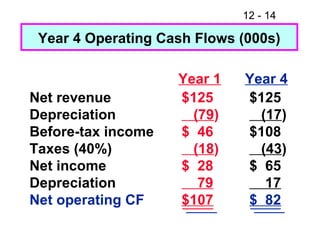
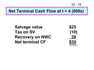
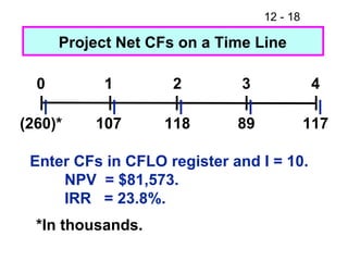
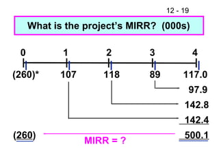
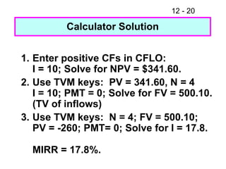
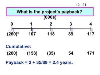
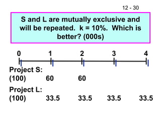
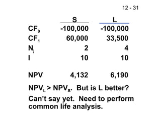
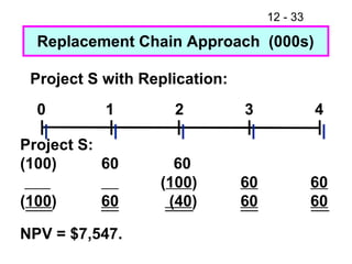
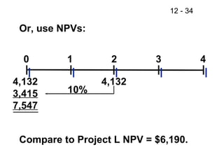
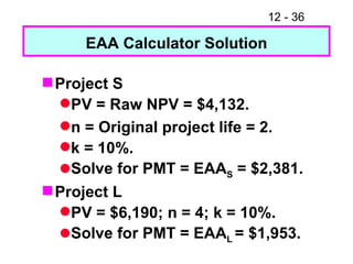
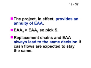
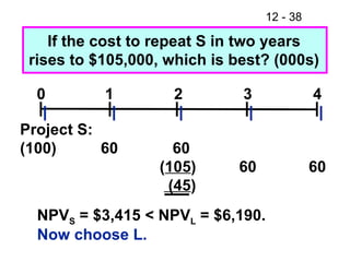
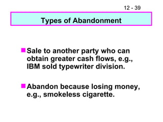
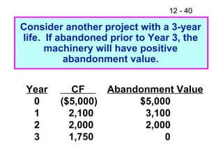
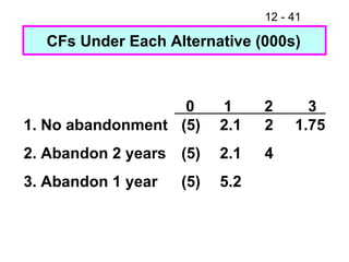
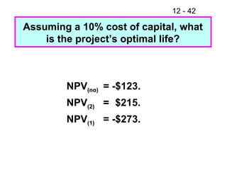
The document discusses concepts related to project cash flow analysis including relevant cash flows, unequal project lives, abandonment value, inflation, and cash flow estimation bias. It provides an example project with initial outlay, operating cash flows, tax rate, salvage value, and cash flows over 4 years. It calculates NPV, IRR, MIRR, and payback for the example project. The document also discusses making decisions between mutually exclusive projects using replacement chains and equivalent annual annuity analysis.

1. Relevant cash flows Working capital treatment Unequal project lives Abandonment value Inflation CHAPTER 12 Project Cash Flow Analysis

2. Cost: $200,000 + $10,000 shipping + $30,000 installation. Depreciable cost $240,000. Inventories will rise by $25,000 and payables will rise by $5,000. Economic life = 4 years. Salvage value = $25,000. MACRS 3-year class. Proposed Project

3. Incremental gross sales = $250,000. Incremental cash operating costs = $125,000. Tax rate = 40%. Overall cost of capital = 10%.

4. 0 1 2 3 4 Initial Outlay OCF 1 OCF 2 OCF 3 OCF 4 + Terminal CF NCF 0 NCF 1 NCF 2 NCF 3 NCF 4 Set up without numbers a time line for the project CFs.

5. = Corporate cash flow with project minus Corporate cash flow without project Incremental Cash Flow

6. NO. The costs of capital are already incorporated in the analysis since we use them in discounting. If we included them as cash flows, we would be double counting capital costs. Should CFs include interest expense? Dividends?

7. NO. This is a sunk cost . Focus on incremental investment and operating cash flows. Suppose $100,000 had been spent last year to improve the production line site. Should this cost be included in the analysis?

8. Yes. Accepting the project means we will not receive the $25,000. This is an opportunity cost and it should be charged to the project. A.T. opportunity cost = $25,000 (1 - T) = $15,000 annual cost. Suppose the plant space could be leased out for $25,000 a year. Would this affect the analysis?

9. Yes. The effects on the other projects’ CFs are “externalities” . Net CF loss per year on other lines would be a cost to this project. Externalities will be positive if new projects are complements to existing assets, negative if substitutes. If the new product line would decrease sales of the firm’s other products by $50,000 per year, would this affect the analysis?

10. Net Investment Outlay at t = 0 (000s) Equipment Freight + Inst. Change in NWC Net CF 0 ($200) (40) (20) ($260)  NWC = $25,000 - $5,000 = $20,000.

11. Basis = Cost + Shipping + Installation $240,000 Depreciation Basics

12. Year 1 2 3 4 % 0.33 0.45 0.15 0.07 Depr. $ 79 108 36 17 x Basis = Annual Depreciation Expense (000s) $240

13. Net revenue Depreciation Before-tax income Taxes (40%) Net income Depreciation Net operating CF $125 (79 ) $ 46 (18 ) $ 28 79 $107 Year 1 Year 1 Operating Cash Flows (000s)

14. Net revenue Depreciation Before-tax income Taxes (40%) Net income Depreciation Net operating CF $125 (79 ) $ 46 (18 ) $ 28 79 $107 $125 (17 ) $108 (43 ) $ 65 17 $ 82 Year 4 Year 1 Year 4 Operating Cash Flows (000s)

15. Net Terminal Cash Flow at t = 4 (000s) Salvage value Tax on SV Recovery on NWC Net terminal CF $25 (10) 20 $35

16. What if you terminate a project before the asset is fully depreciated? Cash flow from sale = Sale proceeds - taxes paid. Taxes are based on difference between sales price and tax basis, where: Basis = Original basis - Accum. deprec.

17. Original basis = $240. After 3 years = $17 remaining. Sales price = $25. Tax on sale = 0.4($25-$17) = $3.2. Cash flow = $25-$3.2=$21.7. Example: If Sold After 3 Years (000s)

18. Project Net CFs on a Time Line Enter CFs in CFLO register and I = 10. NPV = $81,573. IRR = 23.8%. *In thousands. 0 1 2 3 4 (260)* 107 118 89 117

19. What is the project’s MIRR? (000s) ( 260 ) MIRR = ? 0 1 2 3 4 (260)* 107 118 89 117.0 97.9 142.8 142.4 500.1

20. 1. Enter positive CFs in CFLO: I = 10; Solve for NPV = $341.60. 2. Use TVM keys: PV = 341.60, N = 4 I = 10; PMT = 0; Solve for FV = 500.10. (TV of inflows) 3. Use TVM keys: N = 4; FV = 500.10; PV = -260; PMT= 0; Solve for I = 17.8. MIRR = 17.8%. Calculator Solution

21. What is the project’s payback? (000s) Cumulative: Payback = 2 + 35/89 = 2.4 years. 0 1 2 3 4 (260)* (260) 107 (153) 118 (35) 89 54 117 171

22. If this were a replacement rather than a new project, would the analysis change? Yes. The old equipment would be sold and the incremental CFs would be the changes from the old to the new situation.

23. Revenues. Costs. The relevant depreciation would be the change with the new equipment. Also, if the firm sold the old machine now, it would not receive the salvage value at the end of the machine’s life.

24. Coordination with other departments Maintaining consistency of assumptions Elimination of biases in the forecasts What is the role of the financial staff in the cash flow estimation process?

25. CF’s are estimated for many future periods. If company has many projects and errors are random and unbiased, errors will cancel out (aggregate NPV estimate will be OK). Studies show that forecasts often are biased (overly optimistic revenues, underestimated costs). What is cash flow estimation bias?

26. Routinely compare CF estimates with those actually realized and reward managers who are forecasting well, penalize those who are not. When evidence of bias exists, the project’s CF estimates should be lowered or the cost of capital raised to offset the bias. What steps can management take to eliminate the incentives for cash flow estimation bias?

27. Investment in a project may lead to other valuable opportunities. Investment now may extinguish opportunity to undertake same project in the future. True project NPV = NPV + value of options. What is option value?

28. No. Net revenues are assumed to be constant over the 4-year project life, so inflation effects have not been incorporated into the cash flows. If 5% inflation is expected over the next 5 years, are the firm’s cash flow estimates accurate?

29. In DCF analysis, k includes an estimate of inflation. If cash flow estimates are not adjusted for inflation (i.e., are in today’s dollars), this will bias the NPV downward. This bias may offset the optimistic bias of management. Real vs. Nominal Cash flows

30. S and L are mutually exclusive and will be repeated. k = 10%. Which is better? (000s) 0 1 2 3 4 Project S: (100) Project L: (100) 60 33.5 60 33.5 33.5 33.5

31. S L CF 0 -100,000 -100,000 CF 1 60,000 33,500 N j 2 4 I 10 10 NPV 4,132 6,190 NPV L > NPV S . But is L better? Can’t say yet. Need to perform common life analysis.

32. Note that Project S could be repeated after 2 years to generate additional profits. Can use either replacement chain or equivalent annual annuity analysis to make decision.

33. Project S with Replication: NPV = $7,547. Replacement Chain Approach (000s) 0 1 2 3 4 Project S: (100) ( 100 ) 60 60 60 ( 100 ) (40 ) 60 60 60 60

34. Compare to Project L NPV = $6,190. Or, use NPVs: 0 1 2 3 4 4,132 3,415 7,547 4,132 10%

35. Equivalent Annual Annuity (EAA) Approach Finds the constant annuity payment whose PV is equal to the project’s raw NPV over its original life.

36. EAA Calculator Solution Project S PV = Raw NPV = $4,132. n = Original project life = 2. k = 10%. Solve for PMT = EAA S = $2,381. Project L PV = $6,190; n = 4; k = 10%. Solve for PMT = EAA L = $1,953.

37. The project, in effect, provides an annuity of EAA . EAA S > EAA L so pick S. Replacement chains and EAA always lead to the same decision if cash flows are expected to stay the same.

38. If the cost to repeat S in two years rises to $105,000, which is best? (000s) NPV S = $3,415 < NPV L = $6,190. Now choose L. 0 1 2 3 4 Project S: (100) 60 60 ( 105 ) (45 ) 60 60

39. Types of Abandonment Sale to another party who can obtain greater cash flows, e.g., IBM sold typewriter division. Abandon because losing money, e.g., smokeless cigarette.

40. Year 0 1 2 3 CF ($5,000) 2,100 2,000 1,750 Abandonment Value $5,000 3,100 2,000 0 Consider another project with a 3-year life. If abandoned prior to Year 3, the machinery will have positive abandonment value.

41. 1.75 1. No abandonment 2. Abandon 2 years 3. Abandon 1 year (5) (5) (5) 2.1 2.1 5.2 2 4 0 1 2 3 CFs Under Each Alternative (000s)

42. NPV (no) = -$123. NPV (2) = $215. NPV (1) = -$273. Assuming a 10% cost of capital, what is the project’s optimal life?

43. The project is acceptable only if operated for 2 years . A project’s engineering life does not always equal its economic life. The ability to abandon a project may make an otherwise unattractive project acceptable. Abandonment possibilities will be very important when we get to risk. Conclusions