bvcbcnn bn

1. By
By:
:
Prof
Prof.
. Saad Abdel-Hamid Abdel-Hamid Metawa
Saad Abdel-Hamid Abdel-Hamid Metawa
(
(Full Professor of Investment & Finance
Full Professor of Investment & Finance)
)
(
(Faculty of Commerce
Faculty of Commerce -
- Mansoura University)
Mansoura University))
)
2021
2021
Chapter 11
Chapter 11
Cash Flow Estimation and Risk Analysis
Cash Flow Estimation and Risk Analysis

2. • Estimating cash flows:
Estimating cash flows:
• Relevant cash flows
Relevant cash flows
• Working capital treatment
Working capital treatment
• Inflation
Inflation
• Risk Analysis: Sensitivity Analysis, Scenario
Risk Analysis: Sensitivity Analysis, Scenario
Analysis, and Simulation Analysis
Analysis, and Simulation Analysis

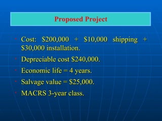
3. • Cost: $200,000 + $10,000 shipping +
Cost: $200,000 + $10,000 shipping +
$30,000 installation.
$30,000 installation.
• Depreciable cost $240,000.
Depreciable cost $240,000.
• Economic life = 4 years.
Economic life = 4 years.
• Salvage value = $25,000.
Salvage value = $25,000.
• MACRS 3-year class.
MACRS 3-year class.
Proposed Project

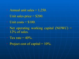
4. • Annual unit sales = 1,250.
Annual unit sales = 1,250.
• Unit sales price = $200.
Unit sales price = $200.
• Unit costs = $100.
Unit costs = $100.
• Net operating working capital (NOWC) =
Net operating working capital (NOWC) =
12% of sales.
12% of sales.
• Tax rate = 40%.
Tax rate = 40%.
• Project cost of capital = 10%.
Project cost of capital = 10%.

5. Incremental Cash Flow for a
Incremental Cash Flow for a
Project
Project
• Project’s incremental cash flow is:
Project’s incremental cash flow is:
• Corporate cash flow
Corporate cash flow with
with the project
the project
• Minus
Minus
• Corporate cash flow
Corporate cash flow without
without the project.
the project.

6. • NO
NO.
. We discount project cash flows with a
We discount project cash flows with a
cost of capital that is the rate of return required by
cost of capital that is the rate of return required by
all investors (not just debtholders or
all investors (not just debtholders or
stockholders), and so we should discount the total
stockholders), and so we should discount the total
amount of cash flow available to all investors.
amount of cash flow available to all investors.
• They are part of the costs of capital. If we
They are part of the costs of capital. If we
subtracted them from cash flows, we would be
subtracted them from cash flows, we would be
double counting capital costs.
double counting capital costs.
Should you subtract interest expense or
dividends when calculating CF?

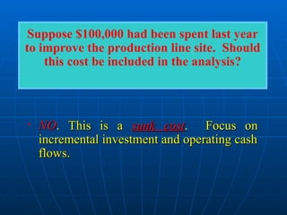
7. • NO
NO. This is a
. This is a sunk cost
sunk cost. Focus on
. Focus on
incremental investment and operating cash
incremental investment and operating cash
flows.
flows.
Suppose $100,000 had been spent last year
to improve the production line site. Should
this cost be included in the analysis?

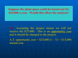
8. • Yes
Yes. Accepting the project means we will not
. Accepting the project means we will not
receive the $25,000. This is an
receive the $25,000. This is an opportunity cost
opportunity cost
and it should be charged to the project.
and it should be charged to the project.
• A.T. opportunity cost = $25,000 (1 - T) = $15,000
A.T. opportunity cost = $25,000 (1 - T) = $15,000
annual cost.
annual cost.
Suppose the plant space could be leased out for
$25,000 a year. Would this affect the analysis?

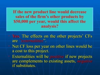
9. • Yes
Yes. The effects on the other projects’ CFs
. The effects on the other projects’ CFs
are
are “externalities
“externalities”.
”.
• Net CF loss per year on other lines would be
Net CF loss per year on other lines would be
a cost to this project.
a cost to this project.
• Externalities will be
Externalities will be positive
positive if new projects
if new projects
are complements to existing assets,
are complements to existing assets, negative
negative
if substitutes.
if substitutes.
If the new product line would decrease
sales of the firm’s other products by
$50,000 per year, would this affect the
analysis?

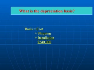
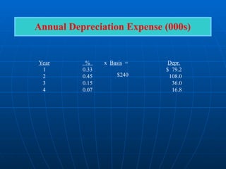
10. Basis = Cost
+ Shipping
+ Installation
$240,000
What is the depreciation basis?

11. Year
1
2
3
4
%
0.33
0.45
0.15
0.07
Depr.
$ 79.2
108.0
36.0
16.8
x Basis =
Annual Depreciation Expense (000s)
$240

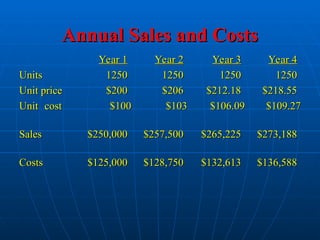
12. Annual Sales and Costs
Annual Sales and Costs
Year 1
Year 1 Year 2
Year 2 Year 3
Year 3 Year 4
Year 4
Units
Units 1250
1250 1250
1250 1250
1250 1250
1250
Unit price
Unit price $200
$200 $206
$206 $212.18
$212.18 $218.55
$218.55
Unit cost
Unit cost $100
$100 $103
$103 $106.09
$106.09 $109.27
$109.27
Sales
Sales $250,000
$250,000 $257,500
$257,500 $265,225
$265,225 $273,188
$273,188
Costs
Costs $125,000
$125,000 $128,750
$128,750 $132,613
$132,613 $136,588
$136,588

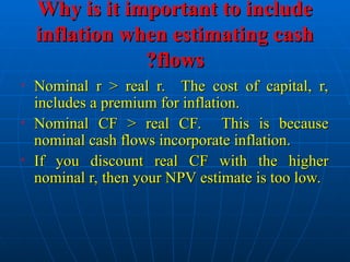
13. Why is it important to include
Why is it important to include
inflation when estimating cash
inflation when estimating cash
flows
flows
?
?
• Nominal r > real r. The cost of capital, r,
Nominal r > real r. The cost of capital, r,
includes a premium for inflation.
includes a premium for inflation.
• Nominal CF > real CF. This is because
Nominal CF > real CF. This is because
nominal cash flows incorporate inflation.
nominal cash flows incorporate inflation.
• If you discount real CF with the higher
If you discount real CF with the higher
nominal r, then your NPV estimate is too low.
nominal r, then your NPV estimate is too low.

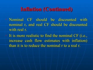
14. Inflation (Continued)
Inflation (Continued)
• Nominal CF should be discounted with
Nominal CF should be discounted with
nominal r, and real CF should be discounted
nominal r, and real CF should be discounted
with real r.
with real r.
• It is more realistic to find the nominal CF (i.e.,
It is more realistic to find the nominal CF (i.e.,
increase cash flow estimates with inflation)
increase cash flow estimates with inflation)
than it is to reduce the nominal r to a real r.
than it is to reduce the nominal r to a real r.

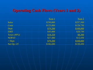
15. Operating Cash Flows (Years 1 and 2)
Operating Cash Flows (Years 1 and 2)
Year 1
Year 1 Year 2
Year 2
Sales
Sales $250,000
$250,000 $257,500
$257,500
Costs
Costs $125,000
$125,000 $128,750
$128,750
Depr.
Depr. $79,200
$79,200 $108,000
$108,000
EBIT
EBIT $45,800
$45,800 $20,750
$20,750
Taxes (40%)
Taxes (40%) $18,320
$18,320 $8,300
$8,300
NOPAT
NOPAT $27,480
$27,480 $12,450
$12,450
+ Depr.
+ Depr. $79,200
$79,200 $108,000
$108,000
Net Op. CF
Net Op. CF $106,680
$106,680 $120,450
$120,450

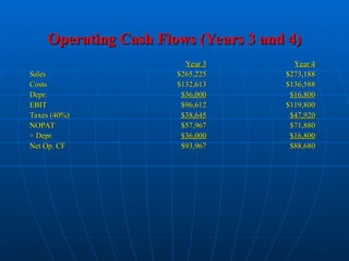
16. Operating Cash Flows (Years 3 and 4)
Operating Cash Flows (Years 3 and 4)
Year 3
Year 3 Year 4
Year 4
Sales
Sales $265,225
$265,225 $273,188
$273,188
Costs
Costs $132,613
$132,613 $136,588
$136,588
Depr.
Depr. $36,000
$36,000 $16,800
$16,800
EBIT
EBIT $96,612
$96,612 $119,800
$119,800
Taxes (40%)
Taxes (40%) $38,645
$38,645 $47,920
$47,920
NOPAT
NOPAT $57,967
$57,967 $71,880
$71,880
+ Depr.
+ Depr. $36,000
$36,000 $16,800
$16,800
Net Op. CF
Net Op. CF $93,967
$93,967 $88,680
$88,680

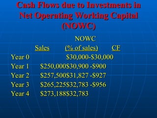
17. Cash Flows due to Investments in
Cash Flows due to Investments in
Net Operating Working Capital
Net Operating Working Capital
(NOWC)
(NOWC)
NOWC
NOWC
Sales
Sales (% of sales)
(% of sales) CF
CF
Year 0
Year 0 $30,000
$30,000-$30,000
-$30,000
Year 1
Year 1 $250,000
$250,000$30,900
$30,900 -$900
-$900
Year 2
Year 2 $257,500
$257,500$31,827
$31,827 -$927
-$927
Year 3
Year 3 $265,225
$265,225$32,783
$32,783 -$956
-$956
Year 4
Year 4 $273,188
$273,188$32,783
$32,783

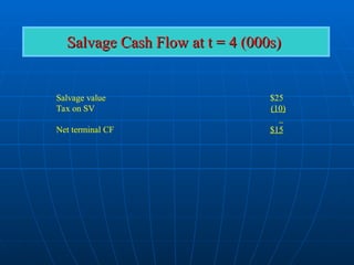
18. Salvage Cash Flow at t = 4 (000s)
Salvage Cash Flow at t = 4 (000s)
Salvage value
Tax on SV
Net terminal CF
$25
(10)
$15

19. What if you terminate a
What if you terminate a
project before the asset is fully
project before the asset is fully
depreciated
depreciated
?
?
Cash flow from sale = Sale proceeds
- taxes paid.
Taxes are based on difference between sales price and tax basis, where:
Basis = Original basis - Accum. deprec.

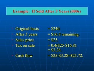
20. • Original basis
Original basis = $240.
= $240.
• After 3 years
After 3 years = $16.8 remaining.
= $16.8 remaining.
• Sales price
Sales price = $25.
= $25.
• Tax on sale
Tax on sale = 0.4($25-$16.8)
= 0.4($25-$16.8)
= $3.28.
= $3.28.
• Cash flow
Cash flow = $25-$3.28=$21.72.
= $25-$3.28=$21.72.
Example: If Sold After 3 Years (000s)

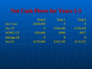
21. Net Cash Flows for Years 1-3
Net Cash Flows for Years 1-3
Year 0
Year 0 Year 1
Year 1 Year 2
Year 2
Init. Cost
Init. Cost -$240,000
-$240,000 0
0 0
0
Op. CF
Op. CF 0
0 $106,680
$106,680 $120,450
$120,450
NOWC CF
NOWC CF -$30,000
-$30,000 -$900
-$900 -$927
-$927
Salvage CF
Salvage CF 0
0 0
0 0
0
Net CF
Net CF -$270,000
-$270,000 $105,780
$105,780 $119,523
$119,523

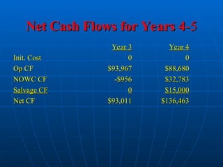
22. Net Cash Flows for Years 4
Net Cash Flows for Years 4-5
-5
Year 3
Year 3 Year 4
Year 4
Init. Cost
Init. Cost 0
0 0
0
Op CF
Op CF $93,967
$93,967 $88,680
$88,680
NOWC CF
NOWC CF -$956
-$956 $32,783
$32,783
Salvage CF
Salvage CF 0
0 $15,000
$15,000
Net CF
Net CF $93,011
$93,011 $136,463
$136,463

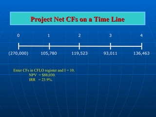
23. Project Net CFs on a Time Line
Project Net CFs on a Time Line
Enter CFs in CFLO register and I = 10.
NPV = $88,030.
IRR = 23.9%.
0 1 2 3 4
(270,000) 105,780 119,523 93,011 136,463

24. What is the project’s MIRR? (000s)
What is the project’s MIRR? (000s)
(270,000)
MIRR = ?
0 1 2 3 4
(270,000) 105,780 119,523 93,011
136,463
102,312
144,623
140,793
524,191

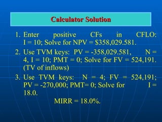
25. 1. Enter positive CFs in CFLO:
I = 10; Solve for NPV = $358,029.581.
2. Use TVM keys: PV = -358,029.581, N =
4, I = 10; PMT = 0; Solve for FV = 524,191.
(TV of inflows)
3. Use TVM keys: N = 4; FV = 524,191;
PV = -270,000; PMT= 0; Solve for I =
18.0.
MIRR = 18.0%.
Calculator Solution
Calculator Solution

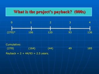
26. What is the project’s payback? (000s)
What is the project’s payback? (000s)
Cumulative:
Payback = 2 + 44/93 = 2.5 years.
0 1 2 3 4
(270)*
(270)
106
(164)
120
(44)
93
49
136
185

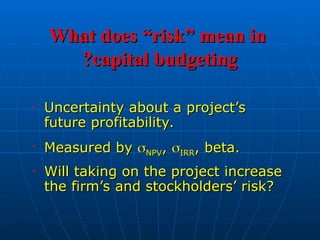
27. What does “risk” mean in
What does “risk” mean in
capital budgeting
capital budgeting
?
?
• Uncertainty about a project’s
Uncertainty about a project’s
future profitability.
future profitability.
• Measured by
Measured by 
NPV
NPV,
, 
IRR
IRR, beta.
, beta.
• Will taking on the project increase
Will taking on the project increase
the firm’s and stockholders’ risk?
the firm’s and stockholders’ risk?

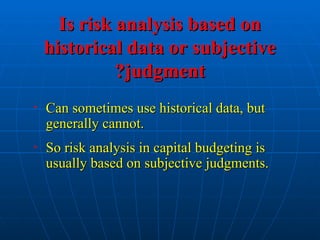
28. Is risk analysis based on
Is risk analysis based on
historical data or subjective
historical data or subjective
judgment
judgment
?
?
• Can sometimes use historical data, but
Can sometimes use historical data, but
generally cannot.
generally cannot.
• So risk analysis in capital budgeting is
So risk analysis in capital budgeting is
usually based on subjective judgments.
usually based on subjective judgments.

29. What three types of risk are
What three types of risk are
relevant in capital budgeting
relevant in capital budgeting
?
?
• Stand-alone risk
Stand-alone risk
• Corporate risk
Corporate risk
• Market (or beta) risk
Market (or beta) risk

30. How is each type of risk measured, and how
How is each type of risk measured, and how
do they relate to one another
do they relate to one another
?
?
1.
1. Stand-Alone Risk
Stand-Alone Risk:
:
• The project’s risk if it were the firm’s only asset
The project’s risk if it were the firm’s only asset
and there were no shareholders.
and there were no shareholders.
• Ignores both firm and shareholder diversification.
Ignores both firm and shareholder diversification.
• Measured by the
Measured by the  or CV of NPV, IRR, or
or CV of NPV, IRR, or
MIRR.
MIRR.

31. 0 E(NPV)
Probability Density
Flatter distribution,
larger , larger
stand-alone risk.
Such graphics are increasingly used
by corporations.
NPV

32. 2.
2. Corporate Risk
Corporate Risk:
:
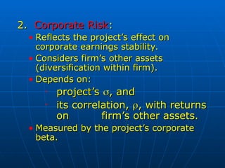
• Reflects the project’s effect on
Reflects the project’s effect on
corporate earnings stability.
corporate earnings stability.
• Considers firm’s other assets
Considers firm’s other assets
(diversification within firm).
(diversification within firm).
• Depends on:
Depends on:
• project’s
project’s 
, and
, and
• its correlation,
its correlation, 
, with returns
, with returns
on
on firm’s other assets.
firm’s other assets.
• Measured by the project’s corporate
Measured by the project’s corporate
beta.
beta.

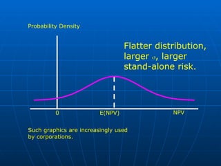
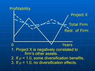
33. Profitability
0 Years
Project X
Total Firm
Rest of Firm
1. Project X is negatively correlated to
firm’s other assets.
2. If  < 1.0, some diversification benefits.
3. If  = 1.0, no diversification effects.

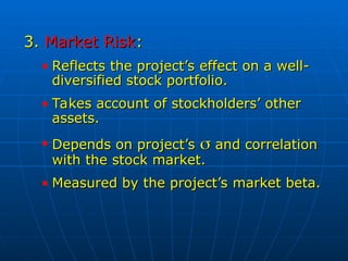
34. 3.
3. Market Risk
Market Risk:
:
• Reflects the project’s effect on a well-
Reflects the project’s effect on a well-
diversified stock portfolio.
diversified stock portfolio.
• Takes account of stockholders’ other
Takes account of stockholders’ other
assets.
assets.
• Depends on project’s
Depends on project’s 
 and correlation
and correlation
with the stock market.
with the stock market.
• Measured by the project’s market beta.
Measured by the project’s market beta.

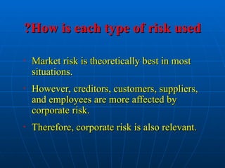
35. How is each type of risk used
How is each type of risk used
?
?
• Market risk is theoretically best in most
Market risk is theoretically best in most
situations.
situations.
• However, creditors, customers, suppliers,
However, creditors, customers, suppliers,
and employees are more affected by
and employees are more affected by
corporate risk.
corporate risk.
• Therefore, corporate risk is also relevant.
Therefore, corporate risk is also relevant.

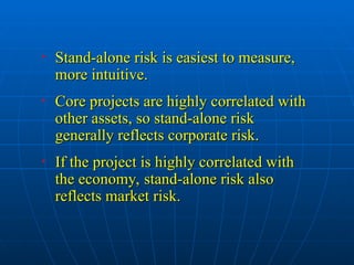
36. • Stand-alone risk is easiest to measure,
Stand-alone risk is easiest to measure,
more intuitive.
more intuitive.
• Core projects are highly correlated with
Core projects are highly correlated with
other assets, so stand-alone risk
other assets, so stand-alone risk
generally reflects corporate risk.
generally reflects corporate risk.
• If the project is highly correlated with
If the project is highly correlated with
the economy, stand-alone risk also
the economy, stand-alone risk also
reflects market risk.
reflects market risk.

37. What is sensitivity analysis
What is sensitivity analysis
?
?
• Shows how changes in a variable such
Shows how changes in a variable such
as unit sales affect NPV or IRR.
as unit sales affect NPV or IRR.
• Each variable is fixed except one.
Each variable is fixed except one.
Change this one variable to see the
Change this one variable to see the
effect on NPV or IRR.
effect on NPV or IRR.
• Answers “what if” questions, e.g. “What
Answers “what if” questions, e.g. “What
if sales decline by 30%?”
if sales decline by 30%?”

38. Sensitivity Analysis
Sensitivity Analysis
-
-
30%
30%
$113
$113
$17
$17
$85
$85
-
-
15%
15%
$100
$100
$52
$52
$86
$86
0%
0%
$88
$88
$88
$88
$88
$88
15%
15%
$76
$76
$124
$124
$90
$90
30%
30%
$65
$65
$159
$159
$91
$91
Change from Resulting NPV (000s)
Base Level r Unit Sales Salvage

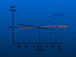
39. -30 -20 -10 Base 10 20 30
Value (%)
88
NPV
(000s)
Unit Sales
Salvage
r

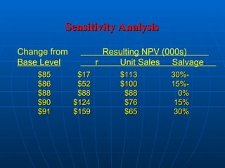
40. Results of Sensitivity Analysis
Results of Sensitivity Analysis
• Steeper sensitivity lines show greater risk.
Steeper sensitivity lines show greater risk.
Small changes result in large declines in NPV.
Small changes result in large declines in NPV.
• Unit sales line is steeper than salvage value or
Unit sales line is steeper than salvage value or
r, so for this project, should worry most about
r, so for this project, should worry most about
accuracy of sales forecast.
accuracy of sales forecast.

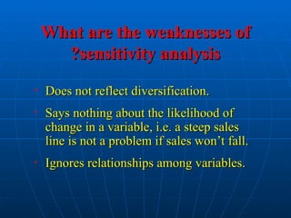
41. What are the weaknesses of
What are the weaknesses of
sensitivity analysis
sensitivity analysis
?
?
• Does not reflect diversification.
Does not reflect diversification.
• Says nothing about the likelihood of
Says nothing about the likelihood of
change in a variable, i.e. a steep sales
change in a variable, i.e. a steep sales
line is not a problem if sales won’t fall.
line is not a problem if sales won’t fall.
• Ignores relationships among variables.
Ignores relationships among variables.

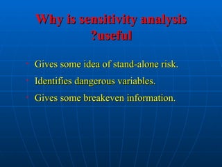
42. Why is sensitivity analysis
Why is sensitivity analysis
useful
useful
?
?
• Gives some idea of stand-alone risk.
Gives some idea of stand-alone risk.
• Identifies dangerous variables.
Identifies dangerous variables.
• Gives some breakeven information.
Gives some breakeven information.

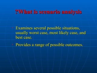
43. What is scenario analysis
What is scenario analysis
?
?
• Examines several possible situations,
Examines several possible situations,
usually worst case, most likely case, and
usually worst case, most likely case, and
best case.
best case.
• Provides a range of possible outcomes.
Provides a range of possible outcomes.

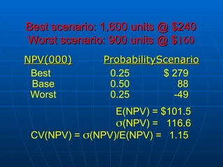
44. Best scenario: 1,600 units @ $240
Best scenario: 1,600 units @ $240
Worst scenario: 900 units @ $
Worst scenario: 900 units @ $160
160
Scenario
Scenario
Probability
Probability
NPV(000)
NPV(000)
Best 0.25 $ 279
Base 0.50 88
Worst 0.25 -49
E(NPV) = $101.5
(NPV) = 116.6
CV(NPV) = (NPV)/E(NPV) = 1.15

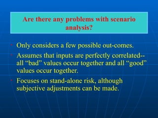
45. Are there any problems with scenario
analysis?
• Only considers a few possible out-comes.
• Assumes that inputs are perfectly correlated--
all “bad” values occur together and all “good”
values occur together.
• Focuses on stand-alone risk, although
subjective adjustments can be made.

46. What is a simulation analysis
What is a simulation analysis
?
?
• A computerized version of scenario analysis
A computerized version of scenario analysis
which uses continuous probability
which uses continuous probability
distributions.
distributions.
• Computer selects values for each variable
Computer selects values for each variable
based on given probability distributions.
based on given probability distributions.

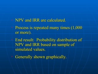
47. • NPV and IRR are calculated.
NPV and IRR are calculated.
• Process is repeated many times (1,000
Process is repeated many times (1,000
or more).
or more).
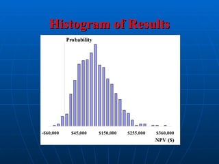
• End result: Probability distribution of
End result: Probability distribution of
NPV and IRR based on sample of
NPV and IRR based on sample of
simulated values.
simulated values.
• Generally shown graphically.
Generally shown graphically.

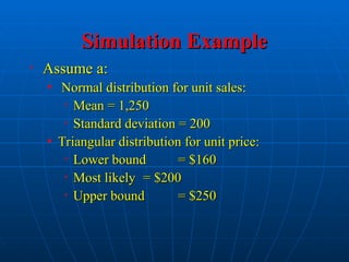
48. Simulation Example
Simulation Example
• Assume a:
Assume a:
• Normal distribution for unit sales:
Normal distribution for unit sales:
• Mean = 1,250
Mean = 1,250
• Standard deviation = 200
Standard deviation = 200
• Triangular distribution for unit price:
Triangular distribution for unit price:
• Lower bound
Lower bound = $160
= $160
• Most likely
Most likely = $200
= $200
• Upper bound
Upper bound = $250
= $250

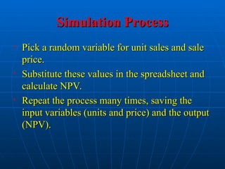
49. Simulation Process
Simulation Process
• Pick a random variable for unit sales and sale
Pick a random variable for unit sales and sale
price.
price.
• Substitute these values in the spreadsheet and
Substitute these values in the spreadsheet and
calculate NPV.
calculate NPV.
• Repeat the process many times, saving the
Repeat the process many times, saving the
input variables (units and price) and the output
input variables (units and price) and the output
(NPV).
(NPV).

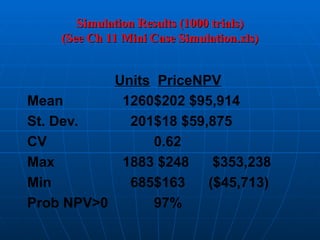
50. Simulation Results (1000 trials)
Simulation Results (1000 trials)
(See Ch 11 Mini Case Simulation.xls)
(See Ch 11 Mini Case Simulation.xls)
Units PriceNPV
Mean 1260$202 $95,914
St. Dev. 201$18 $59,875
CV 0.62
Max 1883 $248 $353,238
Min 685$163 ($45,713)
Prob NPV>0 97%

51. Interpreting the Results
Interpreting the Results
• Inputs are consistent with specificied
Inputs are consistent with specificied
distributions.
distributions.
• Units: Mean = 1260, St. Dev. = 201.
Units: Mean = 1260, St. Dev. = 201.
• Price: Min = $163, Mean = $202, Max = $248.
Price: Min = $163, Mean = $202, Max = $248.
• Mean NPV = $95,914. Low probability of
Mean NPV = $95,914. Low probability of
negative NPV (100% - 97% = 3%).
negative NPV (100% - 97% = 3%).

52. Histogram of Results
Histogram of Results
-$60,000 $45,000 $150,000 $255,000 $360,000
NPV ($)
Probability

53. What are the advantages of
What are the advantages of
simulation analysis
simulation analysis
?
?
• Reflects the probability
Reflects the probability
distributions of each input.
distributions of each input.
• Shows range of NPVs, the
Shows range of NPVs, the
expected NPV,
expected NPV, 
NPV
NPV, and CV
, and CVNPV
NPV.
.
• Gives an intuitive graph of the
Gives an intuitive graph of the
risk situation.
risk situation.

54. What are the disadvantages of
What are the disadvantages of
simulation
simulation
?
?
 Difficult to specify probability distributions
Difficult to specify probability distributions
and correlations.
and correlations.
 If inputs are bad, output will be bad:
If inputs are bad, output will be bad:
“Garbage in, garbage out.”
“Garbage in, garbage out.”

55. • Sensitivity, scenario, and simulation analyses do
Sensitivity, scenario, and simulation analyses do
not provide a decision rule. They do not indicate
not provide a decision rule. They do not indicate
whether a project’s expected return is sufficient to
whether a project’s expected return is sufficient to
compensate for its risk.
compensate for its risk.
• Sensitivity, scenario, and simulation analyses all
Sensitivity, scenario, and simulation analyses all
ignore diversification. Thus they measure only
ignore diversification. Thus they measure only
stand-alone risk, which may not be the most
stand-alone risk, which may not be the most
relevant risk in capital budgeting.
relevant risk in capital budgeting.

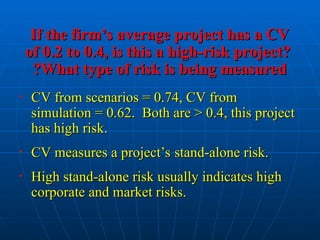
56. If the firm’s average project has a CV
If the firm’s average project has a CV
of 0.2 to 0.4, is this a high-risk project?
of 0.2 to 0.4, is this a high-risk project?
What type of risk is being measured
What type of risk is being measured
?
?
• CV from scenarios = 0.74, CV from
CV from scenarios = 0.74, CV from
simulation = 0.62. Both are > 0.4, this project
simulation = 0.62. Both are > 0.4, this project
has high risk.
has high risk.
• CV measures a project’s stand-alone risk.
CV measures a project’s stand-alone risk.
• High stand-alone risk usually indicates high
High stand-alone risk usually indicates high
corporate and market risks.
corporate and market risks.

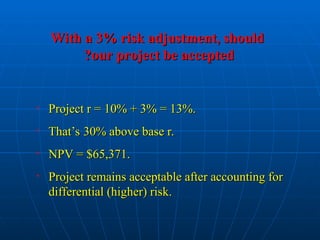
57. With a 3% risk adjustment, should
With a 3% risk adjustment, should
our project be accepted
our project be accepted
?
?
• Project r = 10% + 3% = 13%.
Project r = 10% + 3% = 13%.
• That’s 30% above base r.
That’s 30% above base r.
• NPV = $65,371.
NPV = $65,371.
• Project remains acceptable after accounting for
Project remains acceptable after accounting for
differential (higher) risk.
differential (higher) risk.

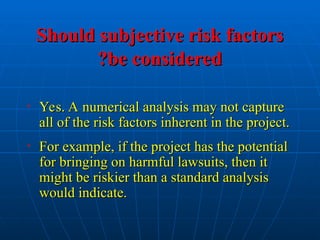
58. Should subjective risk factors
Should subjective risk factors
be considered
be considered
?
?
• Yes. A numerical analysis may not capture
Yes. A numerical analysis may not capture
all of the risk factors inherent in the project.
all of the risk factors inherent in the project.
• For example, if the project has the potential
For example, if the project has the potential
for bringing on harmful lawsuits, then it
for bringing on harmful lawsuits, then it
might be riskier than a standard analysis
might be riskier than a standard analysis
would indicate.
would indicate.