This document provides solutions to practice problems related to capital budgeting techniques and risk analysis. It addresses topics like sunk costs, cash flows, internal rate of return (IRR), modified internal rate of return (MIRR), sensitivity analysis, beta calculation, and risk adjustment. For example, it explains that the MIRR overcomes the unrealistic reinvestment assumption of the IRR method. It also provides steps to estimate a project's beta and discusses using risk-adjusted discount rates for projects with different risk levels.

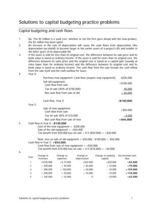
1. Solutions to capital budgeting practice problems
Capital budgeting and cash flows
1. No. The $5 million is a sunk cost: whether or not the firm goes ahead with the new product,
the $5 million has been spent.
2. An increase in the rate of depreciation will cause the cash flows from depreciation (the
depreciation tax-shield) to become larger in the earlier years of a project's life and smaller in
the latter years of its depreciable life.
3. If the asset is sold for less than its original cost, the difference between its sale price and its
book value is taxed as ordinary income. If the asset is sold for more than its original cost, the
difference between its sales price and the original cost is taxed as a capital gain (usually at
rates lower than for ordinary income) and the difference between its original cost and its
book value is taxed as ordinary income. The cash flow from the sale include the cash inflow
from the sale itself and the cash outflow for taxes.
4. Year 0:
Purchase new equipment: Cash flow (acquire new equipment) -$200,000
Sell old equipment:
Cash flow from sale
+$100,000
Tax of sale (40% of $100,000) - 40,000
Net cash flow from sale of old + 60,000
Cash flow, Year 0 -$140,000
Year 5:
Sale of new equipment:
Cash flow from sale
+$50,000
Tax on sale 40% of $10,000 - 4,000
Net cash flow from sale of new +$46,000
5. Cash flow in Year 0: -$130,000
Cost of the new equipment = -$200,000
Sale of the old equipment = +$50,000
Tax benefit from $50,000 loss on sale = 0.4 ($50,000) = +$20,000
Note: loss on sale of old equipment = $50,000 - $100,000 = -$50,000
Cash flow in Year 5: +$54,000
Cash flow from sale of new equipment = +$50,000
Tax benefit from $10,000 loss on sale = 0.4 ($10,000) = +$4,000
6.
Year
Change in
revenues
Change in
expenses
Change in
depreciation
Change in working
capital
Incremental cash
flow
1 +$100,000 +$ 75,000 +$20,000 +$20,000 +$3,500
2 + 200,000 + 90,000 + 40,000 + 10,000 +79,000
3 + 300,000 + 100,000 + 30,000 - 10,000 +159,000
4 + 200,000 + 50,000 + 10,000 - 10,000 +118,000
5 + 100,000 + 25,000 0 - 10,000 +62,500
Solutions to capital budgeting practice problems 1

2. Capital budgeting techniques
1. The internal rate of return on an investment is the return considering the cash inflows and
the reinvestment of the cash inflows (at this IRR). The yield to maturity of a bond is the
return on the bond from interest, the reinvestment of the interest (at this yield), and the
principal repayment.
2. The source of this conflict is the reinvestment rate assumption. The NPV method assumes
reinvestment at the required rate of return, whereas the IRR assumes reinvestment at the
IRR. For certain required rates of return, the project with the higher IRR may not have the
greatest present value.
3. The source of this conflict is the manner in which the method assesses the investment. The
NPV produces a dollar value of wealth enhancement, whereas the IRR is in terms of a yield.
4. The MIRR is designed to overcome the reinvestment rate assumption inherent in the IRR
method. Since the IRR method's reinvestment assumption may be unrealistic, the MIRR
provides an alternative method that permits a more realistic reinvestment assumption to be
built-in.
5.
a. IRR = 15%
b. MIRR = 8.8%
Note: FV = Terminal value = $35,027 x 4 = $140,108
c. MIRR = 12.92%
Because the cash flows are the same, we can use the future value o an annuity to
solve for the terminal value:
FV = Terminal value = $35,027 (FV annuity factor for n=4 i = 10%)
FV = $162,560
6.
a. IRR = 15%
Use the annuity relation to determine the i (the IRR).
b. MIRR = 13.178%
Terminal value = $144,971.38
c. MIRR = 14.6359%
Terminal value = $150,647.60
7.
a. IRR = 18.7189%
b. MIRR = 14.6873%
Terminal value = $396,831.50
c. MIRR = 16.9875%
Terminal value = $438,254.78
8.
a. IRR = 15%
b. MIRR = 15%
Note: Because there is only one cash inflow, you can use the following to solve for
the MIRR: FV = $174,901; PV = $100,000;n = 4; Solve for i (the MIRR)
Solutions to capital budgeting practice problems 2

3. Capital budgeting and risk
1. The standard deviation of the expected value is a measure of dispersion about the expected
value; that is, how the possible outcomes deviate from the central tendency of the probability
distribution. The standard deviation is in the same unit of measure as the expected value
(e.g. dollars, return, units sold). The coefficient of variation is a measure of dispersion that is
standardized to reflect dispersion relative to the expected value (e.g. a coefficient of variation
of 2.0 indicates that the standard deviation is two times the expected value). The coefficient
of variation is useful in comparing the dispersion of distributions that are centered on
different expected values.
2. A standard deviation of $500 and an expected value of $1,200 indicates that it is 64% likely
that the possible outcome will be within 1.64 ($500) or $820 either side of the expected
value of $1,200, or in the range $380 to $2,020. [Note: The 64% and the 1.64 are based on
the properties of the normal distribution.]
3. Procedure:
Step 1: Classify the project in terms of its line of business
Step 2: Identify firms with single lines of business that are the same as the project's, and
whose stock is traded in the financial markets
Step 3: Calculate the beta of the firm's or firms' stock
Step 4: Unlever the betas
Step 5: If there is more than one firm in the same line of business, average their betas
This will produce an estimate of the project's beta.
4. Sensitivity analysis involves modifying one parameter at a time in the examination possible
future outcomes to a decision, whereas simulation analysis allows modifying more than one
parameter and explicitly incorporates the probability distributions of the parameters of the
decision.
5. The approach to determine the cost of capital for a small, single owner business would be
different than that of a large publicly-held corporation since stand-alone, or project specific
risk is more important for the small, single owner firm than for the large corporation. In the
case of large corporation, the focus should be on the project's market risk, not on a project's
total risk.
6. Using a single rate to evaluate all projects is not a problem as long as all projects have the
same risk and this risk is the same as that of the rest of the firm's projects.
If the projects differ in terms of riskiness, a single rate will result in the rejection of
profitable, yet less risky projects and the acceptance of unprofitable projects with risk greater
than the average project's risk.
7. Using risk classes is a step towards using risk-adjusted discount rates. However, there are
two potential problems:
(1) Determining the discount rates for the risk classes
(2) The possibility that projects within a given class will have different risks.
8. Neither. The total risk of the two products is the same (that is, they have identical coefficient
of variations):
Coefficient of variation, Product A = $2/$10 = 0.20
Coefficient of variation, Product B = $3/$15 = 0.20
9.
a. Expected cash flow = $0.2 + $1.2 + 2.0 = $3.40
b. Standard deviation = $1.4967
c. Coefficient of variation = $1.4976/ $3.4000 = 0.4405
10. Calculate the asset beta for each firm, III, JJJ and KKK:
Firm III: 1.5 (0.5714) = 0.8571
Firm JJJ: 1.5 (0.6557) = 0.9836
Firm KKK: 1.0 (0.6250) = 0.6250
Solutions to capital budgeting practice problems 3