Downloaded 722 times


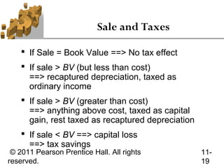
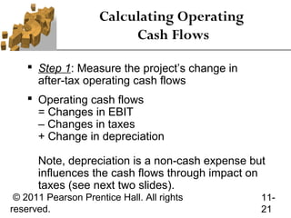
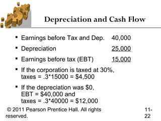
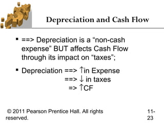
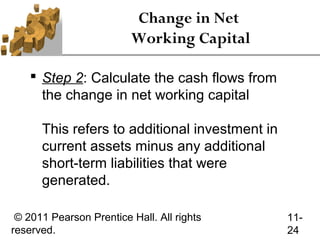
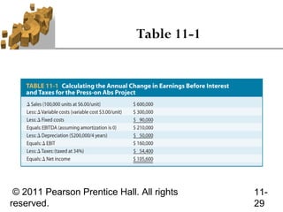
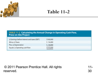
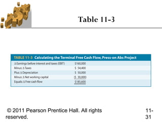
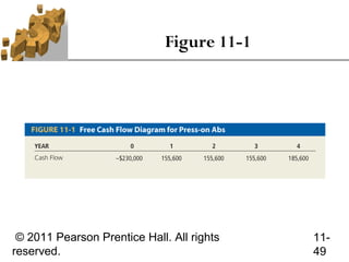

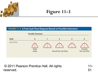
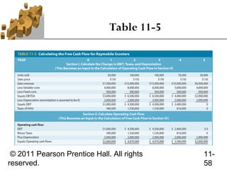
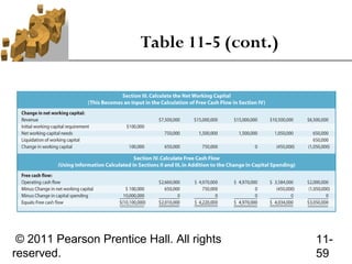

This document discusses guidelines for capital budgeting cash flow analysis. It covers calculating free cash flows, which have three components: initial cash outlay, annual differential cash flows over the project life, and terminal cash flow. Free cash flows consider operating cash flows from changes in earnings before interest and taxes and depreciation, as well as working capital requirements and capital spending. Depreciation is discussed as affecting taxes and thus cash flows, even though it is a non-cash expense. Guidelines for treatment of items like sunk costs, opportunity costs, and overhead costs are provided.