Download free for 30 days
Sign in
Upload
Language (EN)
Support
Business
Mobile
Social Media
Marketing
Technology
Art & Photos
Career
Design
Education
Presentations & Public Speaking
Government & Nonprofit
Healthcare
Internet
Law
Leadership & Management
Automotive
Engineering
Software
Recruiting & HR
Retail
Sales
Services
Science
Small Business & Entrepreneurship
Food
Environment
Economy & Finance
Data & Analytics
Investor Relations
Sports
Spiritual
News & Politics
Travel
Self Improvement
Real Estate
Entertainment & Humor
Health & Medicine
Devices & Hardware
Lifestyle
Change Language
Language
English
Español
Português
Français
Deutsche
Cancel
Save
EN
Uploaded by
MochammadRidwanRisty3
PPT, PDF
8 views
ffm912-cash-flow-estimation-and-risk-analysis.ppt
fm912-cash-flow-estimation-and-risk-analysis
Education
◦
Read more
0
Save
Share
Embed
Embed presentation
Download
Download to read offline
1
/ 39
2
/ 39
3
/ 39
4
/ 39
5
/ 39
6
/ 39
7
/ 39
8
/ 39
9
/ 39
10
/ 39
11
/ 39
12
/ 39
13
/ 39
14
/ 39
15
/ 39
16
/ 39
17
/ 39
18
/ 39
19
/ 39
20
/ 39
21
/ 39
22
/ 39
23
/ 39
24
/ 39
25
/ 39
26
/ 39
27
/ 39
28
/ 39
29
/ 39
30
/ 39
31
/ 39
32
/ 39
33
/ 39
34
/ 39
35
/ 39
36
/ 39
37
/ 39
38
/ 39
39
/ 39
More Related Content
PPT
CashFlow/dsc/LTV/triple net for cash flow
by
Ludwig
PPT
3 aminullah assagaf ch. 11 sd15_financial management_22 okt 2020
by
Aminullah Assagaf
PPT
Aminullah assagaf financial management p1115_ch. 11 sd15_28 mei 2021
by
Aminullah Assagaf
PPT
Aminullah assagaf p1115 ch. 11 sd15_financial management_28 mei 2021
by
Aminullah Assagaf
PPT
Fm11 ch 11 cash flow estimation and risk analysis
by
Nhu Tuyet Tran
PPT
260928092-Cash-Flow-Estimation-and-Risk-Analysis.ppt
by
MochammadRidwanRisty3
DOCX
Cash Flow Estimation and Risk AnalysisCHAPTER 11© 2020 Cenga.docx
by
troutmanboris
DOCX
Cash Flow Estimation and Risk AnalysisCHAPTER 11© 2020 Cenga.docx
by
keturahhazelhurst
CashFlow/dsc/LTV/triple net for cash flow
by
Ludwig
3 aminullah assagaf ch. 11 sd15_financial management_22 okt 2020
by
Aminullah Assagaf
Aminullah assagaf financial management p1115_ch. 11 sd15_28 mei 2021
by
Aminullah Assagaf
Aminullah assagaf p1115 ch. 11 sd15_financial management_28 mei 2021
by
Aminullah Assagaf
Fm11 ch 11 cash flow estimation and risk analysis
by
Nhu Tuyet Tran
260928092-Cash-Flow-Estimation-and-Risk-Analysis.ppt
by
MochammadRidwanRisty3
Cash Flow Estimation and Risk AnalysisCHAPTER 11© 2020 Cenga.docx
by
troutmanboris
Cash Flow Estimation and Risk AnalysisCHAPTER 11© 2020 Cenga.docx
by
keturahhazelhurst
Similar to ffm912-cash-flow-estimation-and-risk-analysis.ppt
PPT
Ch12ppt
by
JESSIEOU
PPT
Capital budgeting cash flow estimation
by
Prafulla Tekriwal
PPT
Cash Flow Estimation.ppt
by
AdiVanIon1
PPT
Chapter 11 - Cash Flow Estimation and Risk Analysis.ppt
by
AhmedElGayar13
PDF
AF3313 - Lecture 4 - accccc Chapter 6.pdf
by
mksellson
PPTX
CAPITAL BUDGETING DISCUSSION FINMAN.pptx
by
catolicojoaennelzhen
PDF
Ch14sol cash flow estimation
by
Hassan Zada
PPT
Chap010
by
Morten Andersen
PPTX
Corporate Finance Chapter (3).pptx ggghg
by
rafidullah1
PDF
Risk Analysis and Project Evaluation/Abshor.Marantika/Gita Mutiara Ovelia/3-3
by
gitaovelia
DOC
Cb practice problems
by
Bathini Hari Babu
PPT
Cff311.ppt
by
Reema975562
PPT
Additional File-Capital Budgeting 3.ppt
by
ArneetSarna1
DOCX
aPart 5 Corporate Valuation and GovernanceEasy Problem.docx
by
justine1simpson78276
DOCX
1. Payback Period and Net Present Value[LO1, 2] If a project with .docx
by
paynetawnya
PPT
Capital budgeting
by
Jaffer Vailankara
PPT
Chapter 9.Risk and Managerial Options in Capital Budgeting
by
ZahraMirzayeva
PPT
Capital Budgeting
by
yashpal01
PDF
Group 2, Presentation, Making Investment Decision (Cash Flow Protection), F.M...
by
JokZemarko
PPTX
Project Profitability Analysis and Evaluation
by
Arpit Amar
Ch12ppt
by
JESSIEOU
Capital budgeting cash flow estimation
by
Prafulla Tekriwal
Cash Flow Estimation.ppt
by
AdiVanIon1
Chapter 11 - Cash Flow Estimation and Risk Analysis.ppt
by
AhmedElGayar13
AF3313 - Lecture 4 - accccc Chapter 6.pdf
by
mksellson
CAPITAL BUDGETING DISCUSSION FINMAN.pptx
by
catolicojoaennelzhen
Ch14sol cash flow estimation
by
Hassan Zada
Chap010
by
Morten Andersen
Corporate Finance Chapter (3).pptx ggghg
by
rafidullah1
Risk Analysis and Project Evaluation/Abshor.Marantika/Gita Mutiara Ovelia/3-3
by
gitaovelia
Cb practice problems
by
Bathini Hari Babu
Cff311.ppt
by
Reema975562
Additional File-Capital Budgeting 3.ppt
by
ArneetSarna1
aPart 5 Corporate Valuation and GovernanceEasy Problem.docx
by
justine1simpson78276
1. Payback Period and Net Present Value[LO1, 2] If a project with .docx
by
paynetawnya
Capital budgeting
by
Jaffer Vailankara
Chapter 9.Risk and Managerial Options in Capital Budgeting
by
ZahraMirzayeva
Capital Budgeting
by
yashpal01
Group 2, Presentation, Making Investment Decision (Cash Flow Protection), F.M...
by
JokZemarko
Project Profitability Analysis and Evaluation
by
Arpit Amar
More from MochammadRidwanRisty3
PPTX
BALANCE SCORECARD konsep perhitungan.pptx
by
MochammadRidwanRisty3
PDF
497231341-Turban-10e-Ppt-Ch12-en-id-1.pdf
by
MochammadRidwanRisty3
PPTX
852592845-Brigham-FFM16-Concise11-Ch14-PPT.pptx
by
MochammadRidwanRisty3
PDF
Model Antrian_Riset Operasi latihan soal.pdf
by
MochammadRidwanRisty3
PPT
ch08 supply chain management and erp.ppt
by
MochammadRidwanRisty3
PPT
ch09 planning and business process redesign.ppt
by
MochammadRidwanRisty3
PPT
235669801-model-antrian-riset operasional.ppt
by
MochammadRidwanRisty3
PPTX
454065865-bab-12-Estimasi-Arus-Kas-dan-Analisis-Risiko-new-pptx.pptx
by
MochammadRidwanRisty3
PPTX
Mengukur dan Mengelola Paparan Terjemahan dan Transaksi.pptx
by
MochammadRidwanRisty3
PPT
ch12 international financial funds and national capital
by
MochammadRidwanRisty3
PPTX
Financial Futures discuss study in class
by
MochammadRidwanRisty3
PPTX
FIN335 CH08 Risk&Return presentation study
by
MochammadRidwanRisty3
PPT
bahan ke-5 produksi dan teori biaya produksi.ppt
by
MochammadRidwanRisty3
PPTX
Biaya dan Estimasi dan perkiraan biaya produksi
by
MochammadRidwanRisty3
PPT
Prestasi Manajemen Keuangan Internasional BAB 9
by
MochammadRidwanRisty3
BALANCE SCORECARD konsep perhitungan.pptx
by
MochammadRidwanRisty3
497231341-Turban-10e-Ppt-Ch12-en-id-1.pdf
by
MochammadRidwanRisty3
852592845-Brigham-FFM16-Concise11-Ch14-PPT.pptx
by
MochammadRidwanRisty3
Model Antrian_Riset Operasi latihan soal.pdf
by
MochammadRidwanRisty3
ch08 supply chain management and erp.ppt
by
MochammadRidwanRisty3
ch09 planning and business process redesign.ppt
by
MochammadRidwanRisty3
235669801-model-antrian-riset operasional.ppt
by
MochammadRidwanRisty3
454065865-bab-12-Estimasi-Arus-Kas-dan-Analisis-Risiko-new-pptx.pptx
by
MochammadRidwanRisty3
Mengukur dan Mengelola Paparan Terjemahan dan Transaksi.pptx
by
MochammadRidwanRisty3
ch12 international financial funds and national capital
by
MochammadRidwanRisty3
Financial Futures discuss study in class
by
MochammadRidwanRisty3
FIN335 CH08 Risk&Return presentation study
by
MochammadRidwanRisty3
bahan ke-5 produksi dan teori biaya produksi.ppt
by
MochammadRidwanRisty3
Biaya dan Estimasi dan perkiraan biaya produksi
by
MochammadRidwanRisty3
Prestasi Manajemen Keuangan Internasional BAB 9
by
MochammadRidwanRisty3
Recently uploaded
PPTX
Unit 3- Culture.pptx....................
by
Akanksha Kotangale
PPTX
Day 2 ppt english.powerpoint presentation ppt
by
JeahMaeMedez
PPTX
"Aristotle : Father Of Western Philosophy"
by
mitalbarathod28
PPTX
literary theory and criticism by Vivek p
by
vivekrathodborda
PDF
Lamarckism: Theory of Evolution, Principles, Examples, Objections and Neo-Lam...
by
IPGDCWA,NAMPALLY
PPTX
PREVENTIVE PEDIATRICS.pptx
by
BANDITA PATRA
PPTX
Appreciations - Jan 26 01.pptxkjkjkkjkjkjkj
by
preetheshparmar
PPTX
" Jaya : Silence as Resistance " - That long silence
by
dharabhandari35
PPTX
West Hatch High School - GCSE Media Studies
by
WestHatch
PPTX
COMMUNICATION ITS PROCESS ELEMENTS & BARRIER .pptx
by
PoojaSen20
PDF
Beak Modifications by Dr. Ramzan Virani pptx.pdf
by
Dr. Ramzan Virani
PDF
Risks and opportunities of artificial intelligence in education: A critical view
by
Yannis
PPTX
Poster Based Ethical Reflection - Dharma and Values Poster.pptx
by
RajshreeBeneymadoo
PDF
Darwinism: Theory of Natural Selection and Origin of Species
by
IPGDCWA,NAMPALLY
PPTX
Metabolism ( BIOCHEMISTRY & CLINICAL PATHOLOGY )
by
BushraDeshpande
PDF
Chapter 05 Drug Acting on CNS Sedatives & Hypnotics | Antipsychotics.pdf
by
SandeshSul
PPTX
Payment Follow-Up via WhatsApp in Odoo 18.1 Accounting
by
Celine George
PDF
Aminoglycosides.pdf for B.Pharmacy Medicinal Chemistry-III (BP601T), GPAT, a...
by
mominzarinamdnajeeb
PPTX
Master of Punjabi Short Story "kartar singh duggal
by
bhautikbharwad4
PPTX
28 January 2026 Rebecca Frankum Are high-stakes exams and assessments still r...
by
EduSkills OECD
Unit 3- Culture.pptx....................
by
Akanksha Kotangale
Day 2 ppt english.powerpoint presentation ppt
by
JeahMaeMedez
"Aristotle : Father Of Western Philosophy"
by
mitalbarathod28
literary theory and criticism by Vivek p
by
vivekrathodborda
Lamarckism: Theory of Evolution, Principles, Examples, Objections and Neo-Lam...
by
IPGDCWA,NAMPALLY
PREVENTIVE PEDIATRICS.pptx
by
BANDITA PATRA
Appreciations - Jan 26 01.pptxkjkjkkjkjkjkj
by
preetheshparmar
" Jaya : Silence as Resistance " - That long silence
by
dharabhandari35
West Hatch High School - GCSE Media Studies
by
WestHatch
COMMUNICATION ITS PROCESS ELEMENTS & BARRIER .pptx
by
PoojaSen20
Beak Modifications by Dr. Ramzan Virani pptx.pdf
by
Dr. Ramzan Virani
Risks and opportunities of artificial intelligence in education: A critical view
by
Yannis
Poster Based Ethical Reflection - Dharma and Values Poster.pptx
by
RajshreeBeneymadoo
Darwinism: Theory of Natural Selection and Origin of Species
by
IPGDCWA,NAMPALLY
Metabolism ( BIOCHEMISTRY & CLINICAL PATHOLOGY )
by
BushraDeshpande
Chapter 05 Drug Acting on CNS Sedatives & Hypnotics | Antipsychotics.pdf
by
SandeshSul
Payment Follow-Up via WhatsApp in Odoo 18.1 Accounting
by
Celine George
Aminoglycosides.pdf for B.Pharmacy Medicinal Chemistry-III (BP601T), GPAT, a...
by
mominzarinamdnajeeb
Master of Punjabi Short Story "kartar singh duggal
by
bhautikbharwad4
28 January 2026 Rebecca Frankum Are high-stakes exams and assessments still r...
by
EduSkills OECD
ffm912-cash-flow-estimation-and-risk-analysis.ppt
1.
12 - 1 Copyright
© 2001 by Harcourt, Inc. All rights reserved. CHAPTER 12 Cash Flow Estimation and Risk Analysis Relevant cash flows Incorporating inflation Types of risk
2.
12 - 2 Copyright
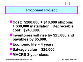
© 2001 by Harcourt, Inc. All rights reserved. Proposed Project Cost: $200,000 + $10,000 shipping + $30,000 installation. Depreciable cost: $240,000. Inventories will rise by $25,000 and payables by $5,000. Economic life = 4 years. Salvage value = $25,000. MACRS 3-year class.
3.
12 - 3 Copyright
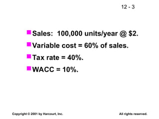
© 2001 by Harcourt, Inc. All rights reserved. Sales: 100,000 units/year @ $2. Variable cost = 60% of sales. Tax rate = 40%. WACC = 10%.
4.
12 - 4 Copyright
© 2001 by Harcourt, Inc. All rights reserved. Set up, without numbers, a time line for the project’s cash flows. 0 1 2 3 4 OCF1 OCF2 OCF3 OCF4 Initial Costs (CF0) + Terminal CF NCF0 NCF1 NCF2 NCF3 NCF4
5.
12 - 5 Copyright
© 2001 by Harcourt, Inc. All rights reserved. Equipment -$200 Installation & Shipping -40 Increase in inventories -25 Increase in A/P 5 Net CF0 -$260 NOWC = $25 – $5 = $20. Investment at t = 0:
6.
12 - 6 Copyright
© 2001 by Harcourt, Inc. All rights reserved. What’s the annual depreciation? Due to 1/2-year convention, a 3-year asset is depreciated over 4 years. Year Rate x Basis Depreciation 1 0.33 $240 $ 79 2 0.45 240 108 3 0.15 240 36 4 0.07 240 17 1.00 $240
7.
12 - 7 Copyright
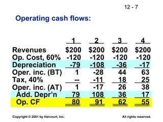
© 2001 by Harcourt, Inc. All rights reserved. Operating cash flows: 1 2 3 4 Revenues $200 $200 $200 $200 Op. Cost, 60% -120 -120 -120 -120 Depreciation -79 -108 -36 -17 Oper. inc. (BT) 1 -28 44 63 Tax, 40% -- -11 18 25 1 -17 26 38 Add. Depr’n 79 108 36 17 Op. CF 80 91 62 55 Oper. inc. (AT)
8.
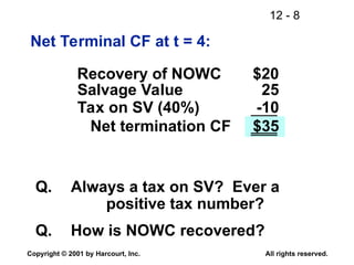
12 - 8 Copyright
© 2001 by Harcourt, Inc. All rights reserved. Net Terminal CF at t = 4: Salvage Value 25 Tax on SV (40%) -10 Recovery of NOWC $20 Net termination CF $35 Q. Always a tax on SV? Ever a positive tax number? Q. How is NOWC recovered?
9.
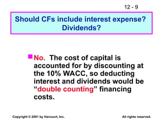
12 - 9 Copyright
© 2001 by Harcourt, Inc. All rights reserved. Should CFs include interest expense? Dividends? No. The cost of capital is accounted for by discounting at the 10% WACC, so deducting interest and dividends would be “double counting” financing costs.
10.
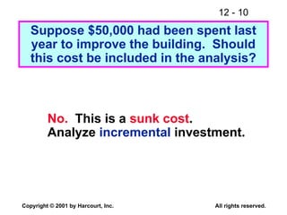
12 - 10 Copyright
© 2001 by Harcourt, Inc. All rights reserved. Suppose $50,000 had been spent last year to improve the building. Should this cost be included in the analysis? No. This is a sunk cost. Analyze incremental investment.
11.
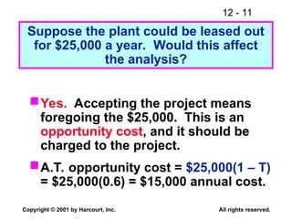
12 - 11 Copyright
© 2001 by Harcourt, Inc. All rights reserved. Suppose the plant could be leased out for $25,000 a year. Would this affect the analysis? Yes. Accepting the project means foregoing the $25,000. This is an opportunity cost, and it should be charged to the project. A.T. opportunity cost = $25,000(1 – T) = $25,000(0.6) = $15,000 annual cost.
12.
12 - 12 Copyright
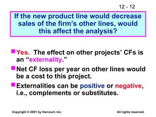
© 2001 by Harcourt, Inc. All rights reserved. If the new product line would decrease sales of the firm’s other lines, would this affect the analysis? Yes. The effect on other projects’ CFs is an “externality.” Net CF loss per year on other lines would be a cost to this project. Externalities can be positive or negative, i.e., complements or substitutes.
13.
12 - 13 Copyright
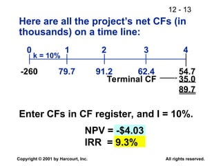
© 2001 by Harcourt, Inc. All rights reserved. Here are all the project’s net CFs (in thousands) on a time line: Enter CFs in CF register, and I = 10%. NPV = -$4.03 IRR = 9.3% k = 10% 0 79.7 1 91.2 2 62.4 3 54.7 4 -260 Terminal CF 35.0 89.7
14.
12 - 14 Copyright
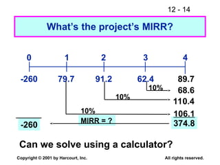
© 2001 by Harcourt, Inc. All rights reserved. MIRR = ? 10% What’s the project’s MIRR? Can we solve using a calculator? 0 79.7 1 91.2 2 62.4 3 89.7 4 -260 374.8 -260 68.6 110.4 10% 10% 106.1
15.
12 - 15 Copyright
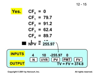
© 2001 by Harcourt, Inc. All rights reserved. 4 10 -255.97 0 TV = FV = 374.8 Yes. CF0 = 0 CF1 = 79.7 CF2 = 91.2 CF3 = 62.4 CF4 = 89.7 I = 10 NPV = 255.97 INPUTS OUTPUT N I/YR PV PMT FV
16.
12 - 16 Copyright
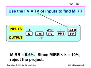
© 2001 by Harcourt, Inc. All rights reserved. Use the FV = TV of inputs to find MIRR 4 -260 0 374.8 9.6 MIRR = 9.6%. Since MIRR < k = 10%, reject the project. INPUTS OUTPUT N I/YR PV PMT FV
17.
12 - 17 Copyright
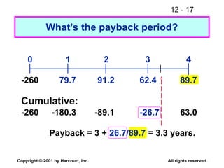
© 2001 by Harcourt, Inc. All rights reserved. What’s the payback period? 0 79.7 1 91.2 2 62.4 3 89.7 4 -260 Cumulative: -26.7 -260 -89.1 -180.3 63.0 Payback = 3 + 26.7/89.7 = 3.3 years.
18.
12 - 18 Copyright
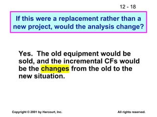
© 2001 by Harcourt, Inc. All rights reserved. If this were a replacement rather than a new project, would the analysis change? Yes. The old equipment would be sold, and the incremental CFs would be the changes from the old to the new situation.
19.
12 - 19 Copyright
© 2001 by Harcourt, Inc. All rights reserved. The relevant depreciation would be the change with the new equipment. Also, if the firm sold the old machine now, it would not receive the SV at the end of the machine’s life. This is an opportunity cost for the replacement project.
20.
12 - 20 Copyright
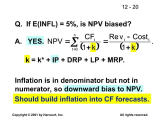
© 2001 by Harcourt, Inc. All rights reserved. . k 1 Cost v Re k 1 CF NPV t t t t t n 0 t Q. If E(INFL) = 5%, is NPV biased? A. YES. k = k* + IP + DRP + LP + MRP. Inflation is in denominator but not in numerator, so downward bias to NPV. Should build inflation into CF forecasts.
21.
12 - 21 Copyright
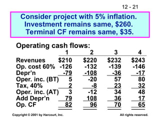
© 2001 by Harcourt, Inc. All rights reserved. Consider project with 5% inflation. Investment remains same, $260. Terminal CF remains same, $35. Operating cash flows: 1 2 3 4 Revenues $210 $220 $232 $243 Op. cost 60% -126 -132 -139 -146 Depr’n -79 -108 -36 -17 Oper. inc. (BT) 5 -20 57 80 Tax, 40% 2 -8 23 32 Oper. inc. (AT) 3 -12 34 48 Add Depr’n 79 108 36 17 Op. CF 82 96 70 65
22.
12 - 22 Copyright
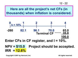
© 2001 by Harcourt, Inc. All rights reserved. Here are all the project’s net CFs (in thousands) when inflation is considered. Enter CFs in CF register, and I = 10%. NPV = $15.0 IRR = 12.6% k = 10% 0 82.1 1 96.1 2 70.0 3 65.0 4 -260 Terminal CF 35.0 100.0 Project should be accepted.
23.
12 - 23 Copyright
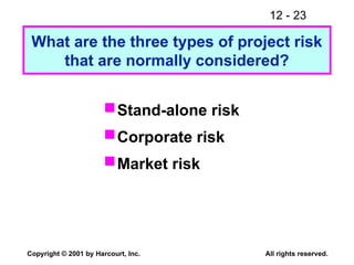
© 2001 by Harcourt, Inc. All rights reserved. What are the three types of project risk that are normally considered? Stand-alone risk Corporate risk Market risk
24.
12 - 24 Copyright
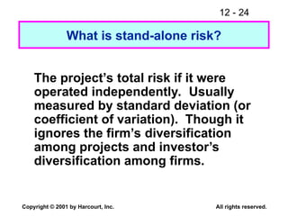
© 2001 by Harcourt, Inc. All rights reserved. What is stand-alone risk? The project’s total risk if it were operated independently. Usually measured by standard deviation (or coefficient of variation). Though it ignores the firm’s diversification among projects and investor’s diversification among firms.
25.
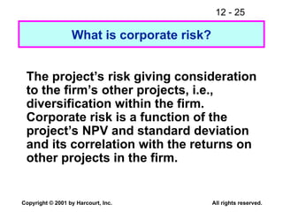
12 - 25 Copyright
© 2001 by Harcourt, Inc. All rights reserved. What is corporate risk? The project’s risk giving consideration to the firm’s other projects, i.e., diversification within the firm. Corporate risk is a function of the project’s NPV and standard deviation and its correlation with the returns on other projects in the firm.
26.
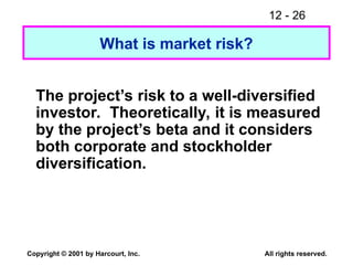
12 - 26 Copyright
© 2001 by Harcourt, Inc. All rights reserved. What is market risk? The project’s risk to a well-diversified investor. Theoretically, it is measured by the project’s beta and it considers both corporate and stockholder diversification.
27.
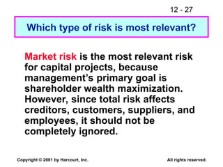
12 - 27 Copyright
© 2001 by Harcourt, Inc. All rights reserved. Which type of risk is most relevant? Market risk is the most relevant risk for capital projects, because management’s primary goal is shareholder wealth maximization. However, since total risk affects creditors, customers, suppliers, and employees, it should not be completely ignored.
28.
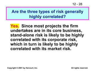
12 - 28 Copyright
© 2001 by Harcourt, Inc. All rights reserved. Are the three types of risk generally highly correlated? Yes. Since most projects the firm undertakes are in its core business, stand-alone risk is likely to be highly correlated with its corporate risk, which in turn is likely to be highly correlated with its market risk.
29.
12 - 29 Copyright
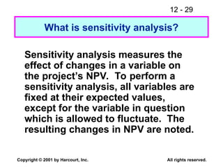
© 2001 by Harcourt, Inc. All rights reserved. What is sensitivity analysis? Sensitivity analysis measures the effect of changes in a variable on the project’s NPV. To perform a sensitivity analysis, all variables are fixed at their expected values, except for the variable in question which is allowed to fluctuate. The resulting changes in NPV are noted.
30.
12 - 30 Copyright
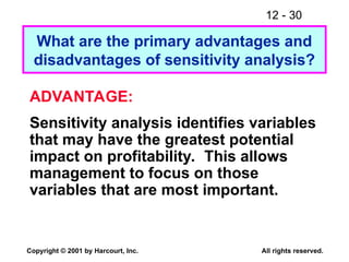
© 2001 by Harcourt, Inc. All rights reserved. What are the primary advantages and disadvantages of sensitivity analysis? ADVANTAGE: Sensitivity analysis identifies variables that may have the greatest potential impact on profitability. This allows management to focus on those variables that are most important.
31.
12 - 31 Copyright
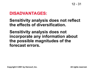
© 2001 by Harcourt, Inc. All rights reserved. DISADVANTAGES: Sensitivity analysis does not reflect the effects of diversification. Sensitivity analysis does not incorporate any information about the possible magnitudes of the forecast errors.
32.
12 - 32 Copyright
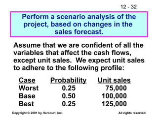
© 2001 by Harcourt, Inc. All rights reserved. Best 0.25 125,000 Perform a scenario analysis of the project, based on changes in the sales forecast. Assume that we are confident of all the variables that affect the cash flows, except unit sales. We expect unit sales to adhere to the following profile: Case Probability Unit sales Base 0.50 100,000 Worst 0.25 75,000
33.
12 - 33 Copyright
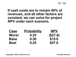
© 2001 by Harcourt, Inc. All rights reserved. If cash costs are to remain 60% of revenues, and all other factors are constant, we can solve for project NPV under each scenario. Best 0.25 $57.8 Case Probability NPV Base 0.50 $15.0 Worst 0.25 ($27.8)
34.
12 - 34 Copyright
© 2001 by Harcourt, Inc. All rights reserved. E(NPV)=.25(-$27.8)+.5($15.0)+.25($57.8) E(NPV)= $15.0. Use these scenarios, with their given probabilities, to find the project’s expected NPV, NPV, and CVNPV. NPV = [.25(-$27.8-$15.0)2 + .5($15.0-$15.0)2 + .25($57.8-$15.0)2 ]1/2 NPV = $30.3. CVNPV = $30.3 /$15.0 = 2.0.
35.
12 - 35 Copyright
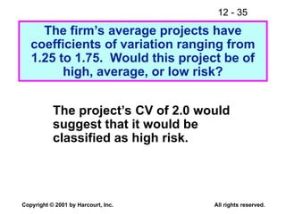
© 2001 by Harcourt, Inc. All rights reserved. The firm’s average projects have coefficients of variation ranging from 1.25 to 1.75. Would this project be of high, average, or low risk? The project’s CV of 2.0 would suggest that it would be classified as high risk.
36.
12 - 36 Copyright
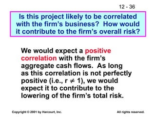
© 2001 by Harcourt, Inc. All rights reserved. Is this project likely to be correlated with the firm’s business? How would it contribute to the firm’s overall risk? We would expect a positive correlation with the firm’s aggregate cash flows. As long as this correlation is not perfectly positive (i.e., r 1), we would expect it to contribute to the lowering of the firm’s total risk.
37.
12 - 37 Copyright
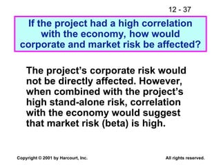
© 2001 by Harcourt, Inc. All rights reserved. The project’s corporate risk would not be directly affected. However, when combined with the project’s high stand-alone risk, correlation with the economy would suggest that market risk (beta) is high. If the project had a high correlation with the economy, how would corporate and market risk be affected?
38.
12 - 38 Copyright
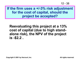
© 2001 by Harcourt, Inc. All rights reserved. Reevaluating this project at a 13% cost of capital (due to high stand- alone risk), the NPV of the project is -$2.2 . If the firm uses a +/-3% risk adjustment for the cost of capital, should the project be accepted?
39.
12 - 39 Copyright
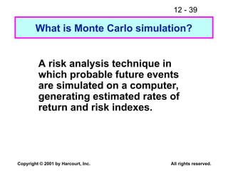
© 2001 by Harcourt, Inc. All rights reserved. A risk analysis technique in which probable future events are simulated on a computer, generating estimated rates of return and risk indexes. What is Monte Carlo simulation?
Download


![12 - 34
Copyright © 2001 by Harcourt, Inc. All rights reserved.
E(NPV)=.25(-$27.8)+.5($15.0)+.25($57.8)
E(NPV)= $15.0.
Use these scenarios, with their given
probabilities, to find the project’s
expected NPV, NPV, and CVNPV.
NPV = [.25(-$27.8-$15.0)2
+ .5($15.0-$15.0)2
+ .25($57.8-$15.0)2
]1/2
NPV = $30.3.
CVNPV = $30.3 /$15.0 = 2.0.](https://image.slidesharecdn.com/ffm912-cash-flow-estimation-and-risk-analysis-251025202856-cc48c2d3/85/ffm912-cash-flow-estimation-and-risk-analysis-ppt-34-320.jpg)


![1. Payback Period and Net Present Value[LO1, 2] If a project with .docx](https://cdn.slidesharecdn.com/ss_thumbnails/1-221101035238-1d86b81e-thumbnail.jpg?width=640&height=640&fit=bounds)


