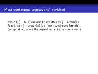
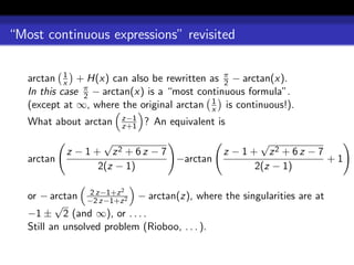
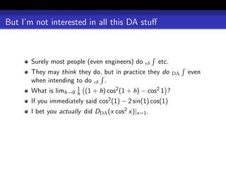
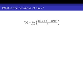
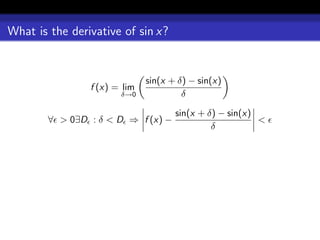
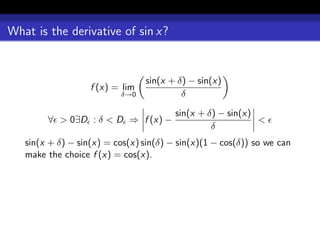
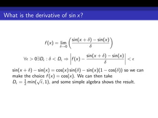
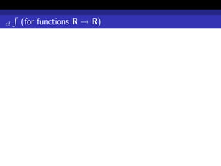
The document discusses fundamental concepts in calculus, particularly focusing on the derivatives and integrals of trigonometric functions like sin(x) and cos(x), exploring the underlying limits and algebraic principles. It raises questions about the teaching and understanding of these concepts, such as the effectiveness of algebra in deriving these results. The text further delves into the fundamental theorem of calculus and the significance of differentiation and its applications in different mathematical contexts.


![π/2
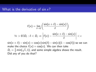
What is the integral: 0 cos x?
I = lim S ∆ [cos(x)] = lim S ∆ [cos(x)]
|∆|→0 |∆|→0
(∆ ranges over all dissections of [0, π/2])](https://image.slidesharecdn.com/caims-124547011297-phpapp02/85/Caims-2009-11-320.jpg)
![π/2
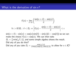
What is the integral: 0 cos x?
I = lim S ∆ [cos(x)] = lim S ∆ [cos(x)]
|∆|→0 |∆|→0
(∆ ranges over all dissections of [0, π/2])
Does anyone actually do this?](https://image.slidesharecdn.com/caims-124547011297-phpapp02/85/Caims-2009-12-320.jpg)
![π/2
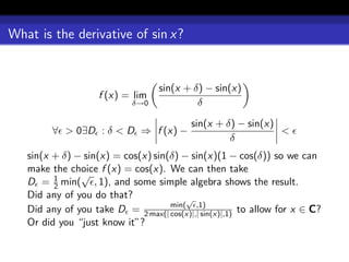
What is the integral: 0 cos x?
I = lim S ∆ [cos(x)] = lim S ∆ [cos(x)]
|∆|→0 |∆|→0
(∆ ranges over all dissections of [0, π/2])
Does anyone actually do this?
Can anyone actually do this?](https://image.slidesharecdn.com/caims-124547011297-phpapp02/85/Caims-2009-13-320.jpg)
![π/2
What is the integral: 0 cos x?
I = lim S ∆ [cos(x)] = lim S ∆ [cos(x)]
|∆|→0 |∆|→0
(∆ ranges over all dissections of [0, π/2])
Does anyone actually do this?
Can anyone actually do this?
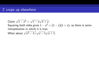
Or do we say “well, we have proved that sin = cos, so cos = sin,
and therefore the answer is sin π − sin 0 = 1?
2](https://image.slidesharecdn.com/caims-124547011297-phpapp02/85/Caims-2009-14-320.jpg)
![π/2
What is the integral: 0 cos x?
I = lim S ∆ [cos(x)] = lim S ∆ [cos(x)]
|∆|→0 |∆|→0
(∆ ranges over all dissections of [0, π/2])
Does anyone actually do this?
Can anyone actually do this?
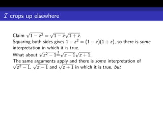
Or do we say “well, we have proved that sin = cos, so cos = sin,
and therefore the answer is sin π − sin 0 = 1?
2
We might say “therefore, by the Fundamental Theorem of
Calculus, . . . ”](https://image.slidesharecdn.com/caims-124547011297-phpapp02/85/Caims-2009-15-320.jpg)
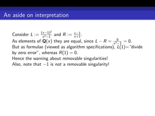
![What is the Fundamental Theorem of Calculus?
Indeed, what is calculus?
. . . the deism of Liebniz over the dotage of Newton . . .
[Babbage, chapter 4]](https://image.slidesharecdn.com/caims-124547011297-phpapp02/85/Caims-2009-18-320.jpg)
![What is the Fundamental Theorem of Calculus?
Indeed, what is calculus?
. . . the deism of Liebniz over the dotage of Newton . . .
[Babbage, chapter 4]
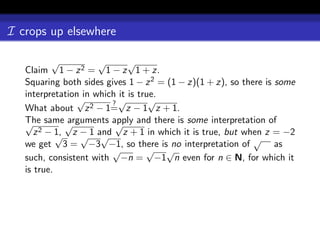
I claim that calculus is actually the interesting fusion of two,
different subjects.](https://image.slidesharecdn.com/caims-124547011297-phpapp02/85/Caims-2009-19-320.jpg)
![What is the Fundamental Theorem of Calculus?
Indeed, what is calculus?
. . . the deism of Liebniz over the dotage of Newton . . .
[Babbage, chapter 4]
I claim that calculus is actually the interesting fusion of two,
different subjects.
What you learned in calculus, which I shall write as D δ : the
“differentiation of –δ analysis”. Also d d x , and its inverse
δ
δ .](https://image.slidesharecdn.com/caims-124547011297-phpapp02/85/Caims-2009-20-320.jpg)
![What is the Fundamental Theorem of Calculus?
Indeed, what is calculus?
. . . the deism of Liebniz over the dotage of Newton . . .
[Babbage, chapter 4]
I claim that calculus is actually the interesting fusion of two,
different subjects.
What you learned in calculus, which I shall write as D δ : the
“differentiation of –δ analysis”. Also d d x , and its inverse
δ
δ .
What is taught in differential algebra, which I shall write as
d
DDA : the “differentiation of differential algebra”. Also dDA x ,
and its inverse DA .](https://image.slidesharecdn.com/caims-124547011297-phpapp02/85/Caims-2009-21-320.jpg)
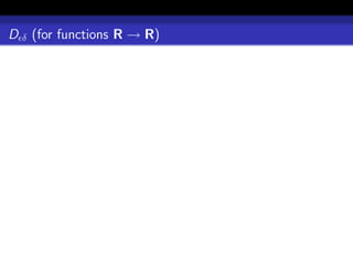


![How are the two subjects related?
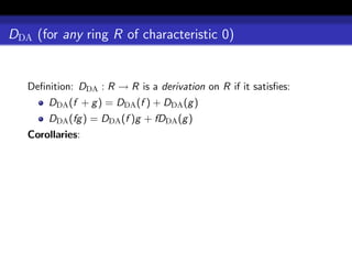
If we define DDA (x) = 1, then DDA is defined on Z[x], and
extends to Q(x) and indeed Q(x).](https://image.slidesharecdn.com/caims-124547011297-phpapp02/85/Caims-2009-44-320.jpg)
![How are the two subjects related?
If we define DDA (x) = 1, then DDA is defined on Z[x], and
extends to Q(x) and indeed Q(x).
If we interpret (denoted I) Q(x) as functions R → R, then DDA
can be interpreted as D δ , i.e.
I(DDA (f )) = D δ (I(f ))](https://image.slidesharecdn.com/caims-124547011297-phpapp02/85/Caims-2009-45-320.jpg)
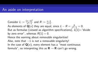
![How are the two subjects related?
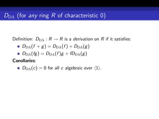
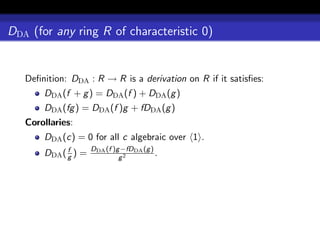
If we define DDA (x) = 1, then DDA is defined on Z[x], and
extends to Q(x) and indeed Q(x).
If we interpret (denoted I) Q(x) as functions R → R, then DDA
can be interpreted as D δ , i.e.
I(DDA (f )) = D δ (I(f ))
(at least up to removable singularities).](https://image.slidesharecdn.com/caims-124547011297-phpapp02/85/Caims-2009-46-320.jpg)
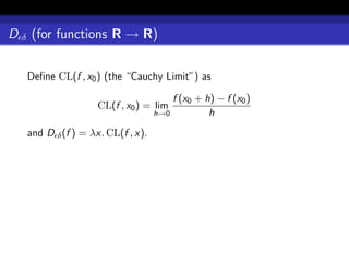
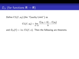
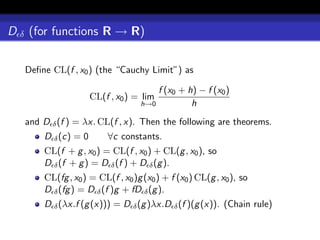
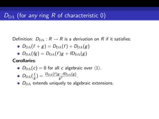
![δ (for functions R → R)
What is naturally defined is integration over an interval I . We let
D stand for sub-divisions d1 = a < d2 < · · · < dn = b of I = [a, b],
and |D| for the largest distance between neighbouring points in D,
i.e. maxi (di+1 − di ).](https://image.slidesharecdn.com/caims-124547011297-phpapp02/85/Caims-2009-56-320.jpg)
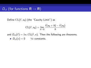
![δ (for functions R → R)
What is naturally defined is integration over an interval I . We let
D stand for sub-divisions d1 = a < d2 < · · · < dn = b of I = [a, b],
and |D| for the largest distance between neighbouring points in D,
i.e. maxi (di+1 − di ). Let
SD = i (di+1 − di ) maxdi+1 ≥x≥di f (x);](https://image.slidesharecdn.com/caims-124547011297-phpapp02/85/Caims-2009-57-320.jpg)
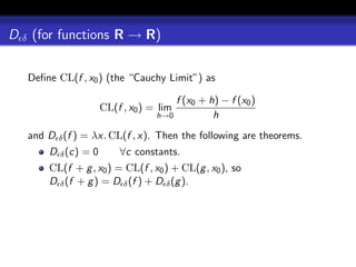
![δ (for functions R → R)
What is naturally defined is integration over an interval I . We let
D stand for sub-divisions d1 = a < d2 < · · · < dn = b of I = [a, b],
and |D| for the largest distance between neighbouring points in D,
i.e. maxi (di+1 − di ). Let
SD = i (di+1 − di ) maxdi+1 ≥x≥di f (x);
SD = i (di+1 − di ) mindi+1 ≥x≥di f (x);](https://image.slidesharecdn.com/caims-124547011297-phpapp02/85/Caims-2009-58-320.jpg)
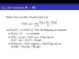
![δ (for functions R → R)
What is naturally defined is integration over an interval I . We let
D stand for sub-divisions d1 = a < d2 < · · · < dn = b of I = [a, b],
and |D| for the largest distance between neighbouring points in D,
i.e. maxi (di+1 − di ). Let
SD = i (di+1 − di ) maxdi+1 ≥x≥di f (x);
SD = i (di+1 − di ) mindi+1 ≥x≥di f (x);
Then δ I f = lim inf |D|→0 SD = lim sup|D|→0 SD if both exist and
are equal.](https://image.slidesharecdn.com/caims-124547011297-phpapp02/85/Caims-2009-59-320.jpg)
![Consequences: Fundamental Theorem of Calculus (FTC δ )
b δ [a,b] f a≤b
Define δ a f =
− δ [b,a] f a>b](https://image.slidesharecdn.com/caims-124547011297-phpapp02/85/Caims-2009-60-320.jpg)
![Consequences: Fundamental Theorem of Calculus (FTC δ )
b δ [a,b] f a≤b
Define δ a f =
− δ [b,a] f a > b
(If we’re not careful, we wind up saying “[2,1] is the same set as
[1,2] except that if you integrate over it you have to add a −
sign”. What we really have here is the beginnings of contour
integration.](https://image.slidesharecdn.com/caims-124547011297-phpapp02/85/Caims-2009-61-320.jpg)
![Consequences: Fundamental Theorem of Calculus (FTC δ )
b δ [a,b] f a≤b
Define δ a f =
− δ [b,a] f a > b
(If we’re not careful, we wind up saying “[2,1] is the same set as
[1,2] except that if you integrate over it you have to add a −
sign”. What we really have here is the beginnings of contour
integration. Apostol theorem 1.20 states that if g (x) ≤ f (x) for
every x in [a, b], then
b b
g (x)dx ≤ f (x)dx,
a a
and here a < b is implicit.)](https://image.slidesharecdn.com/caims-124547011297-phpapp02/85/Caims-2009-62-320.jpg)
![Consequences: Fundamental Theorem of Calculus (FTC δ )
b δ [a,b] f a≤b
Define δ a f =
− δ [b,a] f a > b
(If we’re not careful, we wind up saying “[2,1] is the same set as
[1,2] except that if you integrate over it you have to add a −
sign”. What we really have here is the beginnings of contour
integration. Apostol theorem 1.20 states that if g (x) ≤ f (x) for
every x in [a, b], then
b b
g (x)dx ≤ f (x)dx,
a a
and here a < b is implicit.)
FTC δ : δ [a,b] D δ f = f (b) − f (a).](https://image.slidesharecdn.com/caims-124547011297-phpapp02/85/Caims-2009-63-320.jpg)
![Consequences: Fundamental Theorem of Calculus (FTC δ )
b δ [a,b] f a≤b
Define δ a f =
− δ [b,a] f a > b
(If we’re not careful, we wind up saying “[2,1] is the same set as
[1,2] except that if you integrate over it you have to add a −
sign”. What we really have here is the beginnings of contour
integration. Apostol theorem 1.20 states that if g (x) ≤ f (x) for
every x in [a, b], then
b b
g (x)dx ≤ f (x)dx,
a a
and here a < b is implicit.)
FTC δ : δ [a,b] D δ f = f (b) − f (a).
x
Or: D δ (λx. δ a f ) = f (if the δ exists).](https://image.slidesharecdn.com/caims-124547011297-phpapp02/85/Caims-2009-64-320.jpg)
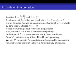
![Consequences: Fundamental Theorem of Calculus (FTC δ )
b δ [a,b] f a≤b
Define δ a f =
− δ [b,a] f a > b
(If we’re not careful, we wind up saying “[2,1] is the same set as
[1,2] except that if you integrate over it you have to add a −
sign”. What we really have here is the beginnings of contour
integration. Apostol theorem 1.20 states that if g (x) ≤ f (x) for
every x in [a, b], then
b b
g (x)dx ≤ f (x)dx,
a a
and here a < b is implicit.)
FTC δ : δ [a,b] D δ f = f (b) − f (a).
x
Or: D δ (λx. δ a f ) = f (if the δ exists).
(Of course, this is normally stated without the λ.)](https://image.slidesharecdn.com/caims-124547011297-phpapp02/85/Caims-2009-65-320.jpg)
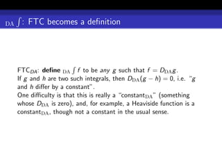


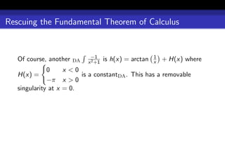
![Will the real FTC please stand up?
FTC (as it should be taught).
If g = DA f , and I(g ) is continuous on [a, b], then
b
δ I(f ) = I(g )(b) − I(g )(a).
a](https://image.slidesharecdn.com/caims-124547011297-phpapp02/85/Caims-2009-72-320.jpg)
![Will the real FTC please stand up?
FTC (as it should be taught).
If g = DA f , and I(g ) is continuous on [a, b], then
b
δ I(f ) = I(g )(b) − I(g )(a).
a
1
Note the caveat on continuity: g : x → arctan x is discontinuous
at x = 0 (limx→0− arctan x = −π whereas
1
2
limx→0+ arctan x = π ),
1
2](https://image.slidesharecdn.com/caims-124547011297-phpapp02/85/Caims-2009-73-320.jpg)
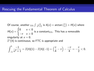
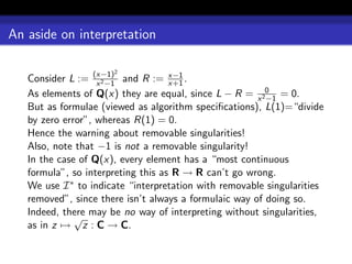
![Will the real FTC please stand up?
FTC (as it should be taught).
If g = DA f , and I(g ) is continuous on [a, b], then
b
δ I(f ) = I(g )(b) − I(g )(a).
a
1
Note the caveat on continuity: g : x → arctan x is discontinuous
1 −π
at x = 0 (limx→0− arctan x = 2 whereas
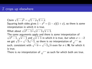
limx→0+ arctan x = π ), which accounts for the invalidity of
1
2
deducing that the integral of a negative function is positive —
1
−1 π −π π
= I(g )(1) − I(g )(−1) = − = > 0.
−1 x2+1 4 4 2](https://image.slidesharecdn.com/caims-124547011297-phpapp02/85/Caims-2009-74-320.jpg)