Download as PDF, PPTX

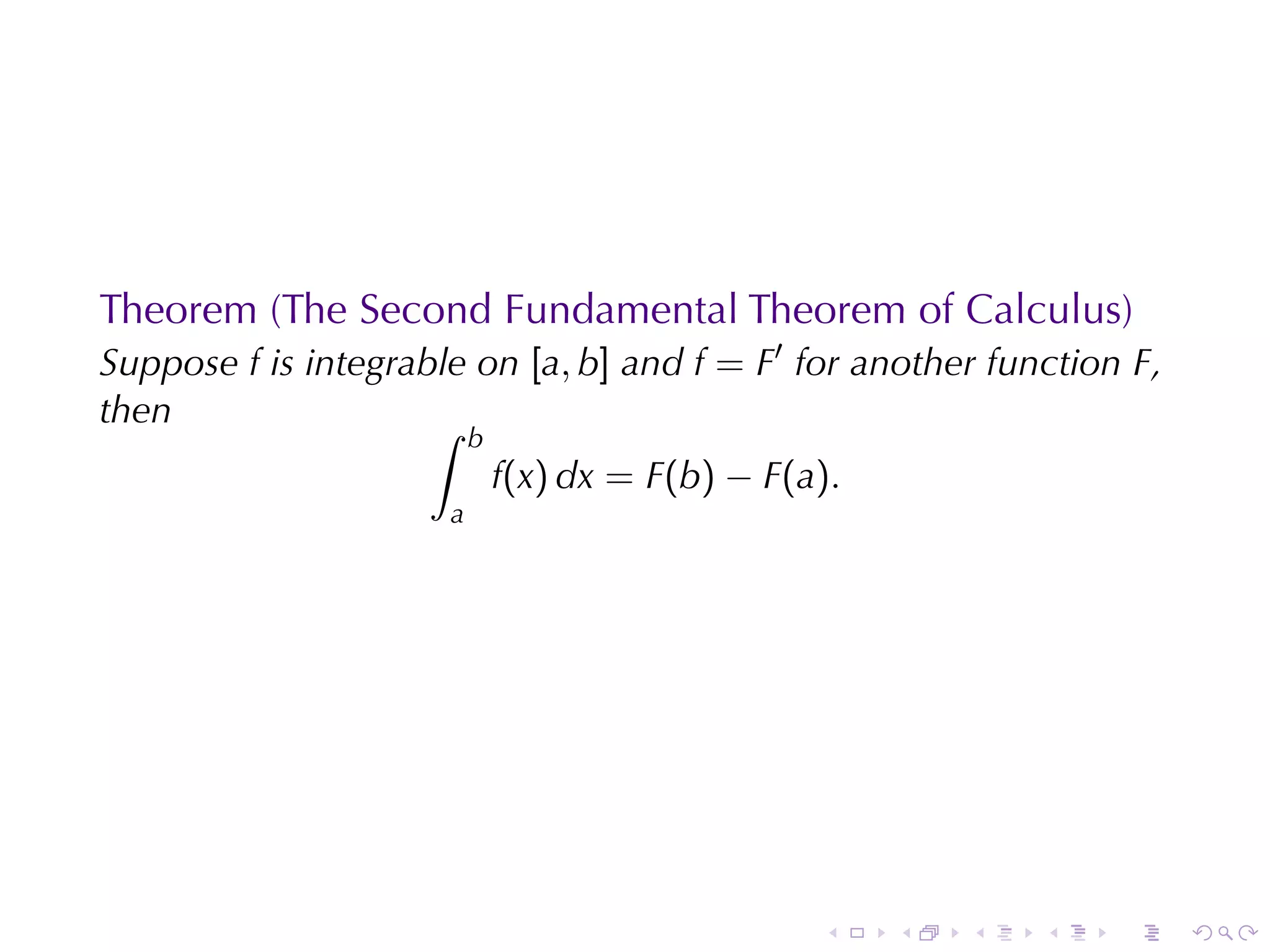
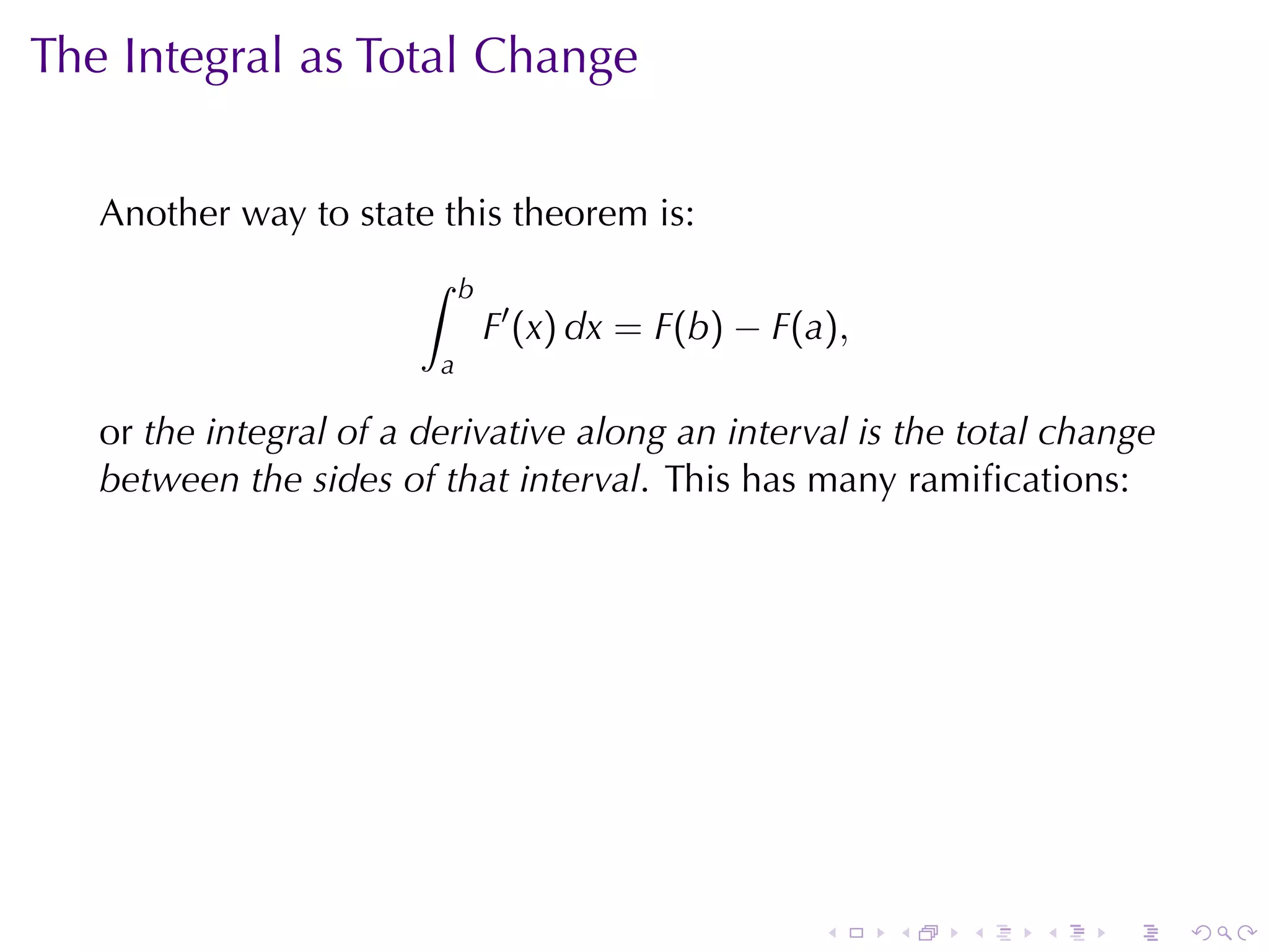
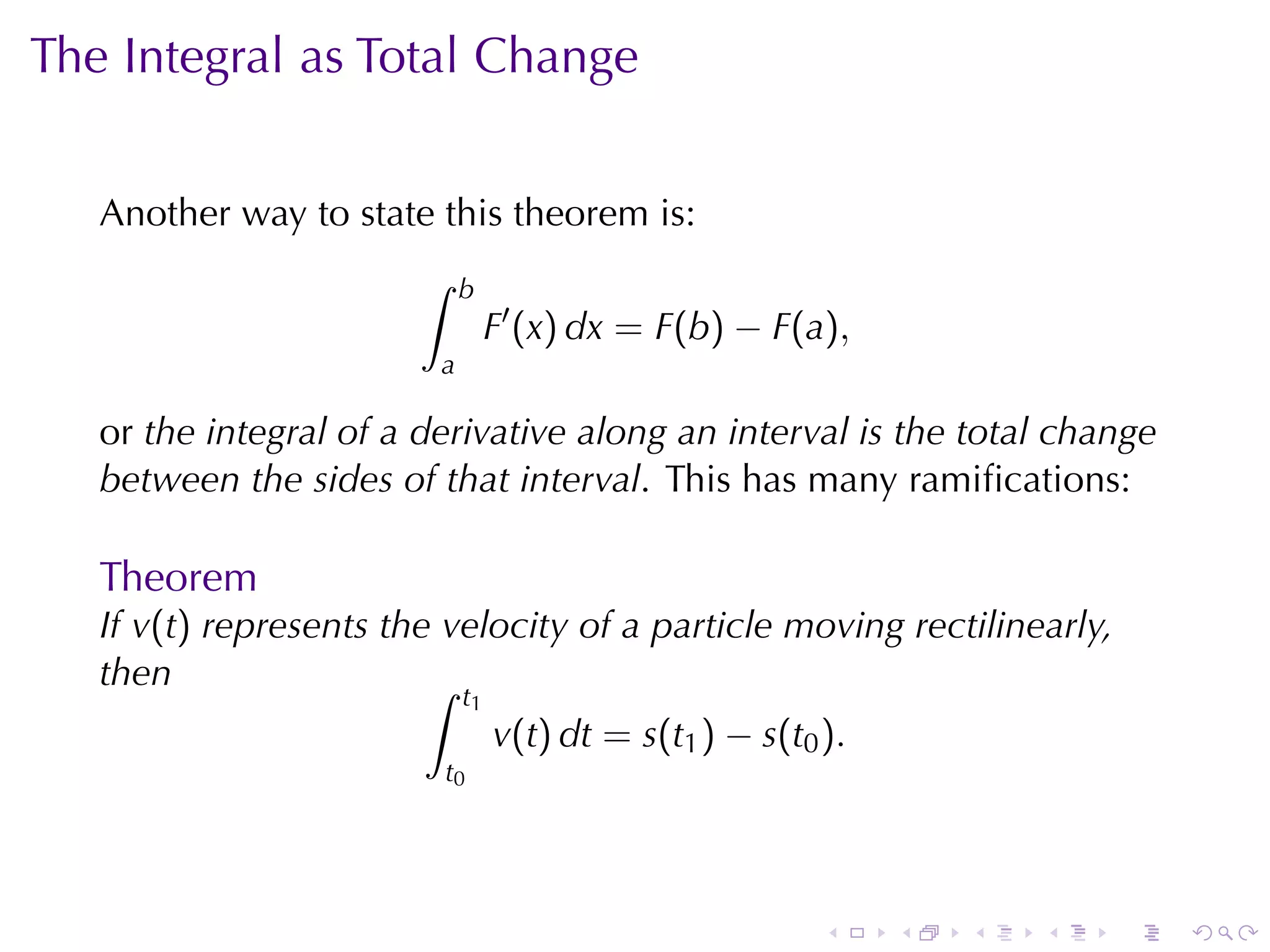
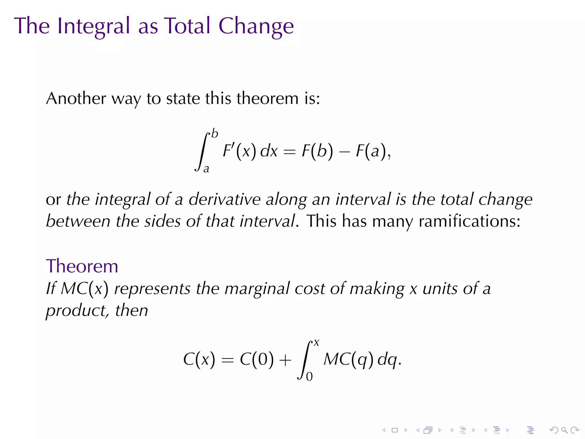
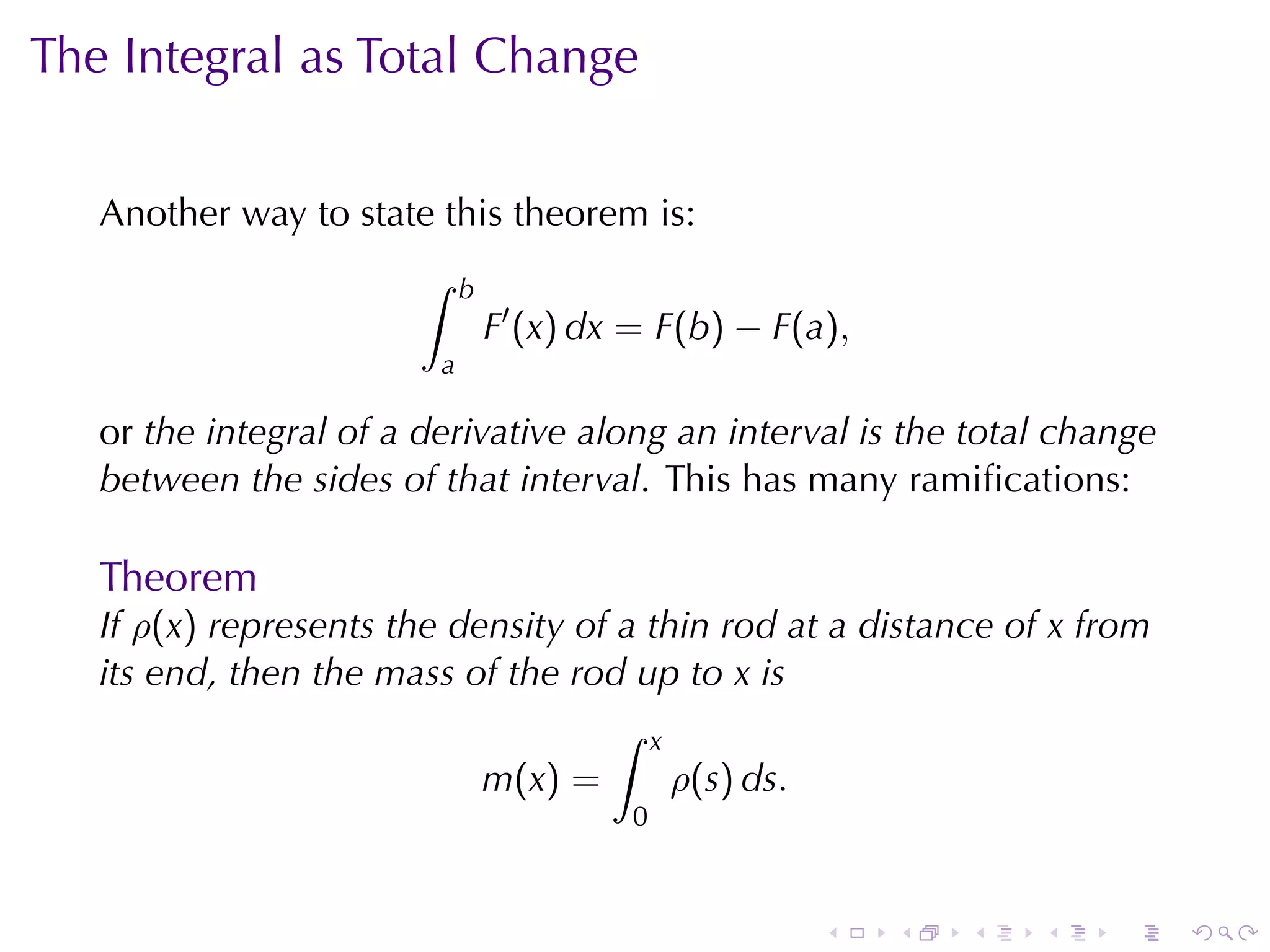
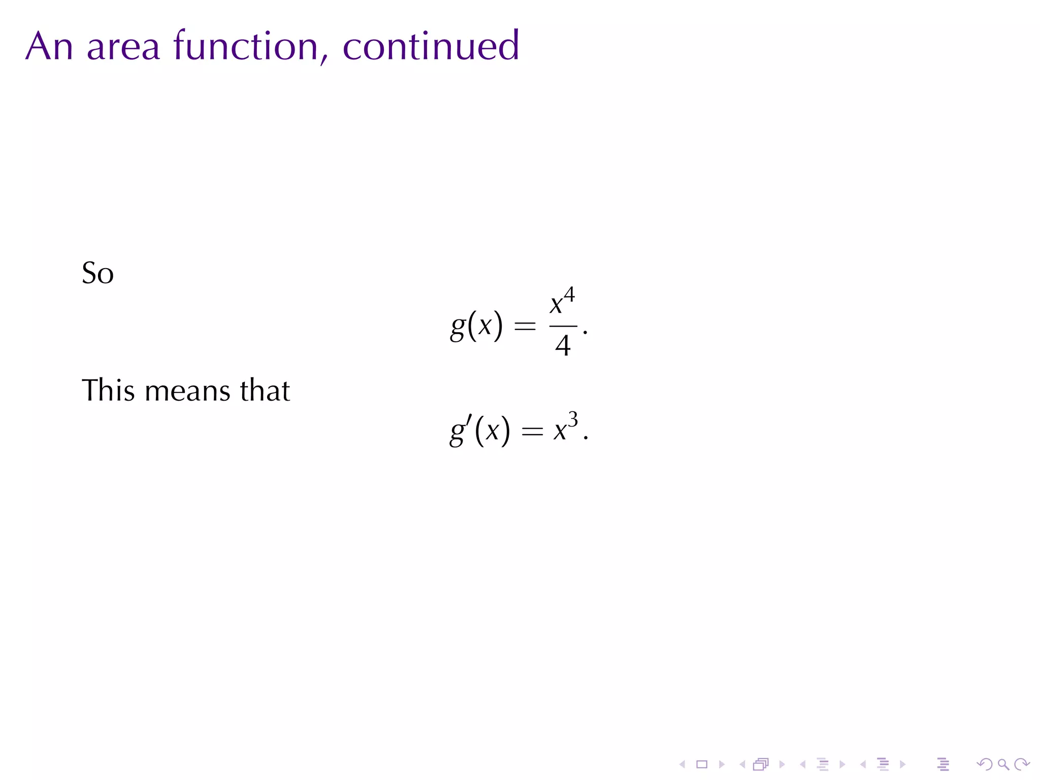
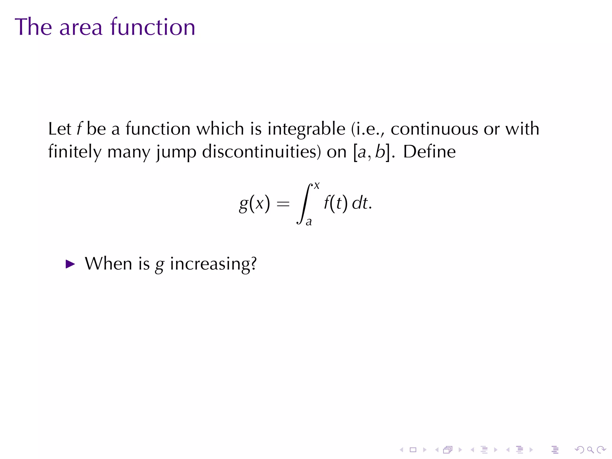
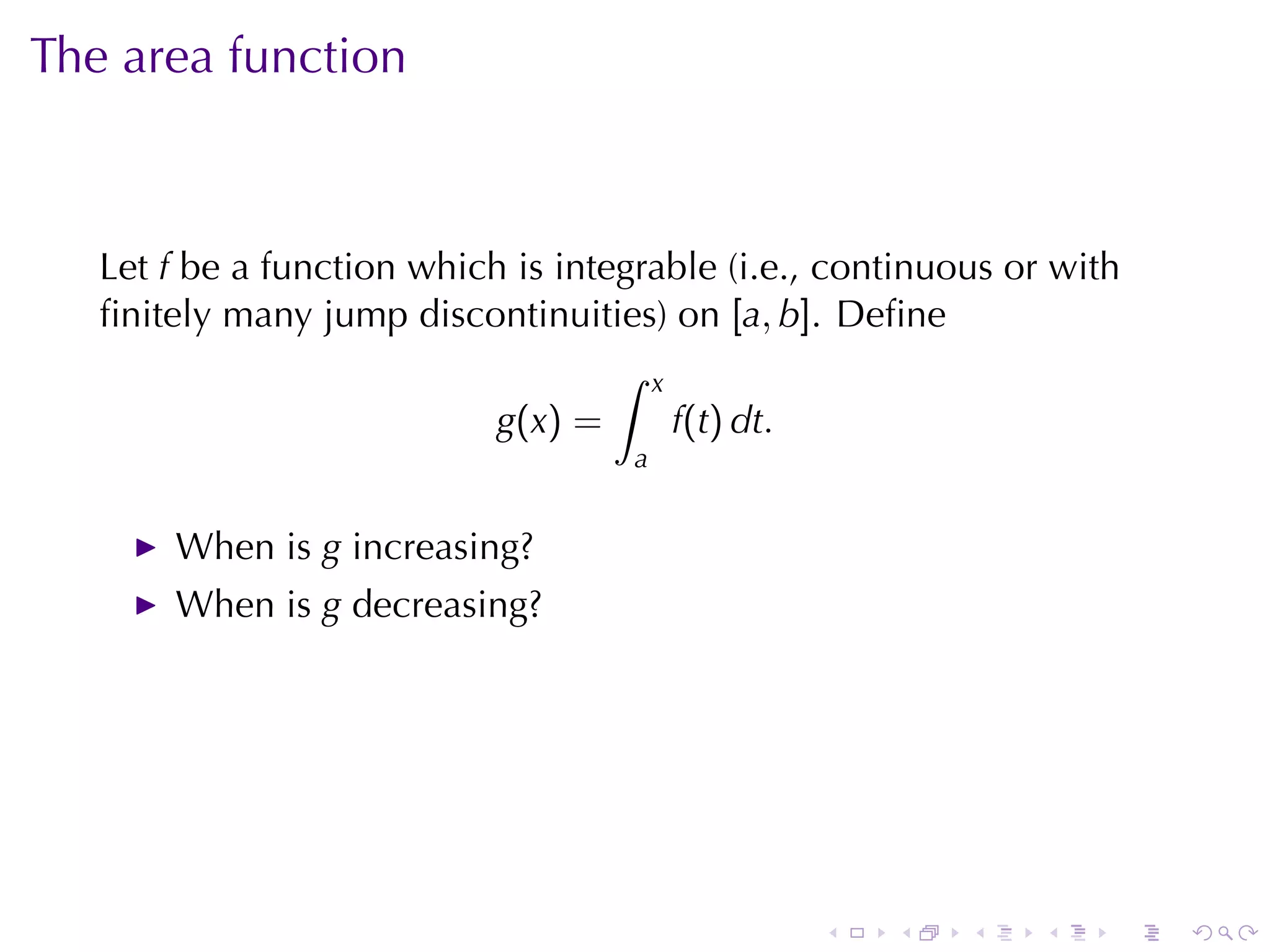
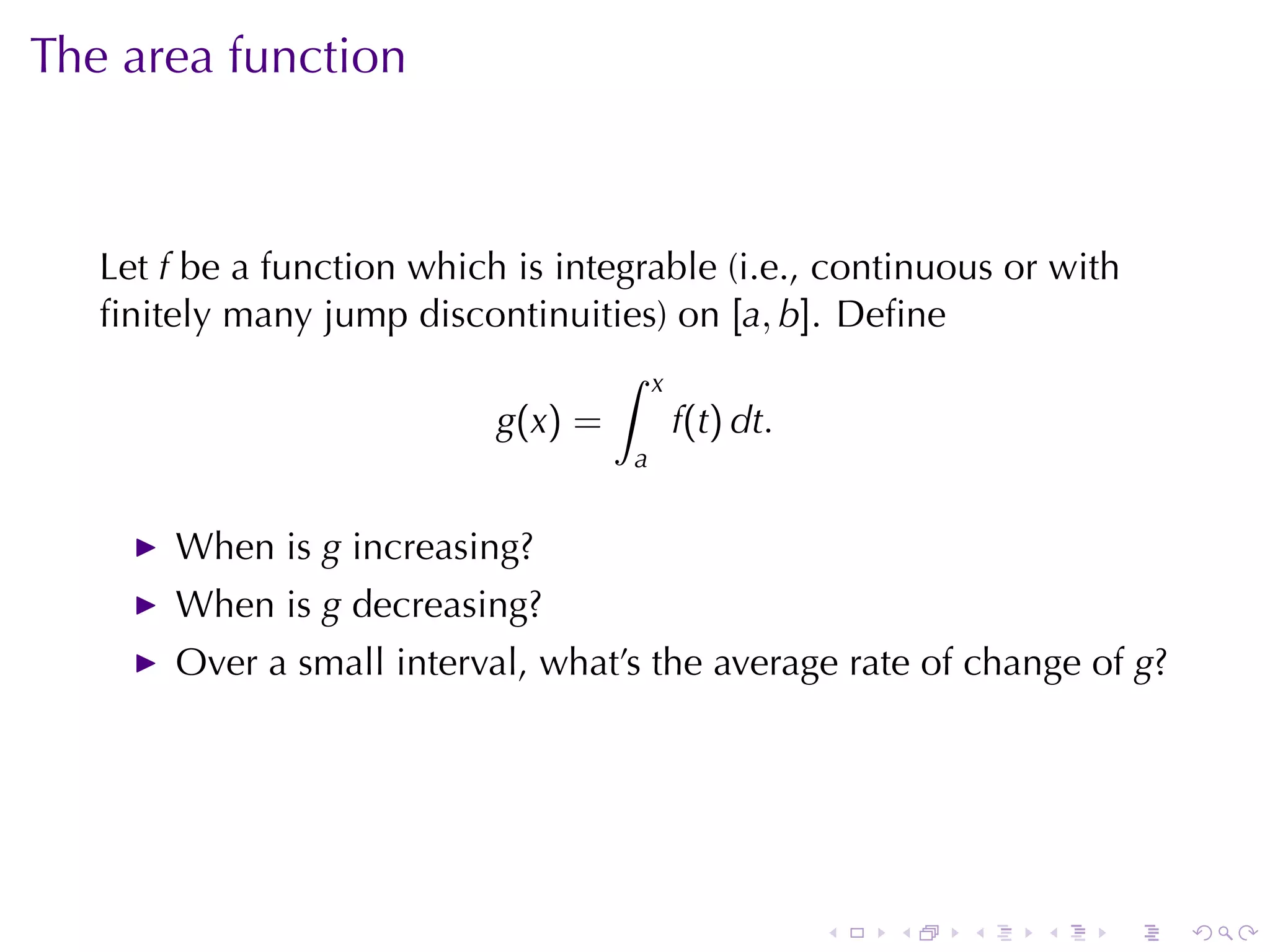
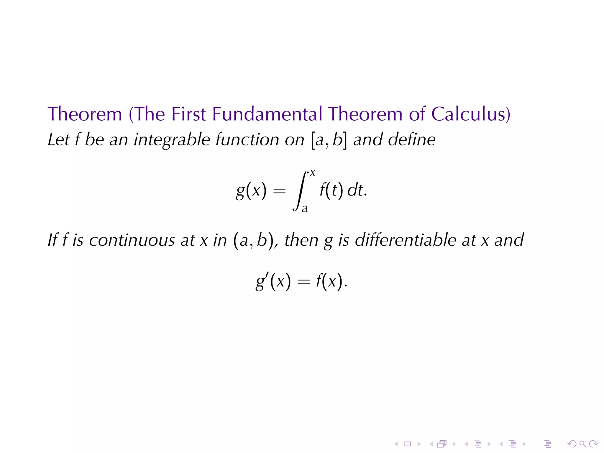
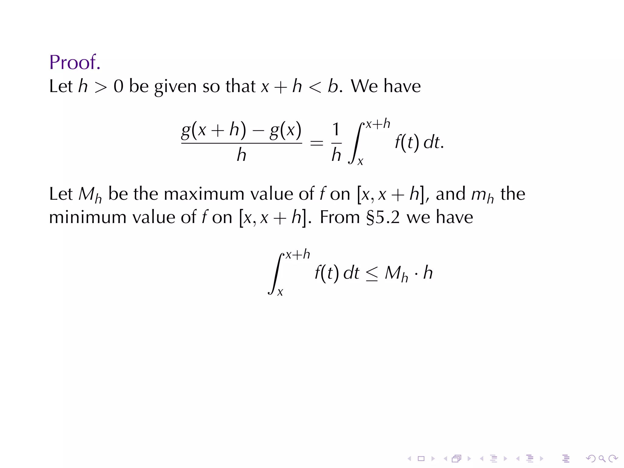
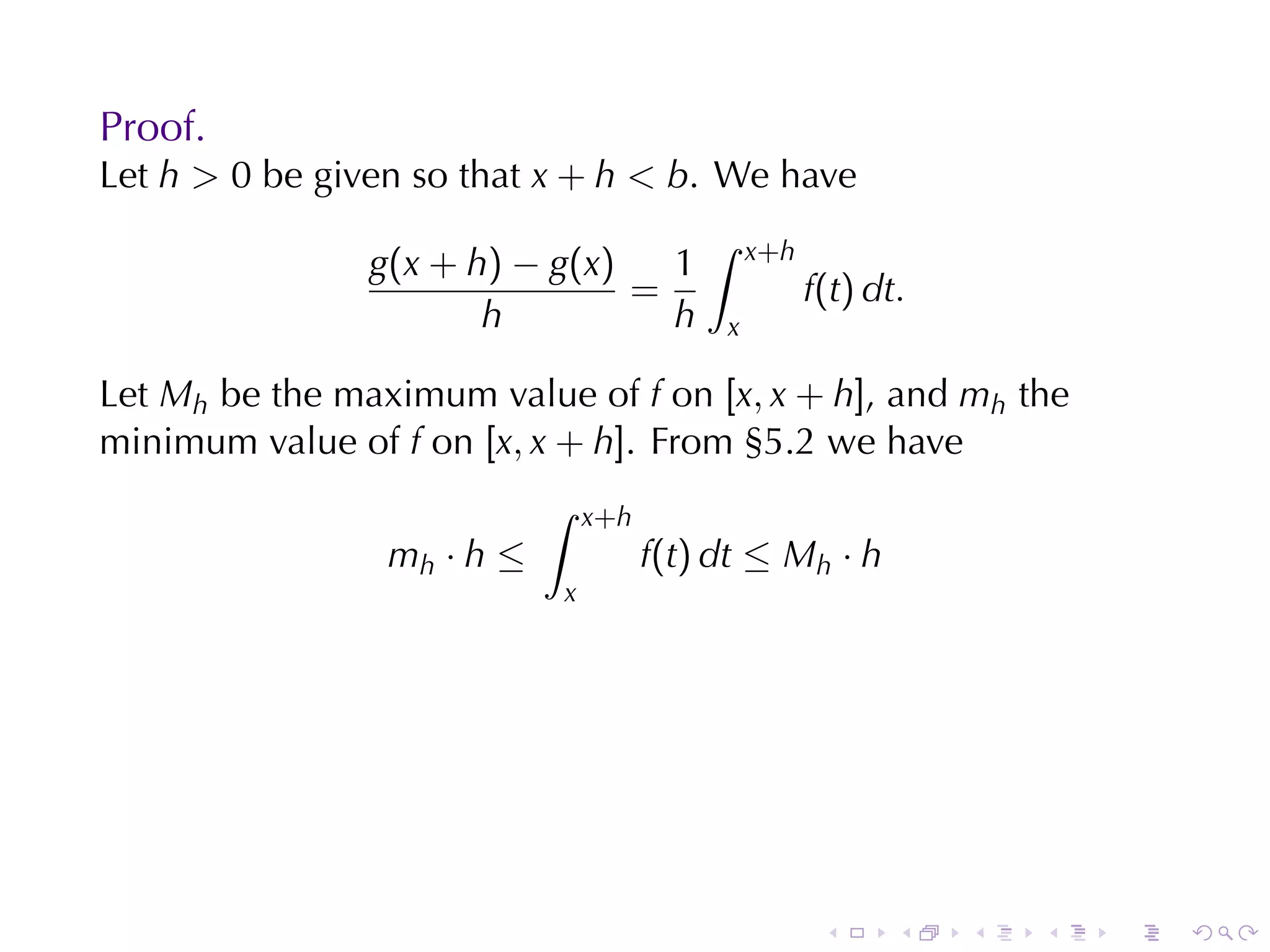
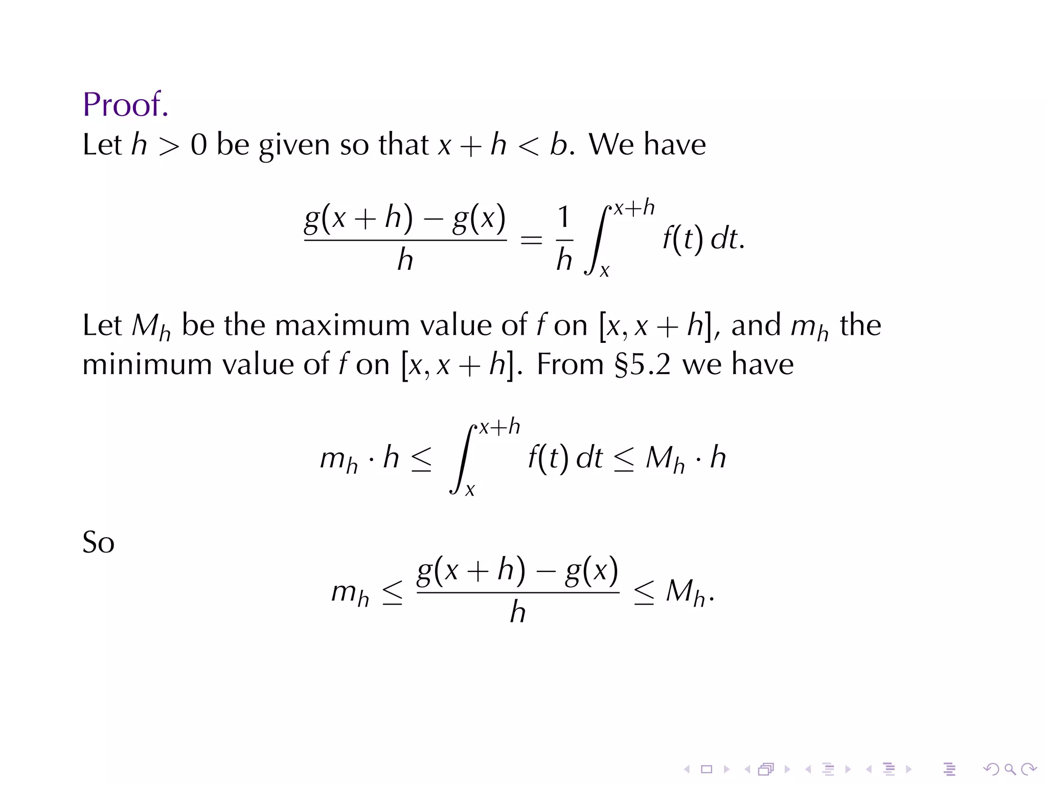
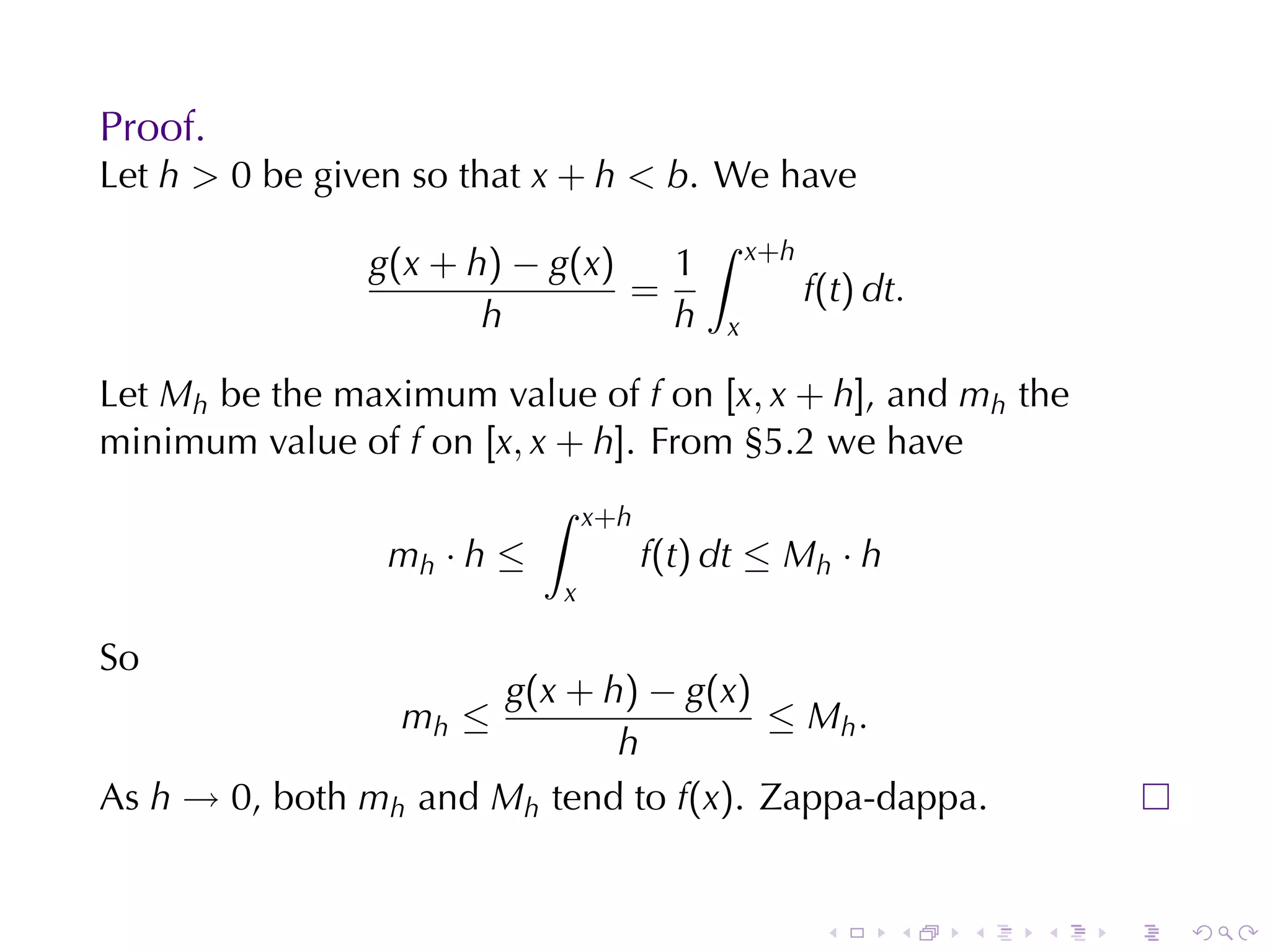


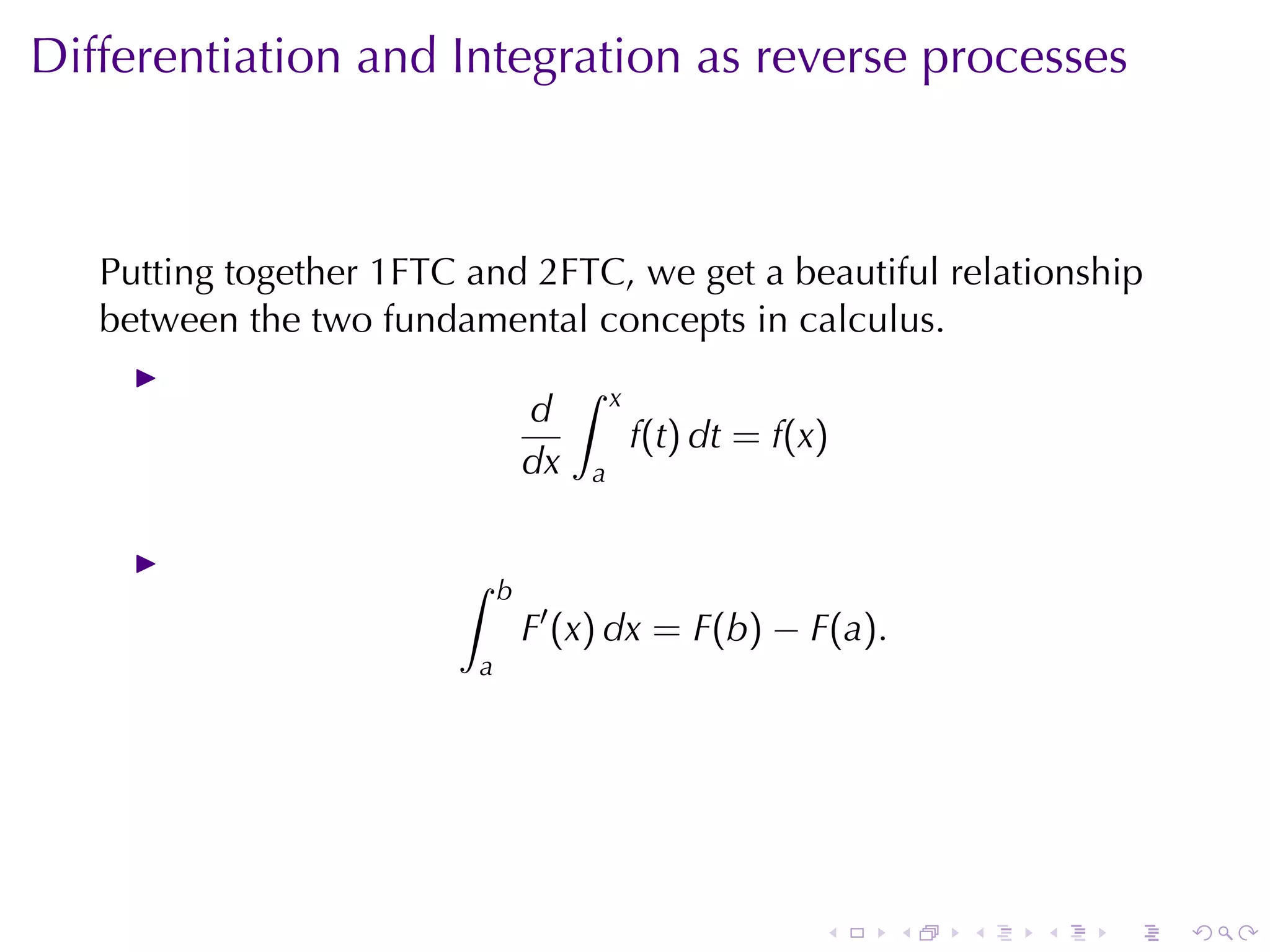

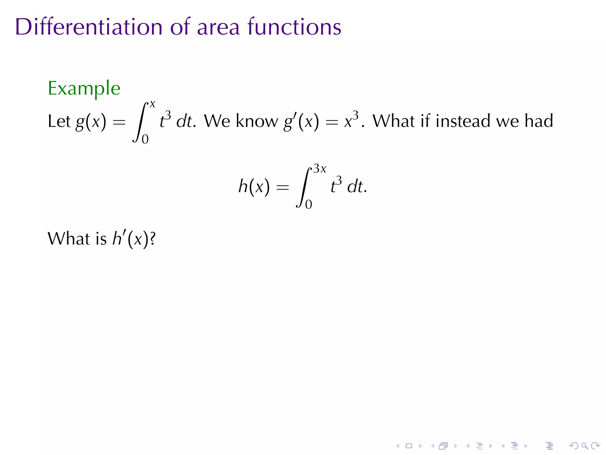

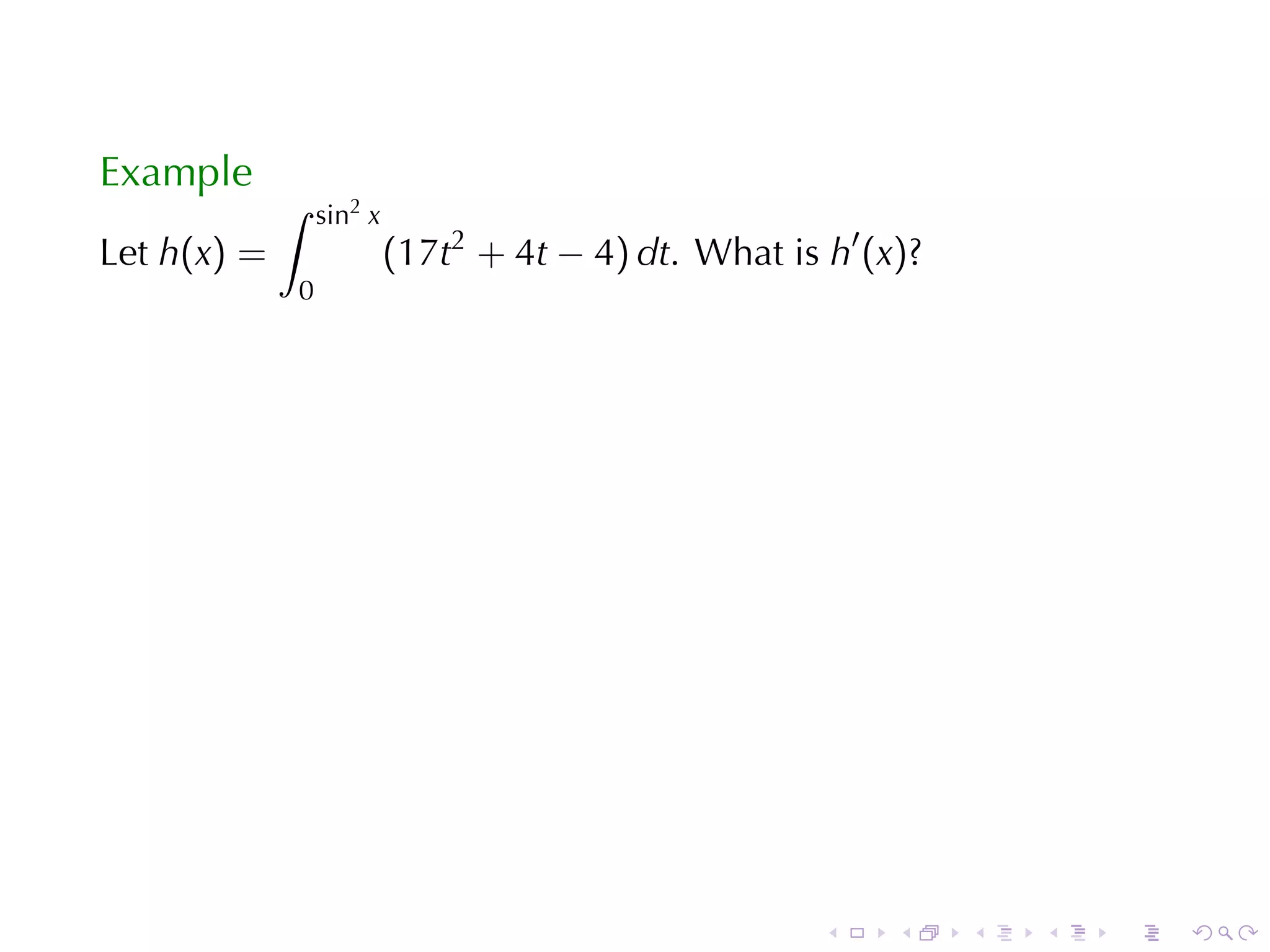


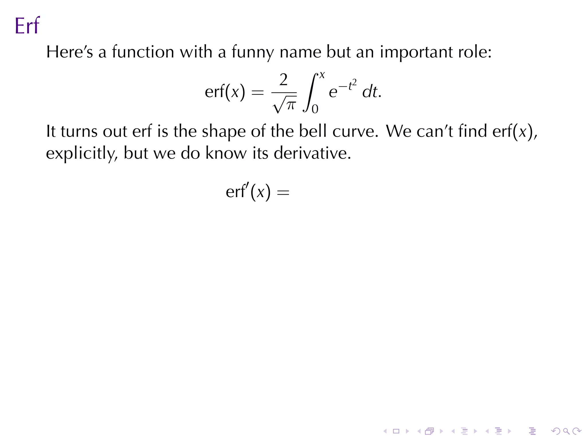
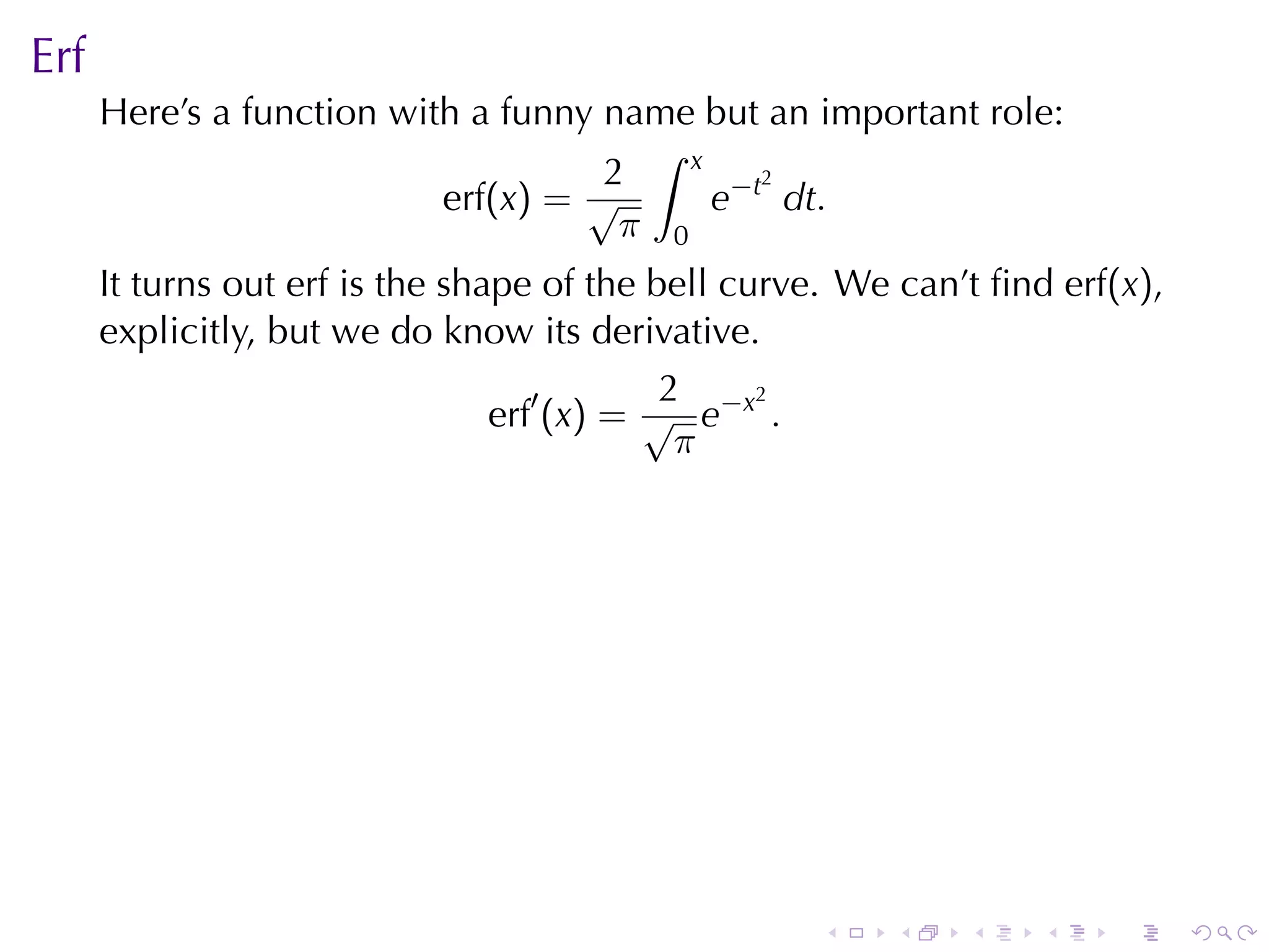
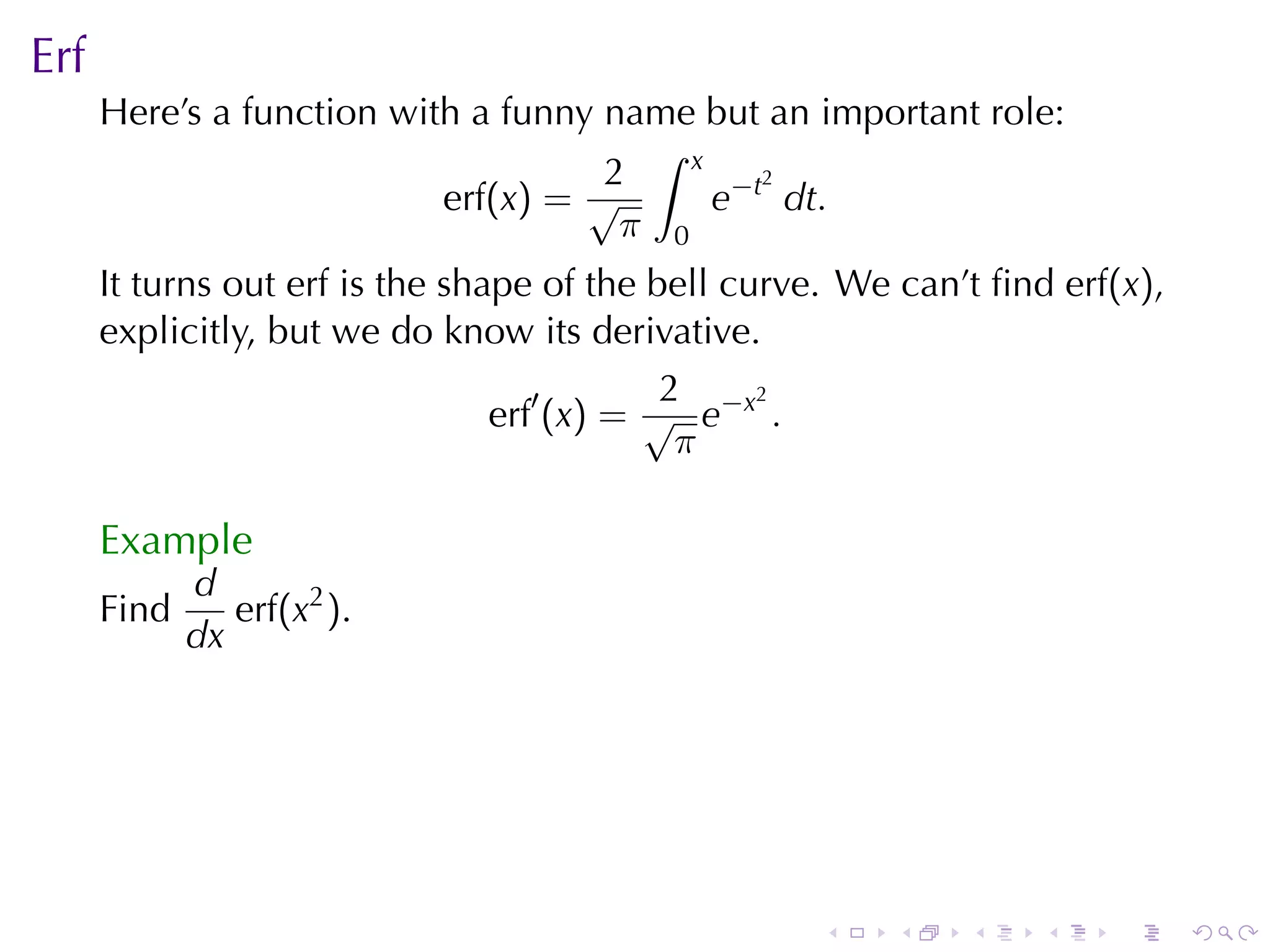
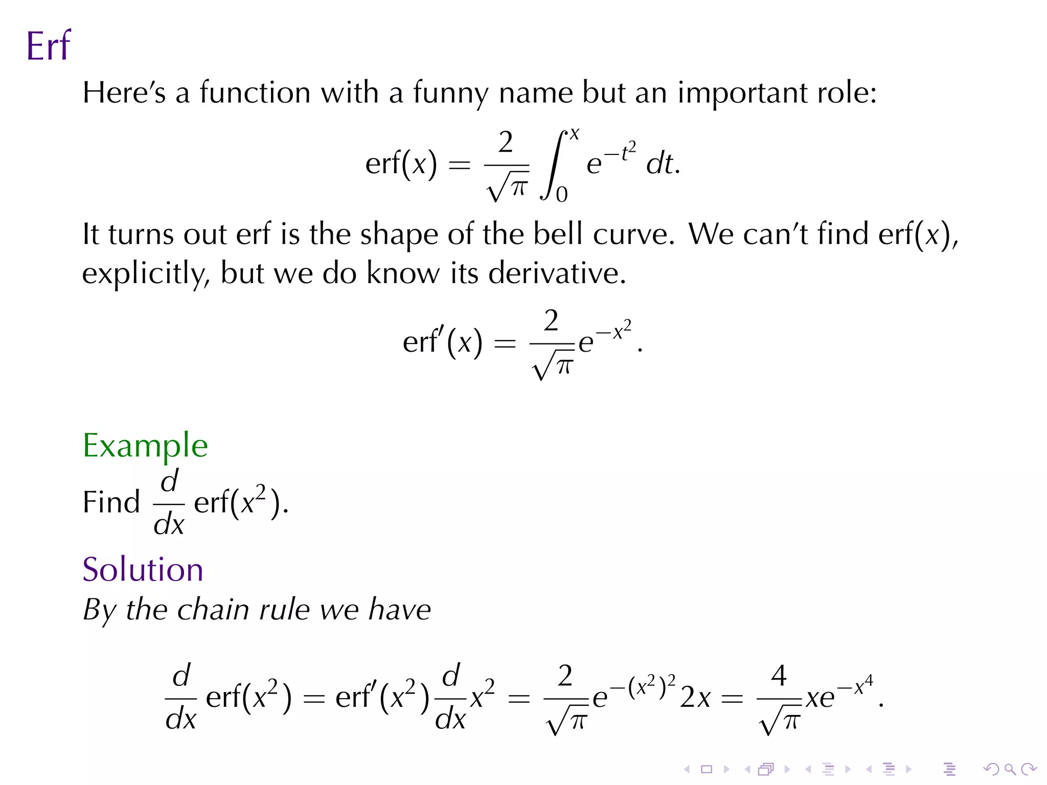
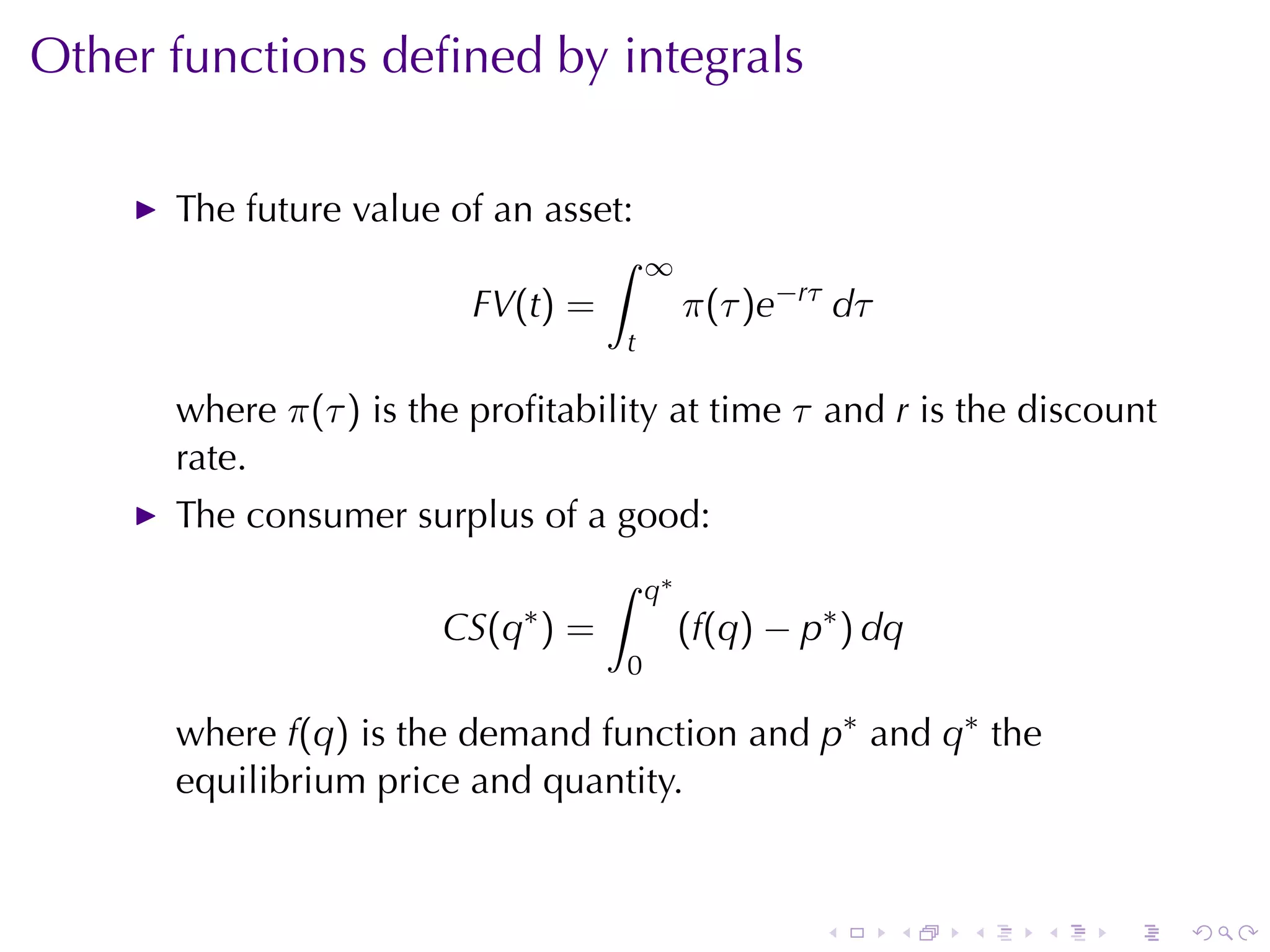

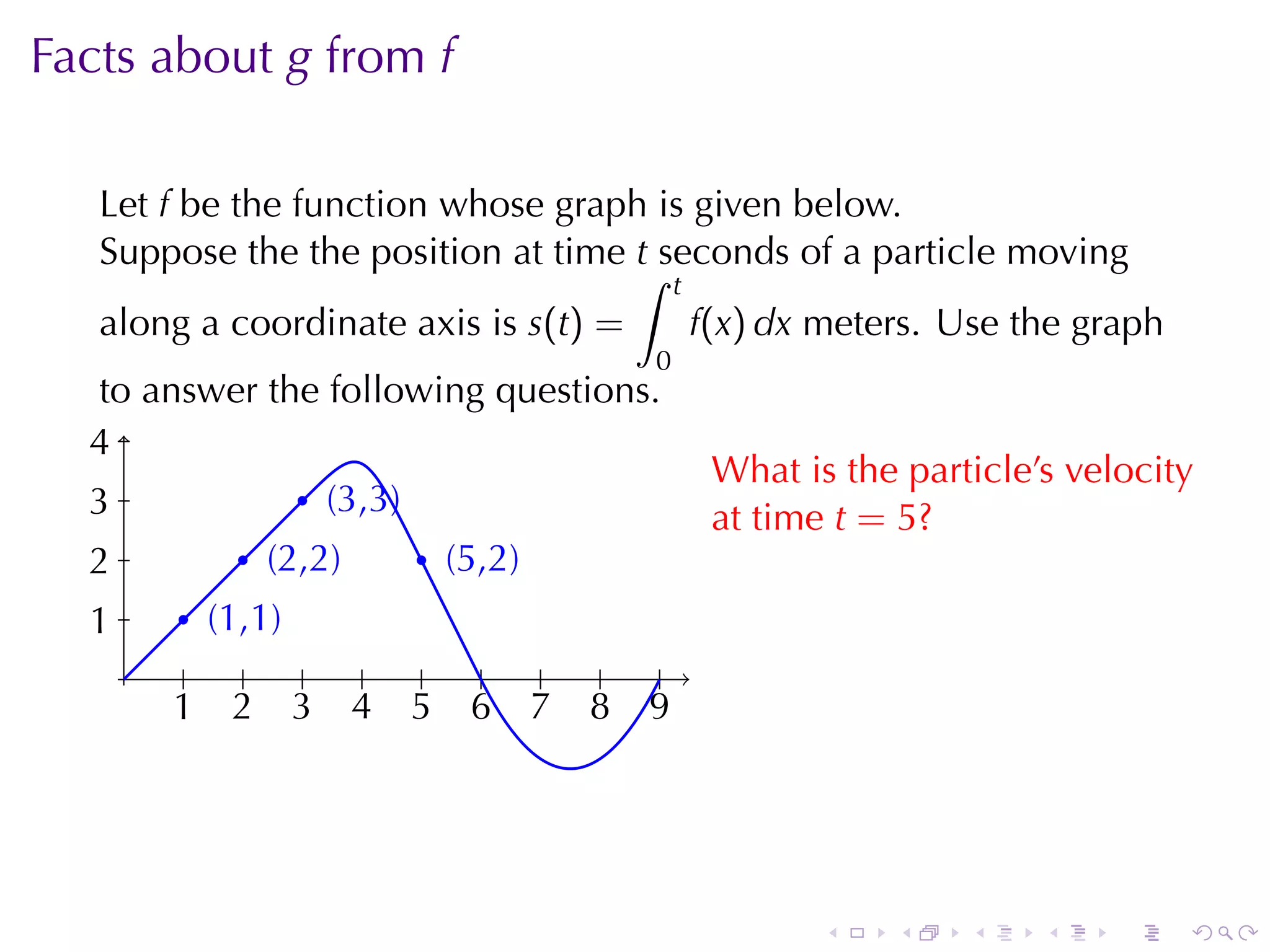

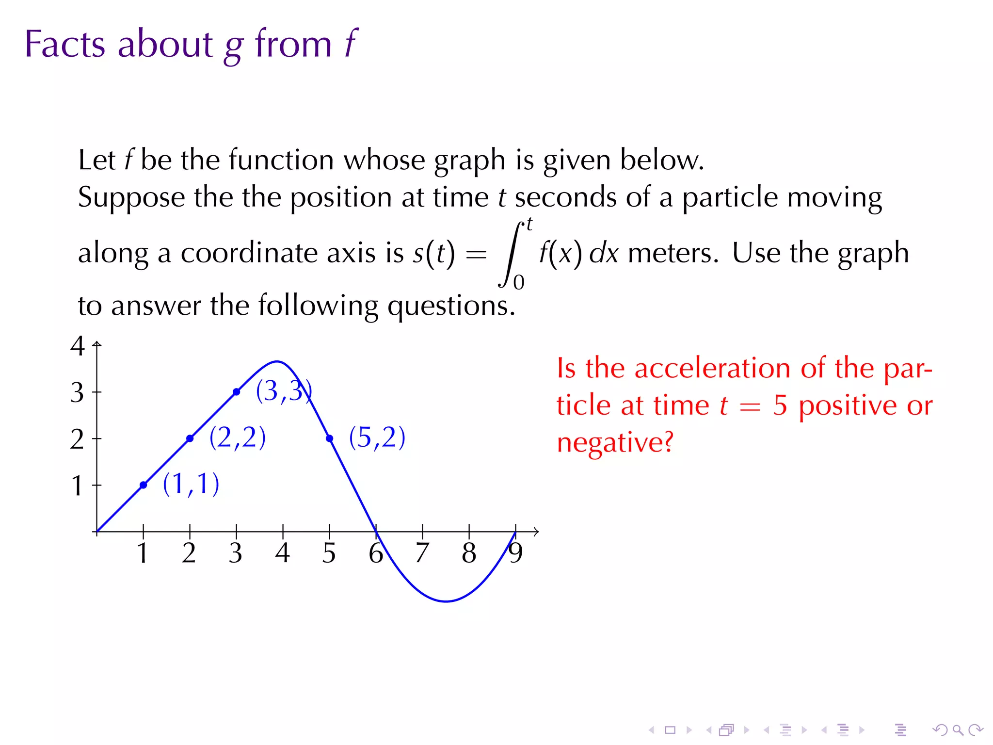
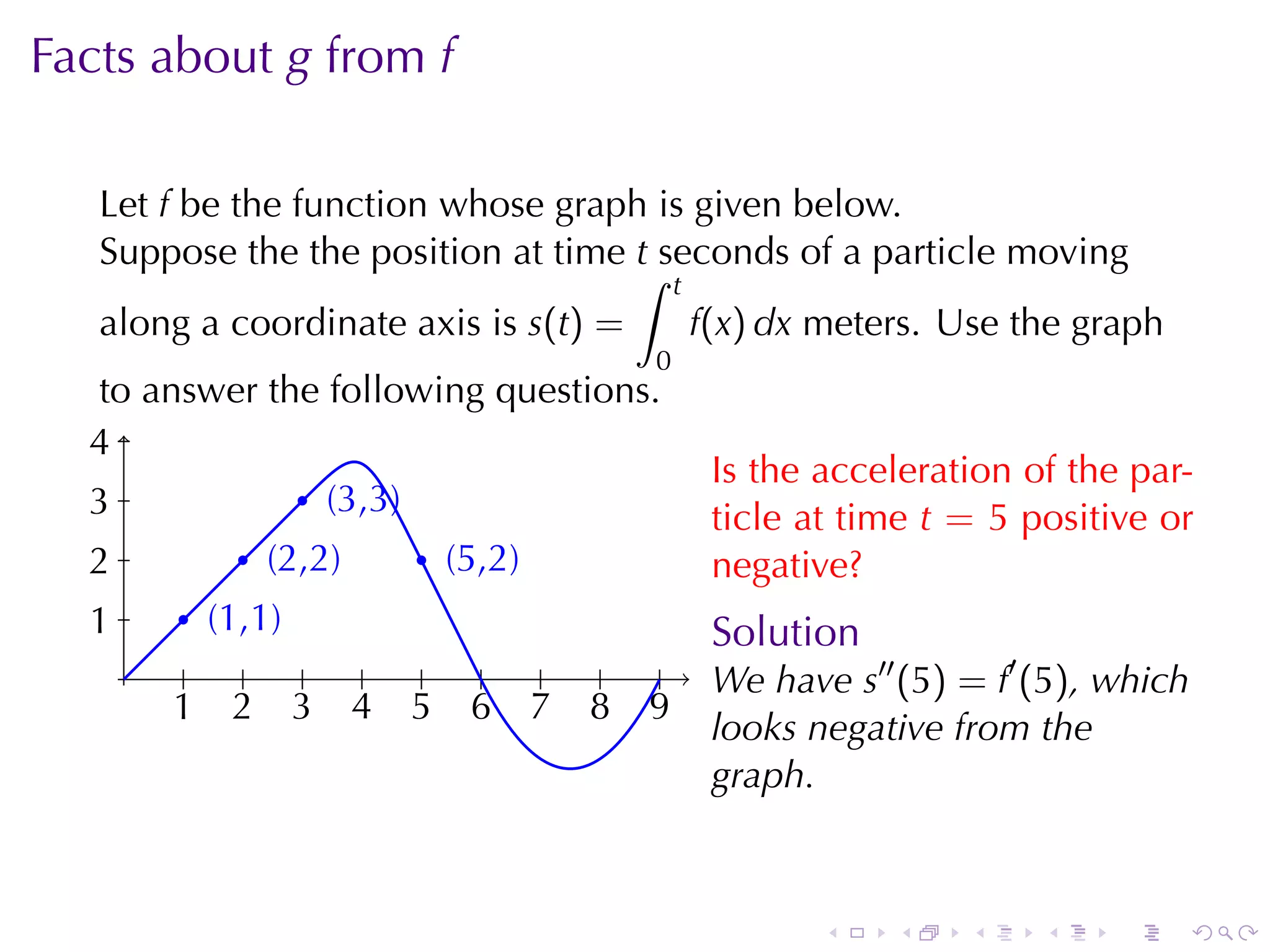
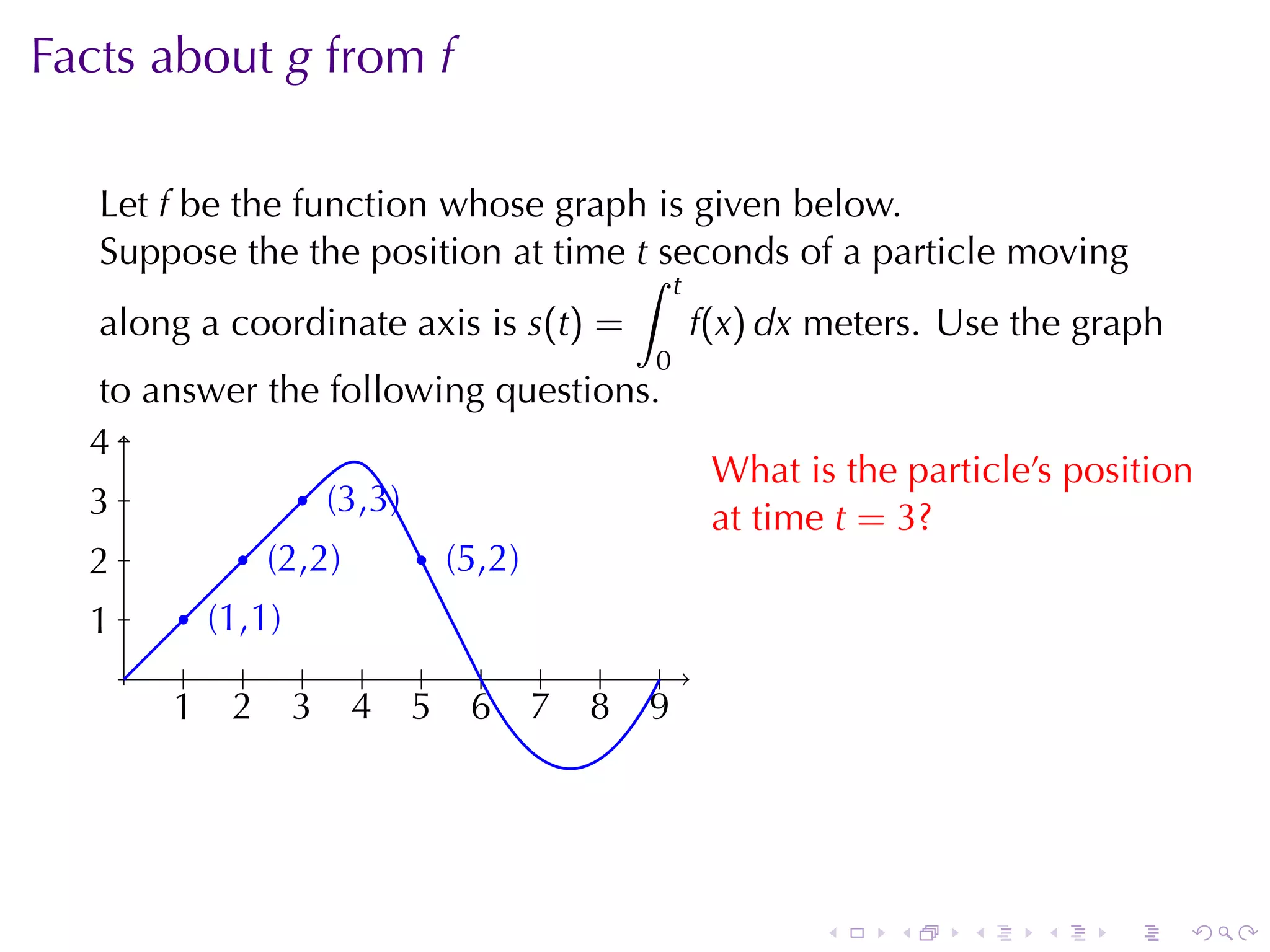

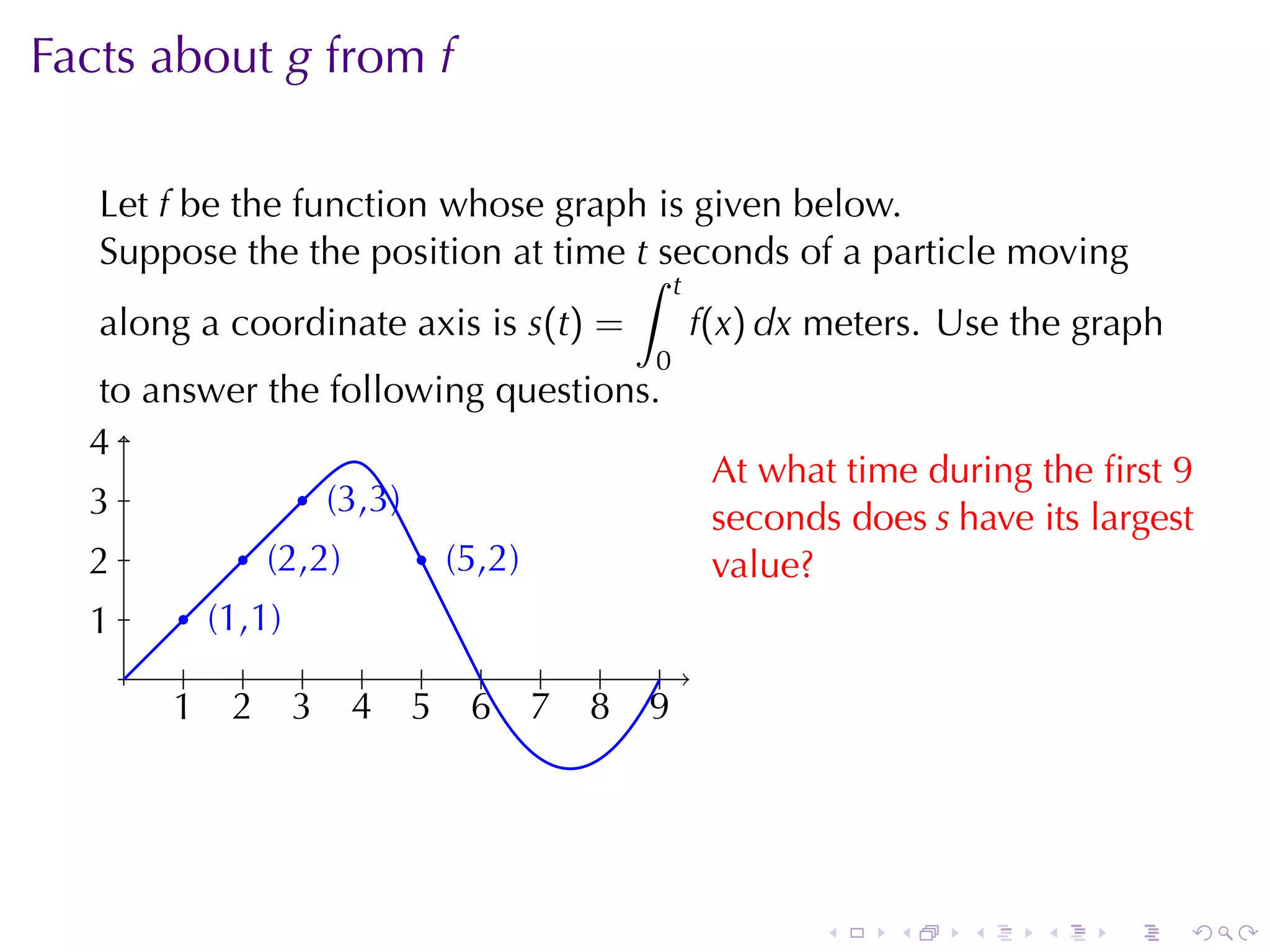

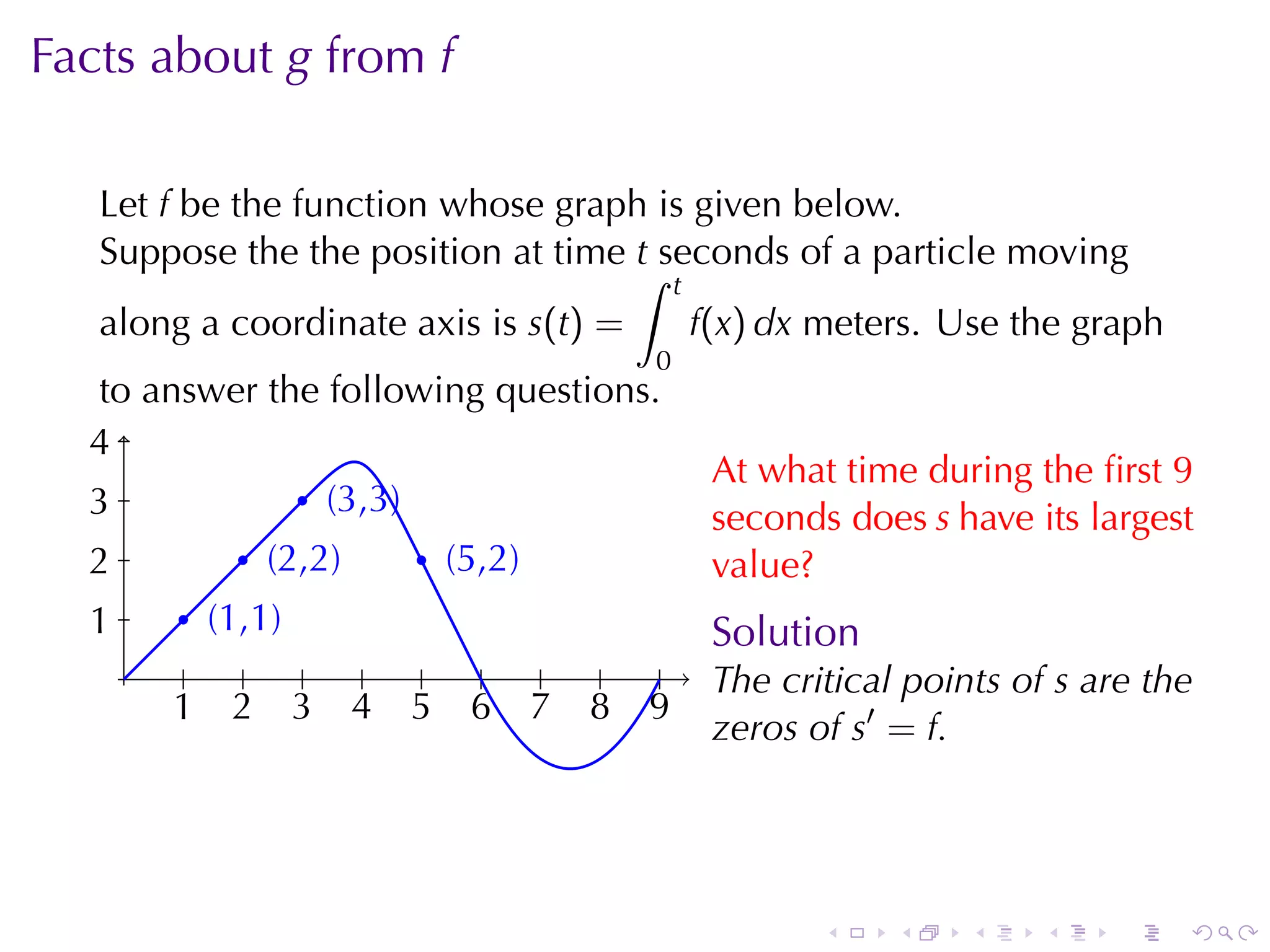


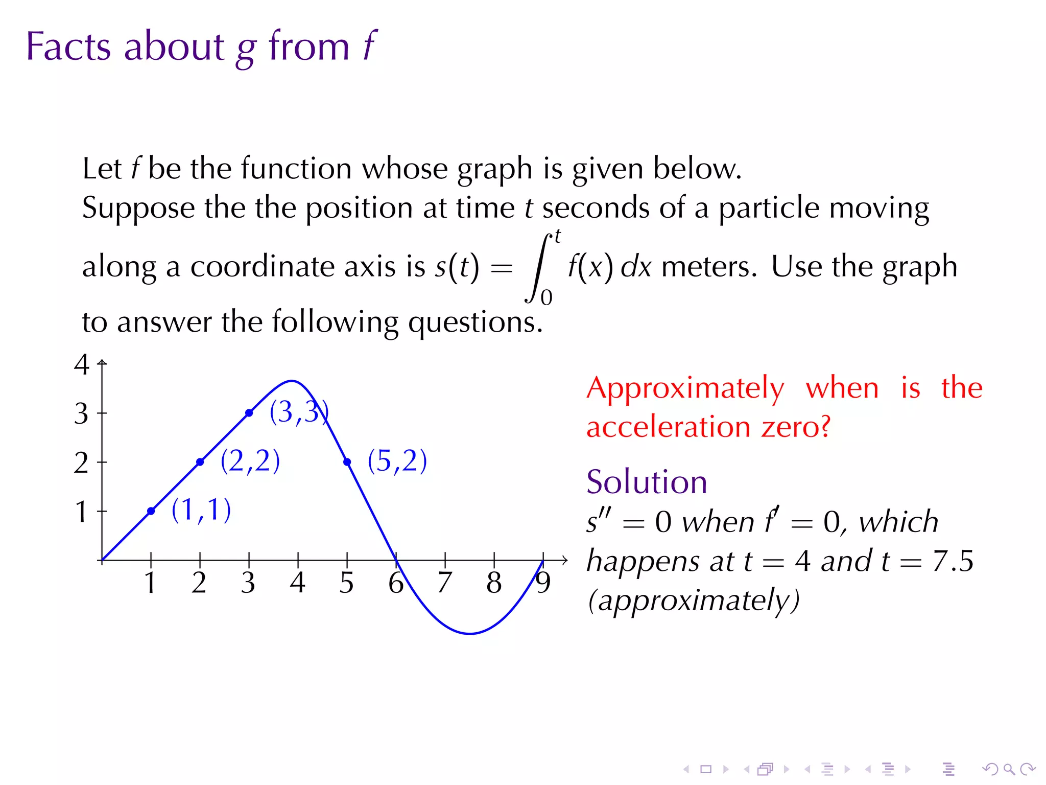

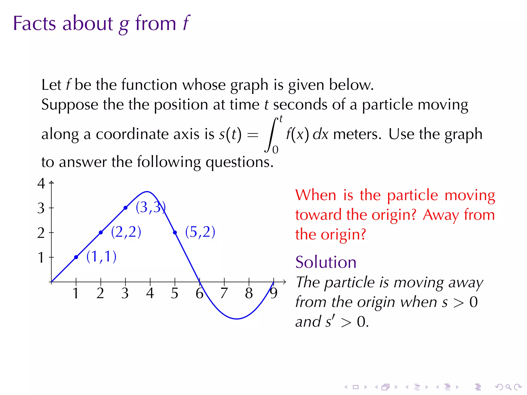

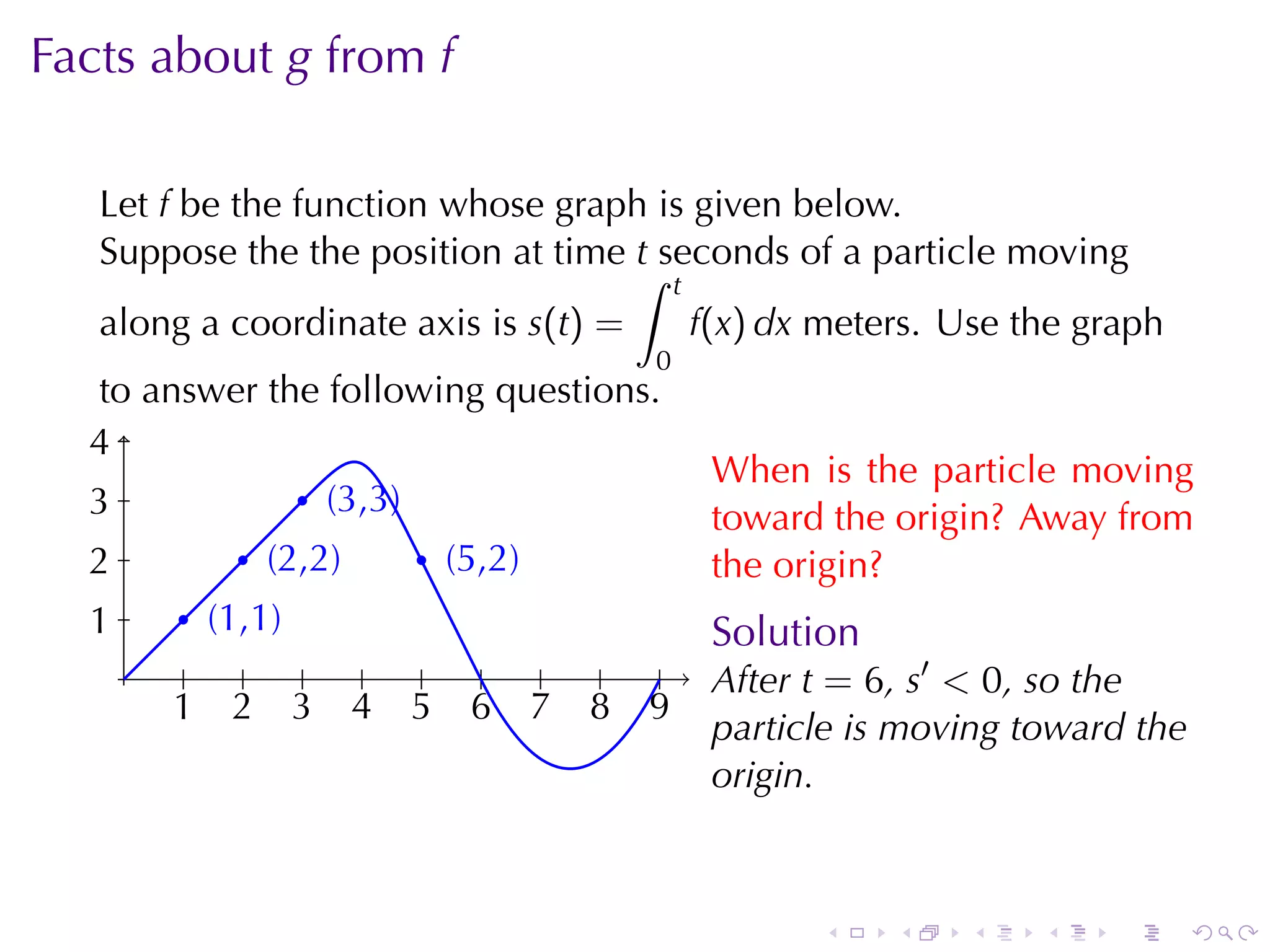


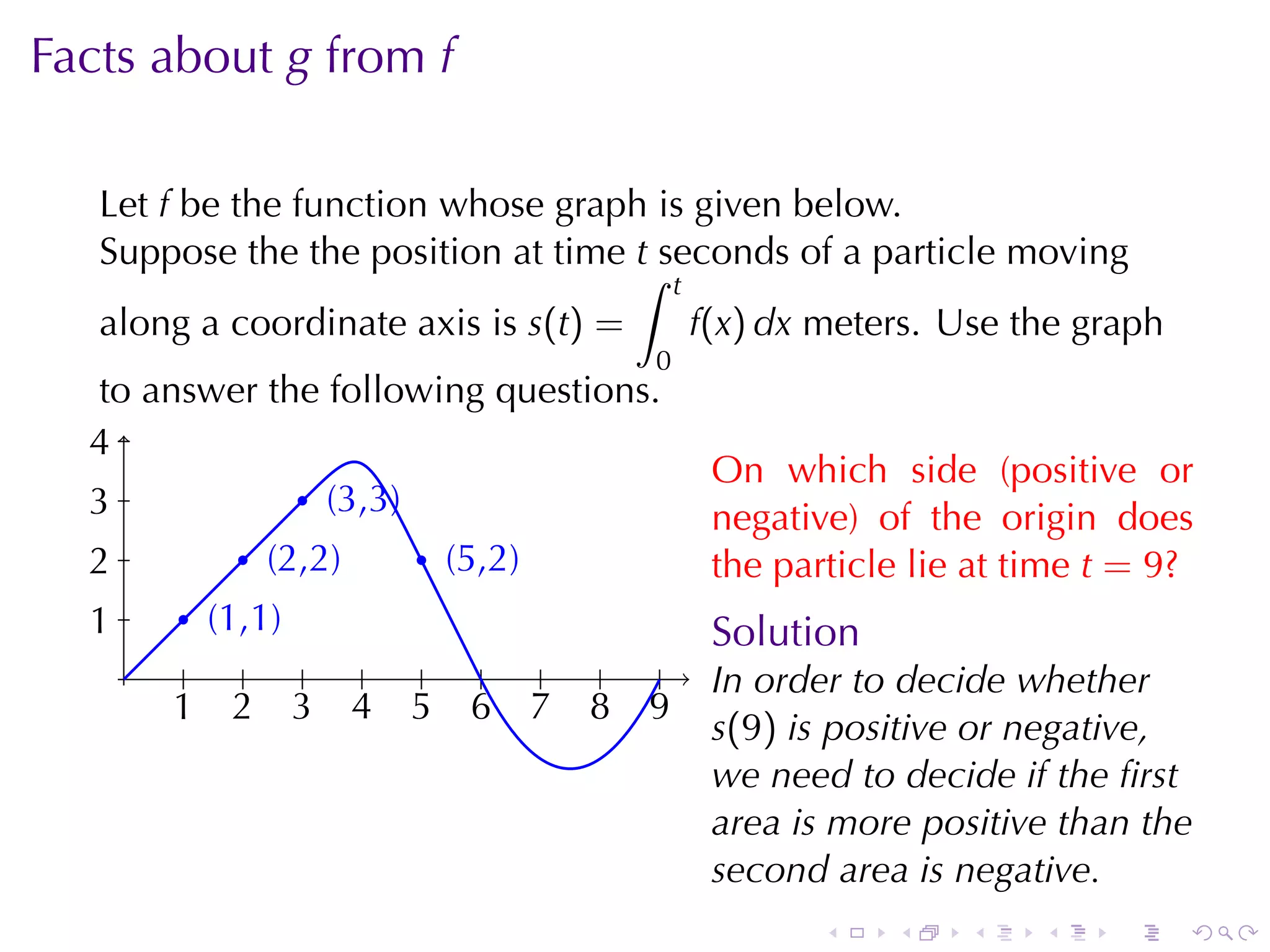


Section 5.4 discusses the fundamental theorem of calculus, which connects differentiation and integration, stating that the integral of a function's derivative over an interval represents the total change of the function. It outlines various theorems related to definite integrals, their geometric interpretations, and their applications in real-world contexts, such as calculating total change in velocity or cost. The section also emphasizes the importance of the first and second fundamental theorems in understanding the relationship between a function and its integral.