The document outlines statistical methods for decision-making, covering topics such as sampling, descriptive statistics, probability basics, and hypothesis testing. Key elements discussed include types of data, measures of central tendency and dispersion, as well as advanced concepts like covariance and coefficient of correlation. Overall, it serves as a comprehensive guide for understanding and applying statistical techniques in various contexts.

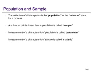
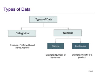
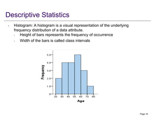
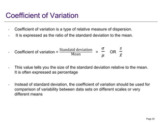
1. Statistical Methods for
Decision Making
Page 1

2. Agenda
• Sampling
• Basic Descriptive Statistics
• Probability basics, Bayes Theorem
• Probability distributions
• Sampling Distribution
• Interval Estimation and Hypothesis Testing
• Introduction to Linear Regression
Page 2

3. Descriptive Statistics
SMDM
Page 3

4. Agenda
• Population and Sample
• Data Collection
• Types of data
• Measures of central tendence
• Measures of dispersion
• Covariance and Coefficient of correlation
Page 4

5. Population and Sample
• The collection of all data points is the “population” or the “universe” data
for a process
• A subset of points drawn from a population is called “sample”
• Measurement of a characteristic of population is called “parameter”
• Measurement of a characteristic of sample is called “statistic”
Page 5

6. Data Collection – Data sources
• Primary vs Secondary data sources
• Internal vs External data sources
Page 6

7. Data Collection
• Observation
• Questionnaires and Surveys
• Interviews
etc
Page 7

8. Data Collection - Sampling
• Non-probability sampling: Selection is not statistically random. E.g. based
on judgement or convenience.
• Probability sampling
• Random sampling - Every item has equal chance of being selected
• Sampling without replacement
• Samling with replacement
• Stratified random sampling: Select randomly from predefined subgroups (strata)
• Cluster sampling – Sampling from naturally occurring clusters, e.g. cities.
• Systematic sampling – Divide into n groups containing k items. Randomly select
from first k items. Then select every kth item.
Page 8

9. Types of Data
Page 9
Example: Number of
items sold
Example: Weight of a
product
Example: Preferred brand
name, Gender
Types of Data
Categorical Numeric

10. Measurement Scale
Nominal data does not have order. For
example: gender
Ordinal data has a meaningful order.
For example: appraisal rating
Page 10
Interval example: Temperature in
Celsius.
Ratio example: Cost of an item
Measurement Scale
Categorical (Qualitative) Numeric (Quantitative)

11. Descriptive Statistics
• Central Tendency
• Mean: Arithmetic mean of numbers. Add the observations and divide by
count of the observations. Mean is affected by extreme values
• Median: When observations are sorted in ascending order, the middle
observation is median. If we have n observations, the (n+1)/2 th
observation is median. The median can be an observation or between
two observations
• Mode: Mode is the most frequently occurring data point in a data set
Page 11

12. Descriptive Statistics
• Range: It is the difference between the maximum and minimum values in a
data set. Affected by extreme values
• Inter Quartile Range (IQR) – IQR is the distance between the first and the
third quartile.
• First quartile (Q1) has 25% observation lower than it. (i.e. 25th
percentile)
• Third quartile (Q3) has 75% observation lower than it
• Median is also called second quartile (Q2)
• Variance is measured as the average of sum of squared difference
between each data point (represented by xi) and the mean represented by
Page 12
n
Σ (xi - ҧ
𝑥)2
i=1
------------
n - 1
N
Σ (xi - )2
i=1
------------
N
Unbiased
formula

13. Descriptive Statistics
• Standard deviation is one of the most popular measure of spread. It is the
square root of the variance.
Page 13
n
Σ (xi - ҧ
𝑥)2
i=1
------------
n - 1
N
Σ (xi - )2
i=1
------------
N Unbiased
formula

14. Descriptive Statistics
• Listing of Minimum, 1st quartile, Median, 3rd Quartile and Maximum is also called
“five number summary”
• Boxplot: A boxplot is a standardized way of displaying the distribution of data based
on a five-number summary (“minimum”, first quartile (Q1), median, third quartile
(Q3), and “maximum”).
• The box is drawn from Q1 to Q3
• Each whisker can extend maximum of (1.5 * IQR) beyond Q1 and Q3
• Any points beyond whisker, called outliers, are also plotted
Page 14

15. Discussion
• How to interpret the following
Page 15
OR
B
A
A B

16. Descriptive Statistics
• Histogram: A histogram is a visual representation of the underlying
frequency distribution of a data attribute.
• Height of bars represents the frequency of occurrence
• Width of the bars is called class intervals
Page 16

17. Skewness
• A measure of the asymmetry of distribution of data
• Types of Skewness:
• Positive Skew (Right Skew): Tail on the right side is longer.
• Negative Skew (Left Skew): Tail on the left side is longer.
• Symmetrical Distribution: Skewness ≈ 0.
Page 17
Image credit: https://www.analyticsvidhya.com/blog/2020/07/what-is-skewness-statistics/

18. Kurtosis
• A measure of “tailedness” or “peakedness” of a data
• Note: Additional information:
• Mesokurtic: Normal distribution. Excess Kurtosis ≈ 0.
• Leptokurtic: Peaked distribution with fat tails. Excess Kurtosis > 0.
• Platykurtic: Flat distribution with thin tails. Excess Kurtosis < 0.
Page 18

19. Coefficient of Variation
Comparing dispersion – food for thought
• Following is the performance of two factories in terms number of parts
produced per day
Factory 1: Standard deviation 10
Factory 2: Standard deviation 12
What is the observation?
Possible answer: it appears that the factory-2 has more variation in
output (note: this may not a correct answer)
Page 19

20. Coefficient of Variation
• Coefficient of variation is a type of relative measure of dispersion.
• It is expressed as the ratio of the standard deviation to the mean.
• Coefficient of variation =
Standatd deviation
Mean
=
𝜎
𝜇
OR
𝑠
ҧ
𝑥
• This value tells you the size of the standard deviation relative to the mean.
It is often expressed as percentage
• Instead of standard deviation, the coefficient of variation should be used for
comparison of variability between data sets on different scales or very
different means
Page 20

21. Coefficient of Variation
• Following is the performance of two factories in terms number of parts produced per
day
Factory 1: Standard deviation = 10
Factory 2: Standard deviation = 12
Factory 1: Mean = 100
Factory 2: Mean = 200
Factory 1: Coefficient of variation = 10/100 = 0.1 = 10%
Factory 2: Coefficient of variation = 12/200 = 0.06 = 6%
Now, what is the observation?
Factory-2 standard deviation is 6% of it’s mean while Factory-1 standard
deviation is 10% of it’s mean. So relatively, Factory-1 has more variation in
output
Page 21

22. Covariance
• Covariance measures the joint variability between two numerical variables
(X and Y).
• Covariance is calculated as
• Covariance measures the extent to which two variables vary linearly
• It reveals whether two variables move in the same or opposite directions.
• The larger the X and Y values, the larger the covariance. A value doesn’t
tell us exactly how strong that relationship is
Page 22

23. Covariance
• The sign of covariance reveals whether two variables move in the same or
opposite directions.
• The larger the X and Y values, the larger the covariance. The values of
Covariance is not range bound. Covariance value doesn’t indicate how
strong that relationship is
Image: https://www.allmath.com/covariance.php
Page 23
Positive
covariance
Negative
covariance
Near Zero
covariance
Positive
covariance
Negative
covariance

24. Coefficient of Correlation
• Coefficient of correlation, denoted as ‘r’ as calculated as:
• Its value can range between -1 to +1
• The sign of coefficient of correlation tell the direction of relation
• The value tells the measures the strength of a linear relationship between
two variables (X and Y)
• Note that the coefficient of correlation does not indicate causality
Page 24

25. Coefficient of Correlation
• A value closer to +1 indicates a strong positive (direct) relationship while a
value closer to -1 indicates a strong negative (inverse) relationship
• A value close to zero indicates no linear relationship
Page 25

26. Coefficient of Correlation
• Note that the coefficient of correlation does not indicate causality
Credit: https://xkcd.com/552/
Page 26

27. Thank you!
Page 27