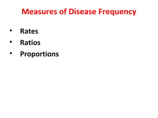
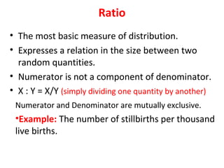
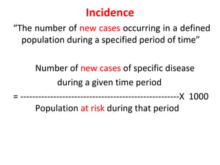
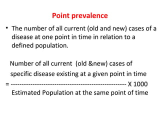
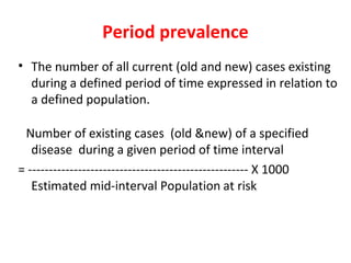
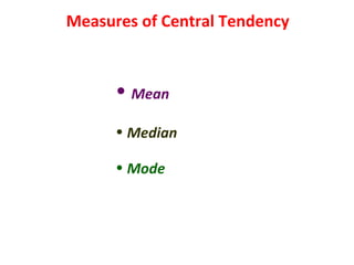
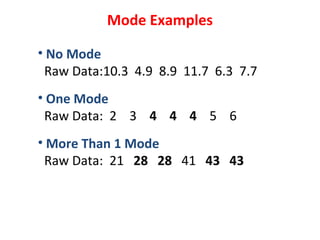
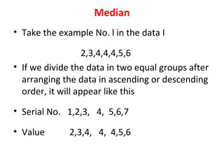
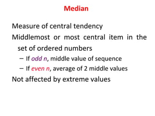
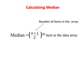
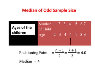
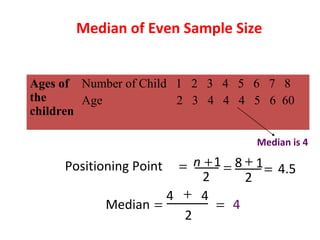
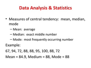
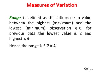
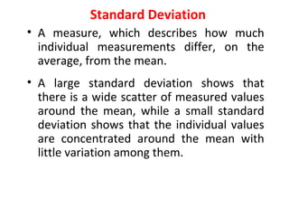
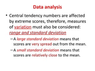
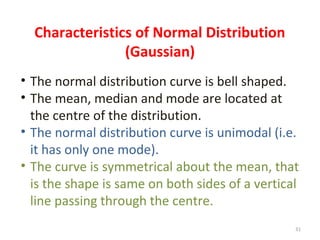
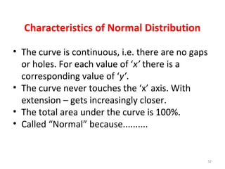
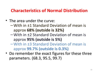
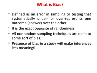
Measures of disease frequency include rates, ratios, and proportions. A ratio expresses the relation between two quantities where the numerator is not part of the denominator. A proportion indicates the relation of a part to the whole, with the numerator included in the denominator. A rate measures the occurrence of an event in a population during a time period. Other concepts discussed include incidence, prevalence, measures of central tendency (mean, median, mode), and measures of variation (range, standard deviation). Factors that can affect study outcomes include various types of biases such as selection, response, information, and confounding variables.

1. Measures of Disease Frequency
• Rates
• Ratios
• Proportions

2. Ratio
• The most basic measure of distribution.
• Expresses a relation in the size between two
random quantities.
• Numerator is not a component of denominator.
• X : Y = X/Y (simply dividing one quantity by another)
Numerator and Denominator are mutually exclusive.
•Example: The number of stillbirths per thousand
live births.

3. Proportion
• A proportion is a ratio which indicates the
relation in magnitude of a part to the whole.
• Numerator is always included in the
denominator.
• Usually expressed as percentage.
• For example: the proportion of women over
the age of 50 who have had a hysterectomy, or
the number of fetal deaths out of the total
number of births (live births plus fetal deaths).

4. Rate
• 500 deaths from motor vehicle accidents in city
A during 1985.
• For comparison between City A and City B
calculate Rate.
• Rate measures the occurrence of some
particular event in a population during a given
time period.
• For example, the number of newly diagnosed
cases of breast cancer per 100,000 women
during a given year.

5. A Proportion with specifications of Time
• Distinct Relationship between Numerator &
Denominator.
• Death Rate: CDR, IMR, MMR.
• Specific Rate: Disease specific, age – group
specific, specific time periods.
• Standardized rates: By direct method and
indirect method.

6. Incidence
“The number of new cases occurring in a defined
population during a specified period of time”
Number of new cases of specific disease
during a given time period
= -----------------------------------------------------X 1000
Population at risk during that period

7. 7
Issues in the Calculation of Incidence
For any measure of disease frequency,
precise definition of the denominator is
essential for both accuracy and clarity. This is
a particular concern in the calculation of
incidence. The denominator of a measure of
incidence should include only those who are
considered "at risk" of developing the
disease.

8. 8
Special Types of Incidence Rates
Morbidity Rate: the incidence rate of non fatal cases in
the total population at risk during a specified period of
time, e.g., the morbidity rate of TB in the US in 1982 was
calculated by dividing the number of nonfatal cases
newly reported during that year by the total US midyear
population.
Total no of nonfatal cases of TB = 25,520/ 231,534,000
Mid year Population
= 11.0 per 100,000 population

9. • Expresses the incidence of deaths in a
particular population during a specific period of
time.
• Calculated by dividing the number of fatalities
during that period by the total population.
Mortality Rate

10. Prevalence
• All current cases (old & new) existing at a
given point of time, or over a period of time in
a given population.
• Definition: the total number of all individuals
who have an attribute or disease at a
particular time divided by the population at
risk of having the attribute or disease at this
point in time or midway through the period

11. Point prevalence
• The number of all current (old and new) cases of a
disease at one point in time in relation to a
defined population.
Number of all current (old &new) cases of
specific disease existing at a given point in time
= ----------------------------------------------------- X 1000
Estimated Population at the same point of time

12. Period prevalence
• The number of all current (old and new) cases existing
during a defined period of time expressed in relation to
a defined population.
Number of existing cases (old &new) of a specified
disease during a given period of time interval
= ----------------------------------------------------- X 1000
Estimated mid-interval Population at risk

13. Measures of Central Tendency
• Mean
• Median
• Mode

14. • If the whole sheets of information are
presented to anybody he/she cannot make any
meaning out of it and if the question is such
that you should present the gist of information
in a single word, then it becomes more
difficult.
• History tells us that this question was
answered by giving the average value of the
data.
• Take the example of the following data of ages
of the children:
2,3,4,4,4,5,6 -------- (Data I)

15. Mean
Also known as the AVERAGE. It Is
calculated by totaling the results of all the
observations and dividing by the total
number of observations. Note that the
mean can only be calculated for
numerical data.

16. Mode
• Scientists after a lot of discussion gave
solution to the problem by recommending
that the most frequently occurring value (most
repeated) should be taken as representative
because it will involve most of the people and
thus most of the people will be benefited and
it was termed as MODE. (TB, Malaria, Typhoid)

17. Mode Examples
• No Mode
Raw Data:10.3 4.9 8.9 11.7 6.3 7.7
• One Mode
Raw Data: 2 3 4 4 4 5 6
• More Than 1 Mode
Raw Data: 21 28 28 41 43 43

18. Median
• Take the example No. l in the data I
2,3,4,4,4,5,6
• If we divide the data in two equal groups after
arranging the data in ascending or descending
order, it will appear like this
• Serial No. 1,2,3, 4, 5,6,7
• Value 2,3,4, 4, 4,5,6

19. Median
Measure of central tendency
Middlemost or most central item in the
set of ordered numbers
– If odd n, middle value of sequence
– If even n, average of 2 middle values
Not affected by extreme values

20. Calculating Median
Median = item in the data array( )thn + 1
2
Number of items in the array

21. Median of Odd Sample Size
Median
PositioningPoint
Median
=
+
=
+
=
=
n 1
2
7 1
2
4 0
4
.
Number 1 2 3 4 5 6 7
of Child
Age 2 3 4 4 4 5 6
Ages of the
children

22. Median of Even Sample Size
Median is 4
Positioning Point
Median
= + = +
=
=
+
=
n 1
2
8 1
2
4.5
4 4
2
4
Ages of
the
children
Number of Child 1 2 3 4 5 6 7 8
Age 2 3 4 4 4 5 6 60

23. Data Analysis & Statistics
• Measures of central tendency: mean, median,
mode
– Mean: average
– Median: exact middle number
– Mode: most frequently occurring number
Example:
67, 94, 72, 88, 88, 95, 100, 88, 72
Mean = 84.9, Medium = 88, Mode = 88

24. Range is defined as the difference in value
between the highest (maximum) and the
lowest (minimum) observation e.g. for
previous data the lowest value is 2 and
highest is 6
Hence the range is 6-2 = 4
Measures of Variation
Cont…

25. Standard Deviation
• A measure, which describes how much
individual measurements differ, on the
average, from the mean.
• A large standard deviation shows that
there is a wide scatter of measured values
around the mean, while a small standard
deviation shows that the individual values
are concentrated around the mean with
little variation among them.

26. Data analysis
• Central tendency numbers are affected
by extreme scores, therefore, measures
of variation must also be considered:
range and standard deviation
–A large standard deviation means that
scores are very spread out from the mean.
–A small standard deviation means that
scores are relatively close to the mean.

27. 27
Standard error of the mean
• When we draw a sample from study population and
compute its sample mean it is not likely to be
identical to the population mean. If we draw
another sample from same population and compute
its sample mean, this may also not be identical to
the first sample mean. It probably also differs from
the true mean of the total population from which
the sample was drawn this phenomenon is called
sampling variation.
• Standard error: gives an estimate of the degree to
which the sample mean varies from the population
mean and this measures is used to calculate
Confidence Interval.

28. 28
The Normal Distribution
• Many variables have a normal distribution.
This is a bell shaped curve with most of the
values clustered near the mean and a few
values out near the tails.

29. 29
• The normal distribution is symmetrical
around the mean. The mean, the median
and the mode of a normal distribution have
the same value.
• An important characteristic of a normally
distributed variable is that 95% of the
measurements have value which are
approximately within 2 standard deviations
(SD) of the mean.

30. 30
The Normal Distribution

31. Characteristics of Normal Distribution
(Gaussian)
• The normal distribution curve is bell shaped.
• The mean, median and mode are located at
the centre of the distribution.
• The normal distribution curve is unimodal (i.e.
it has only one mode).
• The curve is symmetrical about the mean, that
is the shape is same on both sides of a vertical
line passing through the centre.
31

32. Characteristics of Normal Distribution
• The curve is continuous, i.e. there are no gaps
or holes. For each value of ‘x’ there is a
corresponding value of ‘y’.
• The curve never touches the ‘x’ axis. With
extension – gets increasingly closer.
• The total area under the curve is 100%.
• Called “Normal” because..........
32

33. Characteristics of Normal Distribution
• The area under the curve:
–With in ±1 Standard Deviation of mean is
approx 68% (outside is 32%)
–With in ±2 Standard Deviation of mean is
approx 95% (outside is 5%)
–With in ±3 Standard Deviation of mean is
approx 99.7% (outside is 0.3%)
• Do remember the exact figures for these three
parameters. (68.3, 95.5, 99.7)
33

34. 34
Factors Affecting Study
Outcomes

35. What is Bias?
• Defined as an error in sampling or testing that
systematically under- or over-represents one
outcome (answer) over the other.
• It is the exact opposite of randomness.
• All nonrandom sampling techniques are open to
some sort of bias.
• Presence of bias in a study will make inferences
less meaningful.

36. Types of Biases
There are basically only three major types of
biases.
 Selection bias
 Response bias
 Information bias
All others are simply varieties of these three
types

37. Selection Bias
– Caused by nonrandom sampling, so that a
systematic difference is present between people
selected for the study and people not selected
for the study.
– Can be caused by convenience sampling, patient
referral patterns, survival differences or loss to
follow-up.
– An avoidable bias, if not eliminated, can ruin the
chances of acceptance or publication of the
study.

38. Response Bias
– a (selection) bias where respondents differ
systematically from non-respondents.
– For example, people with a certain disease (or
their relatives) are more likely to respond to oral
or written questions than normal people.
– More educated people are more likely to provide
answers and correct answers than less educated
or informed people.
– those who agree to be in a study may be in some
way different from those who refuse to
participate (Volunteers may be different from those who
are enlisted)

39. Information (Measurement) Bias
– a systematic difference between the measurements
(or information) recorded in different study groups.
– For example, in cohort studies, people with the risk
factor may be tested more frequently and carefully
than the control group. This is also called
‘surveillance’ bias or ‘diagnostic suspicion’ bias.

40. Interviewer Bias
• an interviewer’s knowledge may influence the
structure of questions and the manner of
presentation, which may influence responses
• Interviewer’s IQ may also influence in
understanding the responses
• Observer Bias – observers may have
preconceived expectations of what they
should find in an examination

41. Recall Bias
– a type of information bias, when people with a
certain condition are more likely to remember
exposure to the risk factor under study than the
control group. It can occur easily in case-control
or cross-sectional studies, but not in cohort
studies. (those with a particular outcome or exposure may
remember events more clearly or amplify their recollections)
– For example parents of children with cancer may
‘remember’ more information about details of
risk factors and their exposure to them, than
parents of control children with identical
exposure rates.

42. Attrition Bias (Loss to follow-up)
– Attrition is a reduction in the number of
patients who remain in the study (patient drop
out).
– This results in an attrition bias when the
patients who drop-out of the study are
systematically different from those who remain
in and complete the study.
– It can occur in clinical trials and in cohort
studies.

43. Types of Variables
Dependent Variables Independent
Variable
Confounding Variable

44. Clearly state which variable is the dependent
and which are the independent ones.
From the statement of the problem and the
objectives of the study, determine whether a
variable is dependent or independent.
When designing a study

45. Certain variables may produce changes in the
DV which are mistakenly interpreted as
representing effects of the IV. When this
happens, the variable is called a confounding
variable because its effects are confused with IV
effects.
Definition
A variable that is associated with the problem
and with a possible cause of the problem is a
potential Confounding Variable.

46. A confounding variable may either strengthen or weaken
the apparent relationship between the problem and a
possible cause.
Cause Effect/outcome
(independent variable) (dependent variable)
Other factors
(confounding variables)

47. 47
Confounding can be thought of as mixing of the
effect of the exposure under study on the
disease with that of an extraneous factor.
This external factor or variable must be
associated with the exposure and, independent
of the exposure must be a risk factor for the
disease.
Confounding

48. 48
Example of confounding
Smoking MI
age

49. 49
Table 1. Relation of Myocardial infarction
(MI)to Recent Oral Contraceptive (OC) Use
MI Control Estimated
relative risk
OC
Yes 29 135 =1.68
No 205 1607
Total 234 1742

50. 50
Table: Age -specific Relation of Myocardial infarction
(MI) to recent Oral Contraceptive (OC) Use
Age (yrs) Recent
OC use
MI Controls Estimated age-
Specific relative risk
25 – 29 Yes
No
4
2
62
224
7.2
30 – 34 Yes
No
9
12
33
390
8.9
35 – 39 Yes
No
4
33
26
330
1.5
40 – 44 Yes
No
6
65
9
362
3.7
45 – 49 Yes
No
6
93
5
301
3.9
Total 234 1742

51. 51
Confounding can be controlled in study design
through:
 Restriction
Matching exposure
 Randomization
Confounding can be controlled in analysis
through:
 Stratification
 Multivariate analysis

52. Estimation
The process of using sample information
to draw conclusion about the value of a
population parameter is known as
estimation.

53. • A point estimate is a specific numerical value
estimate of a parameter.
• The best point estimate of the population mean
µ is the sample mean
• But how good is a point estimate?
• There is no way of knowing how close the point
estimate is to the population mean
• Statisticians prefer another type of estimate
called an interval estimate
Point Estimate
X

54. 54
Interval Estimate
• An interval estimate of a parameter is an interval or a
range of values used to estimate the parameter
Confidence Level
 The confidence level of an interval estimate of a parameter
is the probability that the interval estimate will contain
the parameter
 Three commonly used confidence levels are 90%, 95%
and 99%
 If one desires to be more confident then the sample size
must be larger

55. What is Hypothesis?
• A testable theory, or statement of
belief used in evaluation of a population
parameter of interest e.g. Mean or
proportion.
• Prediction of the relationship
between one or more factors and the
problem under study, which can be
tested.

56. • Suppose a study is being conducted to answer
questions about difference between two regimens
for the management of diarrhea in children:
– The sugar based modern ORS and
– The time-tested indigenous herbal solution made from
locally available herbs.
• One question that could be asked is:
"In the population is there a difference in overall
improvement (after three days of treatment)
between the ORS and the herbal solution?"

57. • There could be only two answers to
this question:
• Yes
• No

58. Null Hypothesis
"There is no difference between the 2
regimens in term of improvement” (null
hypothesis).
A null hypothesis is usually a statement that
there is no difference between groups or that
one factor is not dependent on another and
corresponds to the No answer.

59. Alternative Hypothesis
• "There is a difference in terms of improvement
achieved by a three days treatment with the ORS and
that of the herbal solution" (alternative hypothesis).
• Associated with the null hypothesis there is always
another hypothesis or implied statement concerning
the true relationship among the variables or
conditions under study if no is an implausible
answer. This statement is called the alternative
hypothesis and corresponds to the “Yes” answer.

60. Types of Alternate Hypothesis
o Directional
o Non Directional

61. Court Decision Guilty
Guilty  Wrong Decision
Correct Decision Alpha Error
(Type 1 error)
Wrong Decision Correct Decision
Not Guilty Beta Error 
(Type 2 error)
True Situation
Not Guilty
αα andand ββ errorerror

62. When we mistakenly reject the null when
indeed the null is true, then the type of wrong
decision is known as a Type I or Alpha error.
However when we mistakenly do not reject our
null when in fact it is false then we commit
another error known as the Type II or Beta
error.

63. P stands for probability.
• Probability of rejecting Ho Hypothesis
when it is true.
P – Value

64. P – Value
Also defined as
• Probability of falsely rejecting Ho
• Probability of finding the result by chance
alone
• Probability of committing Type I error or
Alpha error

65. The P value is a function of two factors:
•The magnitude of difference between
the groups.
•The size of the sample.

66. Steps in Hypothesis Testing
1. Statement of research question in terms of
statistical hypothesis (Null and alternate
hypothesis)
2. Selection of an appropriate level of
significance. The significance level is the risk
we are willing to take that a sample which
showed a difference was misleading. (5%
significance level means that we are ready to
take a 5% chance of wrong results).

67. 3. Choosing an appropriate statistics t test, z
test for continuous data, chi square for
proportions etc.
Test statistics is computed from the sample
data and is used to determine whether the null
hypothesis should be rejected or retained.
Test statistics generates p value
Steps in Hypothesis Testing

68. P value: Indicates the probability or likelihood of
obtaining a result at least as extreme as that
observed in a study by chance alone, assuming that
there is truly no association between exposure and
outcome under consideration.
By convention the p value is set at 0.05 level. Thus
any value of p less than or equal to 0.05 indicates
that there is at most a 5% probability of observing
an association as large or larger than that found in
the study due to chance alone given that there is no
association between exposure and outcome. If p
value>0.05 do not reject the null hypothesis .

69. 4. Performing calculations and obtaining p
value.
5. Drawing conclusions, rejecting null
hypothesis if the p value is less than the
set significance level.

70. SAMPLE SIZE ESTIMATIONSAMPLE SIZE ESTIMATION

71. Requirements
1 – the parameters (proportion or mean)
2 – the degree of precision (α)
3 – the desired confidence level (z)
4 – the estimated degree of variability of observation
(standard deviation)

72. Example 1
Estimating The Sample Size
Question: What Parameter do you want to
study?
Answer: I want to estimate the average increase
in body weights of Infant Rats, given Treatment
A within a certain period of time.

73. Q 2 What is expected Std Dev
• S.D. = 20 gm
• Q 3: How much error is tolerable?
• ANSWER A : 10 gm OR less
• ANSWER B : 5% of mean
• Q 4: What is mean?
• ANSWER: Mean = 100 gm
• How confident do you want to be ?
• 95% = {Z}

74. IN CASE OF ANS a TO Q3
Sample Size will be
n = (Z)2
(S)2
e2
=1.96 x 1.96 x 20 x 20
= 16
10 x 10

75. IN CASE OF ANS b TO Q3
Sample Size will be
n = (Z)2
(S)2
e2
= 1.96 x 1.96 x 20 x 20 = 62
5X5

76. 76
Sample size estimationSample size estimation:
n = Z 2 Pq
e
Z = 1.96 deviant error for .05
P = Prevalence
q = 1 - P
e = Tolerance error (5)
(.01 ---> .1)

77. In Case of Prevalence as 20%
Sample Size will be
n = Z2
x p x q
e2
n = 1.96 x 1.96 x 20 x 80 = 246
5 x5

78. 1. Type of study.
2. Magnitude of the outcome of interest derived
from previous studies.
3. Type of statistical analysis
required (comparing means or proportions).
4. Level of significance / Power.
Sample size calculations depend on:

79. 1. The prevalence of the condition/
attribute of interest.
2. Level of confidence.
3. Margin of error.
Sample size for single proportion depends on:

80. Example of Sample size calculation for single
proportion
A local health department wishes to
estimate the prevalence of tuberculosis
among children under 5 year of age in a
locality. How many children should be
included in the sample so that the
prevalence may be estimated within 5%
point of the true value with 95%
confidence, if it is known that the true rate
is unlikely to exceed 20%?

81. Sample size calculation and formula for single
proportion

82. 1. The Mean of the condition
of interest.
2. Level of confidence.
3. Margin of error.
Sample size for single group mean
depends on:

83. Example of Sample size calculation for single
group mean
• A district medical officer seeks to estimate the mean
hemoglobin level among pregnant women in his
district. A previous study of pregnant women
showed average hemoglobin level 8.2 g/dl and
standard deviation of 4.2 g/dl. Assuming a sample of
pregnant women is to be selected, how many
pregnant women must be studied if he wanted the
estimate should fall within 1 g/dl with 95%
confidence?

84. Sample size calculation and formula for single
group mean
Where ε =d/μ

85. 1. The prevalence of the condition /
attribute of interest for both groups.
2. Level of confidence.
3. Power of the test.
Sample size for two proportions depends on:

86. Example of Sample size calculation for two
proportions
• It is believed that the proportion of patients who
develop complications after undergoing one type of
surgery is 5% while the proportion of the patients
who develop complications after a second type of
surgery is 15%. How large should the sample size
be in each of the two groups of patients if an
investigator wishes to detect with a power of 90%,
whether the second procedure has a complication
rate significantly higher than the first at the 5% level
of significance?

87. Sample size calculation and formula for two
proportions

88. 1. The means/variance for both groups.
2. Level of confidence.
3. Power of the test.
Sample size for two group means depends on:

89. Example of Sample size calculation for two
group means
Suppose the true mean systolic blood pressure
(SBP) of 35 to 39 year old OC users is (132.86
mmHg) and standard deviation (15.34 mmHg).
Similarly, for non-OC users, the mean SBP is
(127.44 mmHg) with standard deviation
(18.23 mmHg). If we desire to estimate the
difference between 2 groups of equal size,
what would be the minimal sample size
required with a power of 80% at 95%
confidence level?

90. 90
Calculator

91. Sample size - Calculation

92. 1. The prevalence of the
condition/attribute of interest.
2. Estimated sensitivity.
3. Estimated specificity.
4. Level of significance.
5. Margin of error.
Sample size for sensitivity and specificity
depends on:

93. Example of Sample size calculation for sensitivity
and specificity
If we want to determine the sensitivity and
specificity of graded compression ultrasonography
in the diagnosis of acute appendicitis by the gold
standard histopathology. How many patients
should be included in the sample .The prevalence
OF AA is 77% and estimated sensitivity of US is
96.5% and estimated specificity is 94.1% with 95%
confidence, if we want to keep margin of error as
10%?

94. 94
Sample size calculation and formula for sensitivity
and specificity studies

95. Suggested websites for sample size
calculators
1.http://www.raosoft.com/samplesize.html
2.http://www.quantitativeskills.com/sisa/calcul
ations/samsize.htm
3.http://www.openepi.com/Menu/OpenEpiMe
nu.htm