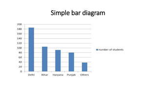
Biostatistics
Dr Md Samiul Islam
BDS(DDCH), MPH(BSMMU), DDS(BSMMU)
Asst. Prof. Of Dental Public Health
Pioneer Dental College & Hospital
Biostatistics
• Statistics- It is a field of study which deals/ concern with the discipline
of collecting, classifying, summarizing and analyzing interpretation
and presentation of data to make scientific interferences.
• Biostatistics- It is the method of collection, organizing, analyzing,
tabulating and interpretation of data related to living organisms and
human beings.
Use of biostatistics
• To evaluate effectiveness of a drug and method of treatment.
• To find an association between disease and risk factor.
• To define normal range /limit to physiological and biological parameters.
• In epidemiological studies the role of risk factor is statistically tested.
• Evaluation of dental health and procedure.
• Use to provide quality control in pharmaceutical industry.
• Data collection
• Data processing
• Data analysis and interpretation
• Drawing of interference
Data
• A set of values recorded on one or more observational units.
• The term data refers to groups of information that represent the
qualitative or quantitative attributes of a variable or set of variable
• Data is the collection of information from the sample or population
for classifying, summarizing and analyzing for making any scientific
interferences.
• Datum is the singular of data.
Types of data
• On the basis of the source
1. Primary data
• Example- data obtained directly from population about their illness.
2. Secondary data
• Example – data collected from hospital records.
3. Tertiary data- in the form of published reports
• On the basis of the nature
1. Quantitative data – example- weight of a person
2. Qualitative data- example- male, female
• Others
• Continuous data- height, weight etc
• Discrete data- no of deaths due to particular disease.
Method of data collection
• Mail questionnaire
• Document review
• Survey
• Observation
• Participatory
• Non-participatory
• Experiment
• In depth review
• Focus group discussion (FGD)
• Case study
Use of data
• To define normal range/ limit
• in designing a healthcare programme or facility.
• To test whether the difference between the two populations,
regarding a particulate attribute is real or just a chance occurrence.
• To study the association between two or more attributes in the same
population.
• To evaluate the effectiveness of an ongoing programme.
• To determine the requirements of a specific population.
• To evaluate the scientific accuracy of a journal article.
Data presentation
• There are two methods of presenting the data
• Tabulation
• Charts and diagrams/ graphical presentation
Tabulation
• Tables are simple device used for the presentation of statistical data.
• The distribution of total data no. of observation among the various
categories is termed as a frequency distribution.
• Tables can be simple or complex depending upon measurement of single
set of items or multiples set of items.
• PRINCIPLES: –
• A table should be numbered
• A title should be given to each table which should be brief and self explanatory.
• Each row and column should be labelled concisely and clearly. The headings of the
columns and rows should be clear, brief and self explanatory
• Tables should be as simple as possible.(2-3 small tables).
• Data should be presented according to size or importance, chronologically or
alphabetically.
• If averages or percentages are to be compared they should be placed as close as
possible.
• Vertical arrangement is better and preferred than horizontal
• Foot notes can be given if necessary
Tabulation
Charts and diagrams/ graphical presentation
• Presenting data in these forms is useful in simplifying the
presentation and enhancing comprehension of the data. Presentation
of data in these forms provides the following
• They simplify the complexity
• Facilitate visual comparison of data
• Arouse the interest of the reader
• Graphs helps a great deal in the analysis of the data
• Provides a more lasting effect on the brain
• Various valuable statistics like median,mode may be easily computed
Charts and diagrams/ graphical presentation
• Disadvantages
• Presentation of graphs is time consuming
• Its facility for comparative analysis is limited
• Measures from the graph will not be accurate
• The conclusions draw from the graphs will not be precise
Charts and diagrams/ graphical presentation
• Diagrams
• Presentation of qualitative, discrete or counted data is through diagrams. The
common diagrams are
• Simple bar diagram
• Multiple bar diagram
• Pie or sector diagram
• Pictogram or picture diagram
• Map diagram or spot diagram
Bar diagram
• A bar diagram is a visual tool that uses bars to compare data among
categories. A bar may run horizontally or vertically
• Consist of two axis
• On a vertical bar graph, the x-axis show data categories and the y-axis
is the scale.
• Bar charts can show big changes of data over time
Simple bar diagram
Multiple bar diagram
Percent/component bar chart
Pie/ sector diagram
Pictogram or picture diagram
Map
/
spot
diagram
Charts and diagrams/ graphical presentation
• Graphs
• Presentation of quantitative, continuous or measured data is through graphs.
The common graphs used are-
• Histogram
• Frequency polygon
• Frequency curve
• Line chart or graphs
• Cumulative frequency diagram
• Scatter or dot diagram
Histogram
Frequency polygon
Frequency curve
Line charts or graphs
Cumulative frequency diagram
Scatter or dot diagram
Symbols
Population Sample
Size N n
Measures Parameter Statistics
Mean µ 𝑥
Standard
deviation
σ s
Proportion P(π) p
Measure of central tendency
• In any frequency distribution, normally data are concentrated around
a value or tends to congregate around a value, this tendency is called
central value or central tendency, and measuring this value is called
measures of central tendency.
Central
tendency
Mean Median Mode
Mean
• The centre of distribution. Also known as arithmetic mean.
• The mean is simply the sum of the values divided by the total number of items
in the set. Or which is abtained by summing up all the observations and
divides the total by the total number of observation.
• Most widely used in public health and medicine
• X= 𝑖=1
𝑛
𝑥𝑖
𝑛
=
𝑥1+ 𝑥2+ ………𝑥𝑛
𝑛
• Example – 10 individuals receiving complete denture treatment are of
following ages-
63, 55, 61, 59, 75, 55, 57, 64, 70, 51
• The total is 610
• To obtain the mean. 610 is divided by 10, which is 61.
Mean
• Advantages
• It is easy to understand and easy to calculate
• It is based upon all the observations and more representative than
median and mode
• It is familiar to common man and rigidly defined
• It is capable of further mathematical treatment. It is possible to compute
mean of means
• It is affected by sampling fluctuations. Hence it is more stable.
• Disadvantages
• Arithmetic mean cannot be obtained if a single observation is missing or
lost
• Arithmetic mean is very much affected by extreme values.
• Sometimes it may look ridiculous. Example- if number of children of 5
mothers are respectively 2, 3, 2, 3, 2
than mean number of children of 5 mother are=
2+3+2+3+2
5
=2.50
Median
• one kind of measure of central tendency.
• The median is determined by sorting the data set from lowest to
highest values and taking the data point in the middle of the
sequence. Or
• Median is the value that divides a distribution into two halves and is a
better indicator of central value, where one or more of the lowest or
the highest observations are wide apart or not so evenly distributed
• It is the middle Value In Ordered Sequence
• If Odd n, Middle Value of Sequence, If even n, Average of 2 Middle
Value.
• Example of odd n-
• number of children in 5 families are 4, 2, 4, 3, 1
• Arrange the observations in ascending and descending order gives 1, 2, 3, 4, 4
• So the median is 3
• Example of even n-
• Patients receiving treatment in the diagnosis department of following ages-
Median for even n
The data on the pulse rate per minute of 10 healthy individuals are 82,
79, 60, 76, 63, 81, 68, 74, 60, 75
n=10
Median
• Advantages
• It is rigidly defined
• It is easy to understand and easy to calculate.
• It is not at all affected by extreme values.
• for uneven distribution, median is the average of choice
• Disadvantages
• In case of even number of observations median cannot be determined
exactly.
• It is not based on all the observations.
• Not determined by mathematical exactness.
• It is not capable of further mathematical treatment
Mode
• Mode is the value which most commonly occurs in the distribution or
occurs most frequently in a series of observations.
• Example- values of pulse rate per minute in a group are
71, 72, 73, 68, 71, 71
• So the mode or the most frequently occurring value is 71
Mode
• Advantages
• Mode is easy to understand and easy to calculate.
• Mode is not at all affected by extreme values.
• Mode can be conveniently located even if the frequency
distribution has class intervals of unequal magnitude
• Disadvantages
• Exact location of Mode is often uncertain and ill defined. So not
used in mathematical statistics
• It is not based upon all the observations.
• It is not capable of further mathematical treatment.
• As compared with mean, mode is affected to a great extent by
fluctuations of sampling.
terminologies
• Percentiles
• Deciles
• Quartiles
• Quintiles
Measure of dispersion
• A quantity that measures the variability among the data, or how the
data one dispersed about the average, known as Measures of
dispersion, scatter, or variations.
• Different measure of dispersion are
• Range
• Mean deviation
• Standard deviation
• Co-efficient of variation
• variance
Range
• Measures the difference between the highest and the lowest item of
the data.
• Range = highest observation – lowest observation
• While easy to calculate and understand, the range can easily be
distorted by extreme values.
• Example- age of complete denture patients
63, 55, 61, 59, 51, 70, 55, 75, 57, 64
• Here highest value is 75 and lowest is 51
• Range is expressed as 51 to 75
Mean deviation
• It is also called Average Deviation
• It is defined as the arithmetic average of the deviation of
the various items of a series computed from measures of
central tendency like mean or median.
variance
• It is the variability of observations calculated by squaring the positive or
negative value of all the observations from the mean and then divided by
the number or observation.
• It is denoted by σ2
•Variance =
{(𝑥− 𝑥1)2+{(𝑥−𝑥2)2+⋯+{(𝑥− 𝑥𝑛)2}
𝑛
• If observation is less than 30,
Variance =
{(𝑥− 𝑥1)2+{(𝑥− 𝑥2)2+⋯+{(𝑥− 𝑥𝑛)2}
𝑛−1
Standard deviation
• Most important & widely used
measure of dispersion
• First used by Karl Pearson in 1893
• Also called root mean square
deviations
• It is defined as the square root of
the arithmetic mean of the
squares of the deviation of the
values taken from the mean
• Denoted by σ (sigma)
Importance of standard deviation
• Standard deviation shows that how data is scattered from the mean
• It summarizes the deviation of a large distribution from its mean in
one figure used as a unit of variation
• It helps to indicate whether variation of difference of an individual
from the mean is by chance
• It helps in finding the suitable size of sample in sampling technique
Co-efficient of variation
• Co-efficient of Variation (CV) Can be used to compare two
or more sets of data measured in different units or same
units but different average size
• Co-efficient of variation(CV) =
𝑆𝐷
𝑚𝑒𝑎𝑛
x 100
Example of measures of central tendency
• Example 1----1, 2, 3, 4, 5
• Mean =
1+2+3+4+5
5
= 3
• median=
𝑛+1
2
=
5+1
2
= 3
• Example 2-----1,2,3,4,5,6
• mean=
1+2+3+4+5+6
6
= 3.5
• median=
𝑥𝑛
2
+𝑥𝑛
2+1
2
=
3+4
2
= 3.5
• Example 3---- 1,1,2,3,3,3,4,4,5,5
• Mean =
𝑓𝑥
𝑓
=
2+2+9+8+10
10
= 3.1
• median=
𝑥𝑛
2
+𝑥𝑛
2+1
2
=
3+3
2
= 3
• Mode= 3 (most frequently
occurring value)
Example of measures of dispersion
• Example – 1,2,3,4,5 where mean is 3
• Range is 1 to 5
• Mean deviation= 𝑖=1
𝑛
𝑥𝑖−𝑥
𝑛
=
1−3 + 2−3 + 3−3 + 4−3 + 5−3
5
=
2+1+0+1+2
5
=
6
5
= 1.2
• Variance σ2 =
(𝑥𝑖−𝑥)2
𝑛
=
(1−3)2+(2−3)2+(3−3)2+(4−3)2+(5−3)2
𝑛
=
4+1+0+1+4
5
= 2
• Standard deviation σ = σ2 =
(𝑥𝑖−𝑥)2
𝑛
= 2 = 1.4142
Normal distribution curve
Properties of normal distribution curve
• The normal distribution curve is bell-shaped.
• It is symmetrical in distribution
• The mean, median, and mode are equal and located at the center of the distribution.
• The curve is continuous.
• The tails never touches the base line or x-axis theoratically
• 68% observtions are found in between +1 and -1 standard deviation
• 95% observtions are found in between +2 and -2 standard deviation
• 99.7% observtions are found in between +3 and -3 standard deviation
• Normal distribution is arithmetically expressed as
• Mean ± 1 SD = 68.27% of the observation
• Mean ± 2 SD = 95.45% of the observation
• Mean ± 3 SD = 99,73% of the observation
Application of normal distribution curve
• Estimate unknown popular parameter
• Test hypothesis
• From the knowledge of µ and σ the area covered under any two
points that is the probability of a random variable lying within a given
range can be worked out.
P value
• P value is defined as the probability of obtaining a result equal to or more extreme than what was
actually observed.
• The p-value was first introduced by Karl Pearson in his Pearson's chi-squared test .
• Ho(Null Hypothesis): Assumes that the two population being compared are not different.
• HA/H1 (Alternative Hypothesis): Assumes that the two groups are different.
• We test the null hypothesis and if there is enough evidence to say that the null hypothesis is
wrong ,we reject the null hypothesis in favour of the alternative hypothesis.
• Rejecting null hypothesis suggests that the alternative hypothesis may be true.
• Type I error –
• False positive conclusion
• stating difference when there is no difference
• Type II Error
• false negative conclusion
• Stating no difference when actually there is i.e. missing a true difference
• Occurs when sample size is too small.
Cut off for p value
• Arbitrary cut-off 0.05 (5% chance of a false +ve conclusion.
• If p<0.05 statistically significant- Reject H0, Accept H1
• If p>0.05 statistically not-significant- Accept H0, Reject H1
• Chi squared test (to study association between two qualitative
variables
• Z test and t test
• quantitative test applied to compare means of two samples or a sample and
the population
• Z test applied when the sample size is large
• T test applied when the sample size is small
• Correlation and regression study the relationship between two or
more continuous variables
Selection of test statistics
Independent
variable
Dependent variable
Discrete Continuous
Discrete Chi-squared test t-test
Z-test
ANOVA
Continuous t-test
Z-test
ANOVA
Correlation
Regression
Thank you

Biostatistics.pptx

  • 1.
    Biostatistics Dr Md SamiulIslam BDS(DDCH), MPH(BSMMU), DDS(BSMMU) Asst. Prof. Of Dental Public Health Pioneer Dental College & Hospital
  • 2.
    Biostatistics • Statistics- Itis a field of study which deals/ concern with the discipline of collecting, classifying, summarizing and analyzing interpretation and presentation of data to make scientific interferences. • Biostatistics- It is the method of collection, organizing, analyzing, tabulating and interpretation of data related to living organisms and human beings.
  • 3.
    Use of biostatistics •To evaluate effectiveness of a drug and method of treatment. • To find an association between disease and risk factor. • To define normal range /limit to physiological and biological parameters. • In epidemiological studies the role of risk factor is statistically tested. • Evaluation of dental health and procedure. • Use to provide quality control in pharmaceutical industry. • Data collection • Data processing • Data analysis and interpretation • Drawing of interference
  • 4.
    Data • A setof values recorded on one or more observational units. • The term data refers to groups of information that represent the qualitative or quantitative attributes of a variable or set of variable • Data is the collection of information from the sample or population for classifying, summarizing and analyzing for making any scientific interferences. • Datum is the singular of data.
  • 5.
    Types of data •On the basis of the source 1. Primary data • Example- data obtained directly from population about their illness. 2. Secondary data • Example – data collected from hospital records. 3. Tertiary data- in the form of published reports • On the basis of the nature 1. Quantitative data – example- weight of a person 2. Qualitative data- example- male, female • Others • Continuous data- height, weight etc • Discrete data- no of deaths due to particular disease.
  • 6.
    Method of datacollection • Mail questionnaire • Document review • Survey • Observation • Participatory • Non-participatory • Experiment • In depth review • Focus group discussion (FGD) • Case study
  • 7.
    Use of data •To define normal range/ limit • in designing a healthcare programme or facility. • To test whether the difference between the two populations, regarding a particulate attribute is real or just a chance occurrence. • To study the association between two or more attributes in the same population. • To evaluate the effectiveness of an ongoing programme. • To determine the requirements of a specific population. • To evaluate the scientific accuracy of a journal article.
  • 8.
    Data presentation • Thereare two methods of presenting the data • Tabulation • Charts and diagrams/ graphical presentation
  • 9.
    Tabulation • Tables aresimple device used for the presentation of statistical data. • The distribution of total data no. of observation among the various categories is termed as a frequency distribution. • Tables can be simple or complex depending upon measurement of single set of items or multiples set of items. • PRINCIPLES: – • A table should be numbered • A title should be given to each table which should be brief and self explanatory. • Each row and column should be labelled concisely and clearly. The headings of the columns and rows should be clear, brief and self explanatory • Tables should be as simple as possible.(2-3 small tables). • Data should be presented according to size or importance, chronologically or alphabetically. • If averages or percentages are to be compared they should be placed as close as possible. • Vertical arrangement is better and preferred than horizontal • Foot notes can be given if necessary
  • 10.
  • 11.
    Charts and diagrams/graphical presentation • Presenting data in these forms is useful in simplifying the presentation and enhancing comprehension of the data. Presentation of data in these forms provides the following • They simplify the complexity • Facilitate visual comparison of data • Arouse the interest of the reader • Graphs helps a great deal in the analysis of the data • Provides a more lasting effect on the brain • Various valuable statistics like median,mode may be easily computed
  • 12.
    Charts and diagrams/graphical presentation • Disadvantages • Presentation of graphs is time consuming • Its facility for comparative analysis is limited • Measures from the graph will not be accurate • The conclusions draw from the graphs will not be precise
  • 13.
    Charts and diagrams/graphical presentation • Diagrams • Presentation of qualitative, discrete or counted data is through diagrams. The common diagrams are • Simple bar diagram • Multiple bar diagram • Pie or sector diagram • Pictogram or picture diagram • Map diagram or spot diagram
  • 14.
    Bar diagram • Abar diagram is a visual tool that uses bars to compare data among categories. A bar may run horizontally or vertically • Consist of two axis • On a vertical bar graph, the x-axis show data categories and the y-axis is the scale. • Bar charts can show big changes of data over time
  • 15.
  • 16.
  • 17.
  • 18.
  • 19.
  • 20.
  • 21.
    Charts and diagrams/graphical presentation • Graphs • Presentation of quantitative, continuous or measured data is through graphs. The common graphs used are- • Histogram • Frequency polygon • Frequency curve • Line chart or graphs • Cumulative frequency diagram • Scatter or dot diagram
  • 22.
  • 23.
  • 24.
  • 25.
  • 26.
  • 27.
  • 28.
    Symbols Population Sample Size Nn Measures Parameter Statistics Mean µ 𝑥 Standard deviation σ s Proportion P(π) p
  • 29.
    Measure of centraltendency • In any frequency distribution, normally data are concentrated around a value or tends to congregate around a value, this tendency is called central value or central tendency, and measuring this value is called measures of central tendency. Central tendency Mean Median Mode
  • 30.
    Mean • The centreof distribution. Also known as arithmetic mean. • The mean is simply the sum of the values divided by the total number of items in the set. Or which is abtained by summing up all the observations and divides the total by the total number of observation. • Most widely used in public health and medicine • X= 𝑖=1 𝑛 𝑥𝑖 𝑛 = 𝑥1+ 𝑥2+ ………𝑥𝑛 𝑛 • Example – 10 individuals receiving complete denture treatment are of following ages- 63, 55, 61, 59, 75, 55, 57, 64, 70, 51 • The total is 610 • To obtain the mean. 610 is divided by 10, which is 61.
  • 32.
    Mean • Advantages • Itis easy to understand and easy to calculate • It is based upon all the observations and more representative than median and mode • It is familiar to common man and rigidly defined • It is capable of further mathematical treatment. It is possible to compute mean of means • It is affected by sampling fluctuations. Hence it is more stable. • Disadvantages • Arithmetic mean cannot be obtained if a single observation is missing or lost • Arithmetic mean is very much affected by extreme values. • Sometimes it may look ridiculous. Example- if number of children of 5 mothers are respectively 2, 3, 2, 3, 2 than mean number of children of 5 mother are= 2+3+2+3+2 5 =2.50
  • 33.
    Median • one kindof measure of central tendency. • The median is determined by sorting the data set from lowest to highest values and taking the data point in the middle of the sequence. Or • Median is the value that divides a distribution into two halves and is a better indicator of central value, where one or more of the lowest or the highest observations are wide apart or not so evenly distributed • It is the middle Value In Ordered Sequence • If Odd n, Middle Value of Sequence, If even n, Average of 2 Middle Value. • Example of odd n- • number of children in 5 families are 4, 2, 4, 3, 1 • Arrange the observations in ascending and descending order gives 1, 2, 3, 4, 4 • So the median is 3 • Example of even n- • Patients receiving treatment in the diagnosis department of following ages-
  • 36.
    Median for evenn The data on the pulse rate per minute of 10 healthy individuals are 82, 79, 60, 76, 63, 81, 68, 74, 60, 75 n=10
  • 37.
    Median • Advantages • Itis rigidly defined • It is easy to understand and easy to calculate. • It is not at all affected by extreme values. • for uneven distribution, median is the average of choice • Disadvantages • In case of even number of observations median cannot be determined exactly. • It is not based on all the observations. • Not determined by mathematical exactness. • It is not capable of further mathematical treatment
  • 38.
    Mode • Mode isthe value which most commonly occurs in the distribution or occurs most frequently in a series of observations. • Example- values of pulse rate per minute in a group are 71, 72, 73, 68, 71, 71 • So the mode or the most frequently occurring value is 71
  • 39.
    Mode • Advantages • Modeis easy to understand and easy to calculate. • Mode is not at all affected by extreme values. • Mode can be conveniently located even if the frequency distribution has class intervals of unequal magnitude • Disadvantages • Exact location of Mode is often uncertain and ill defined. So not used in mathematical statistics • It is not based upon all the observations. • It is not capable of further mathematical treatment. • As compared with mean, mode is affected to a great extent by fluctuations of sampling.
  • 40.
  • 41.
    Measure of dispersion •A quantity that measures the variability among the data, or how the data one dispersed about the average, known as Measures of dispersion, scatter, or variations. • Different measure of dispersion are • Range • Mean deviation • Standard deviation • Co-efficient of variation • variance
  • 42.
    Range • Measures thedifference between the highest and the lowest item of the data. • Range = highest observation – lowest observation • While easy to calculate and understand, the range can easily be distorted by extreme values. • Example- age of complete denture patients 63, 55, 61, 59, 51, 70, 55, 75, 57, 64 • Here highest value is 75 and lowest is 51 • Range is expressed as 51 to 75
  • 43.
    Mean deviation • Itis also called Average Deviation • It is defined as the arithmetic average of the deviation of the various items of a series computed from measures of central tendency like mean or median.
  • 44.
    variance • It isthe variability of observations calculated by squaring the positive or negative value of all the observations from the mean and then divided by the number or observation. • It is denoted by σ2 •Variance = {(𝑥− 𝑥1)2+{(𝑥−𝑥2)2+⋯+{(𝑥− 𝑥𝑛)2} 𝑛 • If observation is less than 30, Variance = {(𝑥− 𝑥1)2+{(𝑥− 𝑥2)2+⋯+{(𝑥− 𝑥𝑛)2} 𝑛−1
  • 45.
    Standard deviation • Mostimportant & widely used measure of dispersion • First used by Karl Pearson in 1893 • Also called root mean square deviations • It is defined as the square root of the arithmetic mean of the squares of the deviation of the values taken from the mean • Denoted by σ (sigma)
  • 46.
    Importance of standarddeviation • Standard deviation shows that how data is scattered from the mean • It summarizes the deviation of a large distribution from its mean in one figure used as a unit of variation • It helps to indicate whether variation of difference of an individual from the mean is by chance • It helps in finding the suitable size of sample in sampling technique
  • 47.
    Co-efficient of variation •Co-efficient of Variation (CV) Can be used to compare two or more sets of data measured in different units or same units but different average size • Co-efficient of variation(CV) = 𝑆𝐷 𝑚𝑒𝑎𝑛 x 100
  • 48.
    Example of measuresof central tendency • Example 1----1, 2, 3, 4, 5 • Mean = 1+2+3+4+5 5 = 3 • median= 𝑛+1 2 = 5+1 2 = 3 • Example 2-----1,2,3,4,5,6 • mean= 1+2+3+4+5+6 6 = 3.5 • median= 𝑥𝑛 2 +𝑥𝑛 2+1 2 = 3+4 2 = 3.5 • Example 3---- 1,1,2,3,3,3,4,4,5,5 • Mean = 𝑓𝑥 𝑓 = 2+2+9+8+10 10 = 3.1 • median= 𝑥𝑛 2 +𝑥𝑛 2+1 2 = 3+3 2 = 3 • Mode= 3 (most frequently occurring value)
  • 50.
    Example of measuresof dispersion • Example – 1,2,3,4,5 where mean is 3 • Range is 1 to 5 • Mean deviation= 𝑖=1 𝑛 𝑥𝑖−𝑥 𝑛 = 1−3 + 2−3 + 3−3 + 4−3 + 5−3 5 = 2+1+0+1+2 5 = 6 5 = 1.2 • Variance σ2 = (𝑥𝑖−𝑥)2 𝑛 = (1−3)2+(2−3)2+(3−3)2+(4−3)2+(5−3)2 𝑛 = 4+1+0+1+4 5 = 2 • Standard deviation σ = σ2 = (𝑥𝑖−𝑥)2 𝑛 = 2 = 1.4142
  • 51.
  • 52.
    Properties of normaldistribution curve • The normal distribution curve is bell-shaped. • It is symmetrical in distribution • The mean, median, and mode are equal and located at the center of the distribution. • The curve is continuous. • The tails never touches the base line or x-axis theoratically • 68% observtions are found in between +1 and -1 standard deviation • 95% observtions are found in between +2 and -2 standard deviation • 99.7% observtions are found in between +3 and -3 standard deviation • Normal distribution is arithmetically expressed as • Mean ± 1 SD = 68.27% of the observation • Mean ± 2 SD = 95.45% of the observation • Mean ± 3 SD = 99,73% of the observation
  • 53.
    Application of normaldistribution curve • Estimate unknown popular parameter • Test hypothesis • From the knowledge of µ and σ the area covered under any two points that is the probability of a random variable lying within a given range can be worked out.
  • 54.
    P value • Pvalue is defined as the probability of obtaining a result equal to or more extreme than what was actually observed. • The p-value was first introduced by Karl Pearson in his Pearson's chi-squared test . • Ho(Null Hypothesis): Assumes that the two population being compared are not different. • HA/H1 (Alternative Hypothesis): Assumes that the two groups are different. • We test the null hypothesis and if there is enough evidence to say that the null hypothesis is wrong ,we reject the null hypothesis in favour of the alternative hypothesis. • Rejecting null hypothesis suggests that the alternative hypothesis may be true. • Type I error – • False positive conclusion • stating difference when there is no difference • Type II Error • false negative conclusion • Stating no difference when actually there is i.e. missing a true difference • Occurs when sample size is too small.
  • 55.
    Cut off forp value • Arbitrary cut-off 0.05 (5% chance of a false +ve conclusion. • If p<0.05 statistically significant- Reject H0, Accept H1 • If p>0.05 statistically not-significant- Accept H0, Reject H1
  • 56.
    • Chi squaredtest (to study association between two qualitative variables • Z test and t test • quantitative test applied to compare means of two samples or a sample and the population • Z test applied when the sample size is large • T test applied when the sample size is small • Correlation and regression study the relationship between two or more continuous variables
  • 57.
    Selection of teststatistics Independent variable Dependent variable Discrete Continuous Discrete Chi-squared test t-test Z-test ANOVA Continuous t-test Z-test ANOVA Correlation Regression
  • 58.