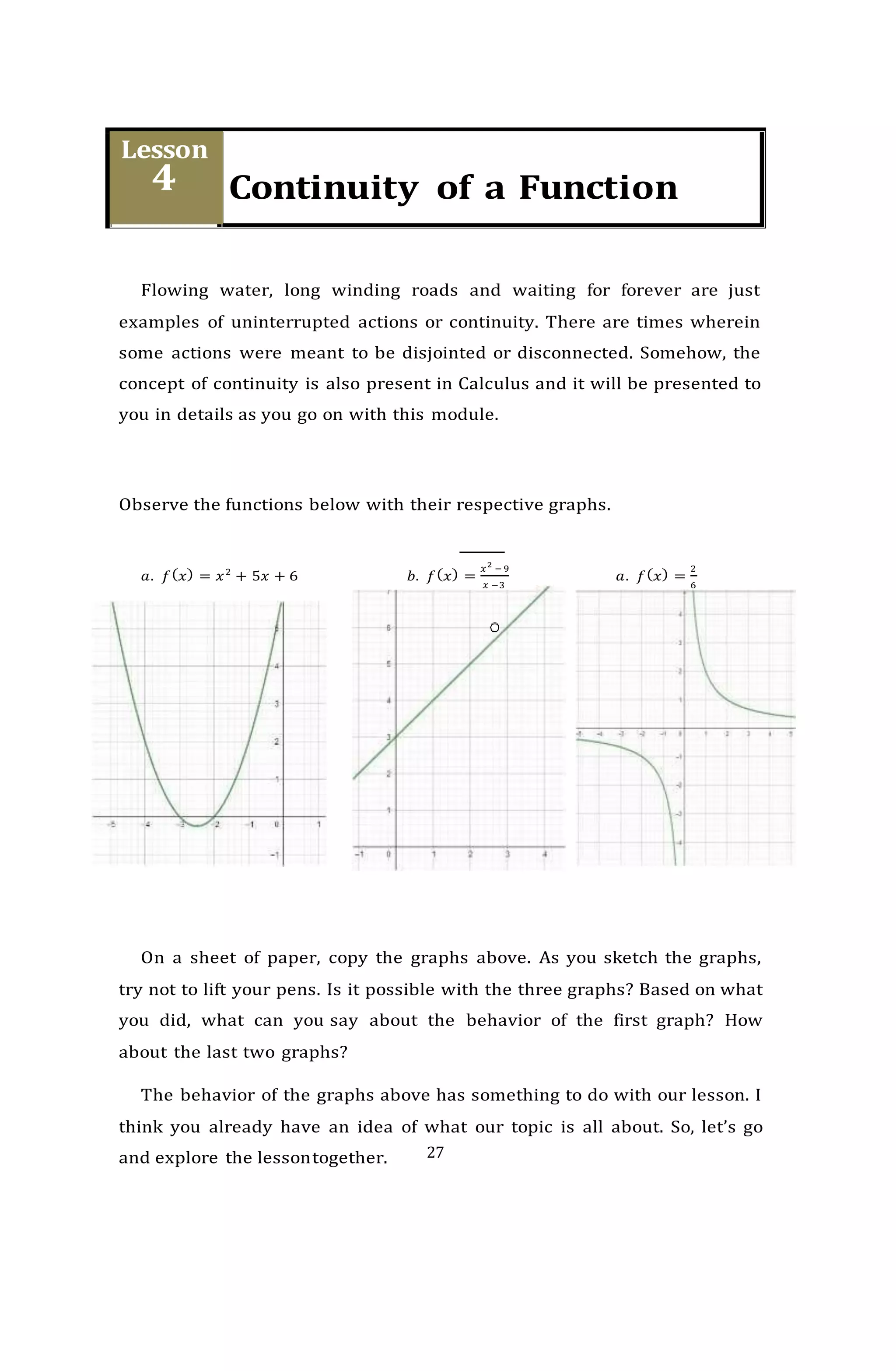
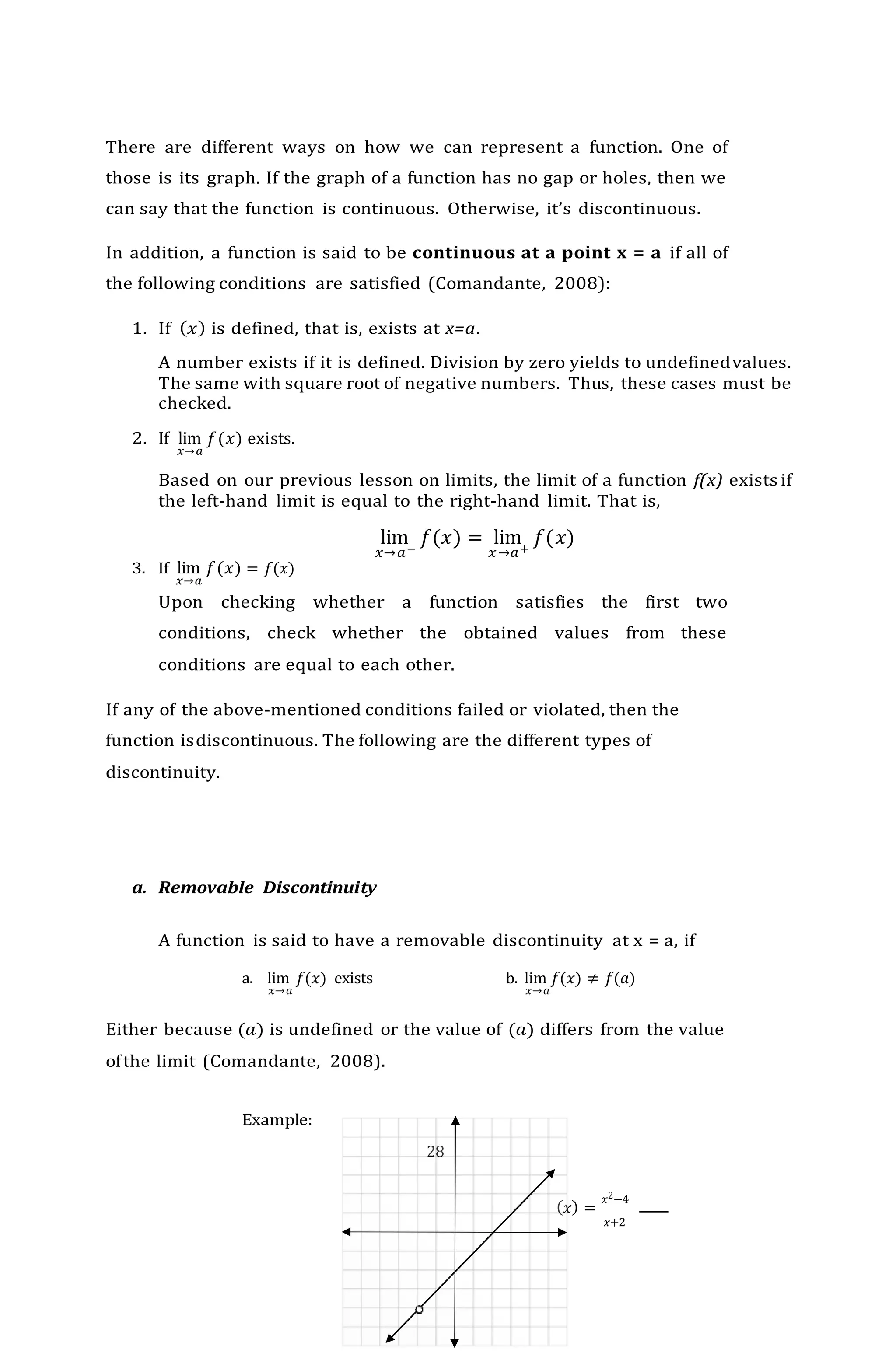
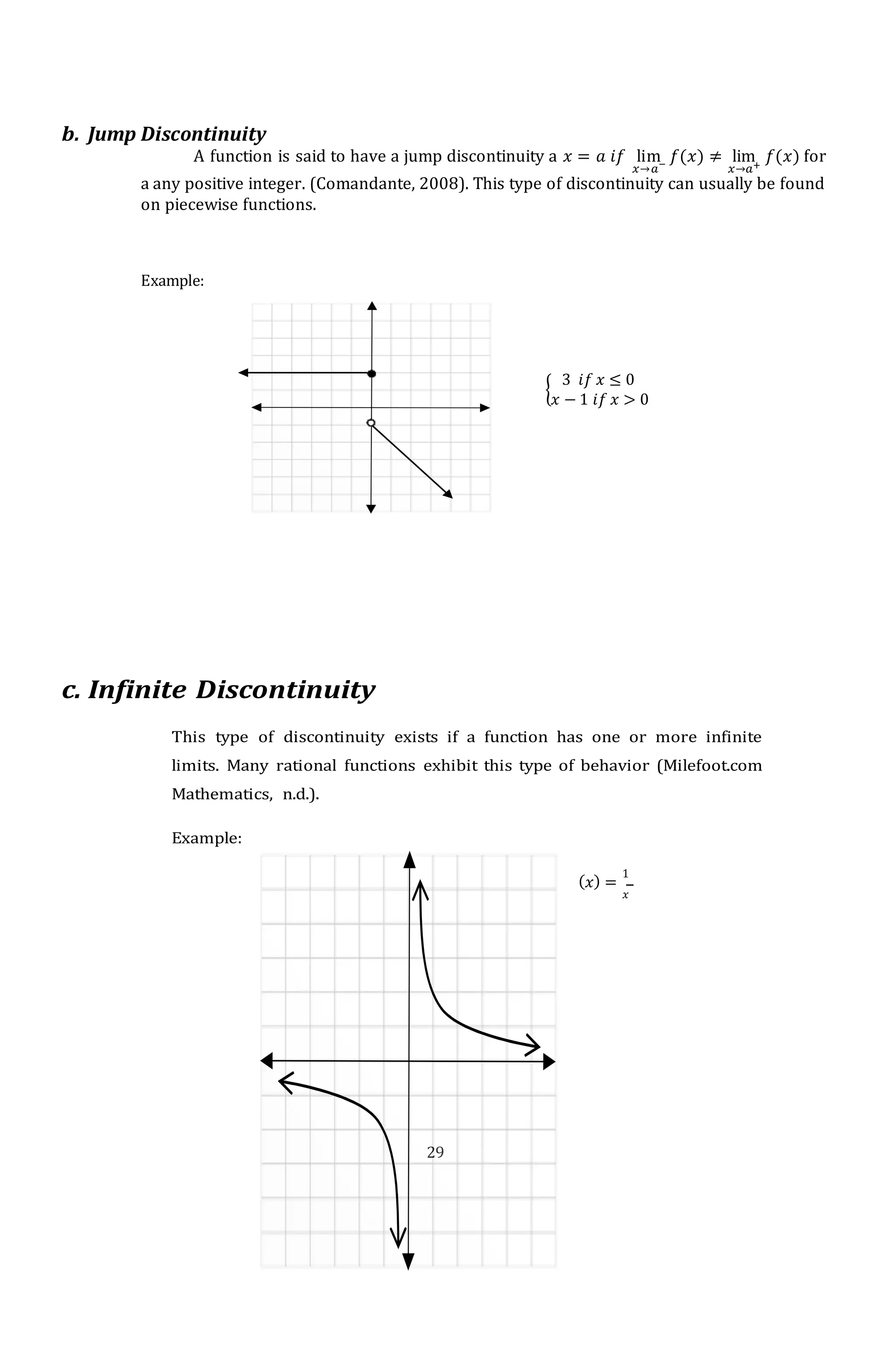
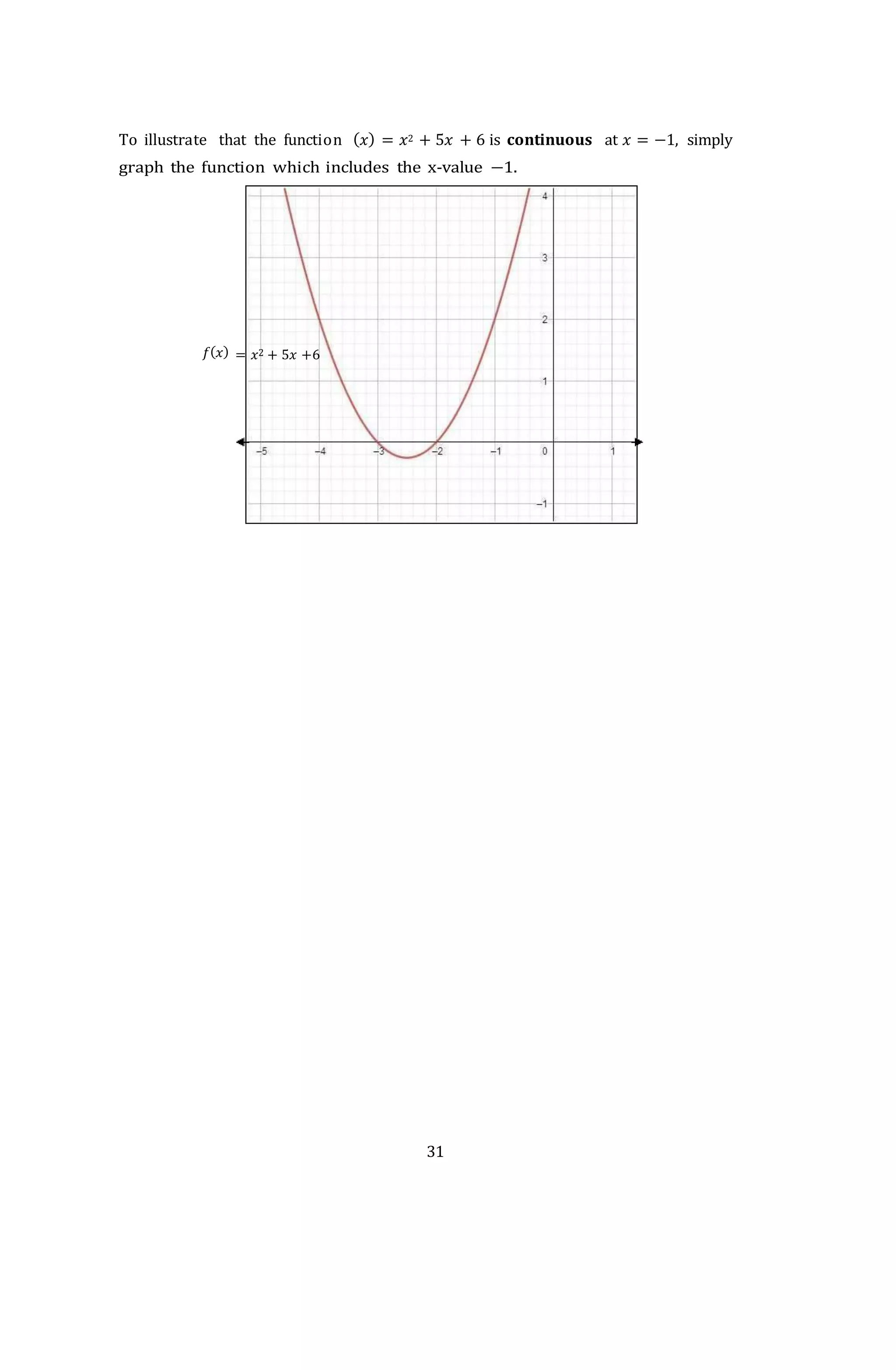
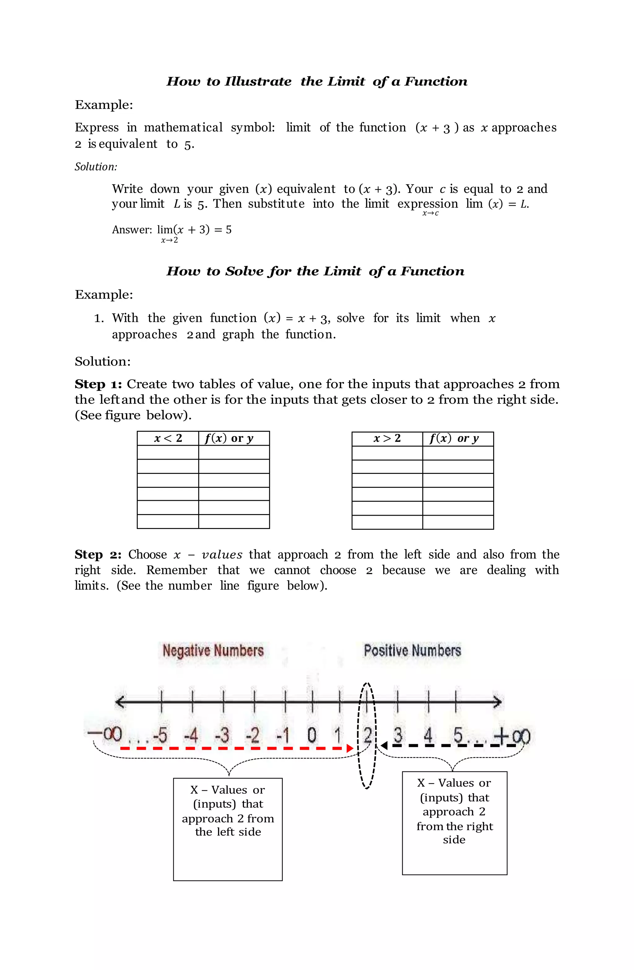
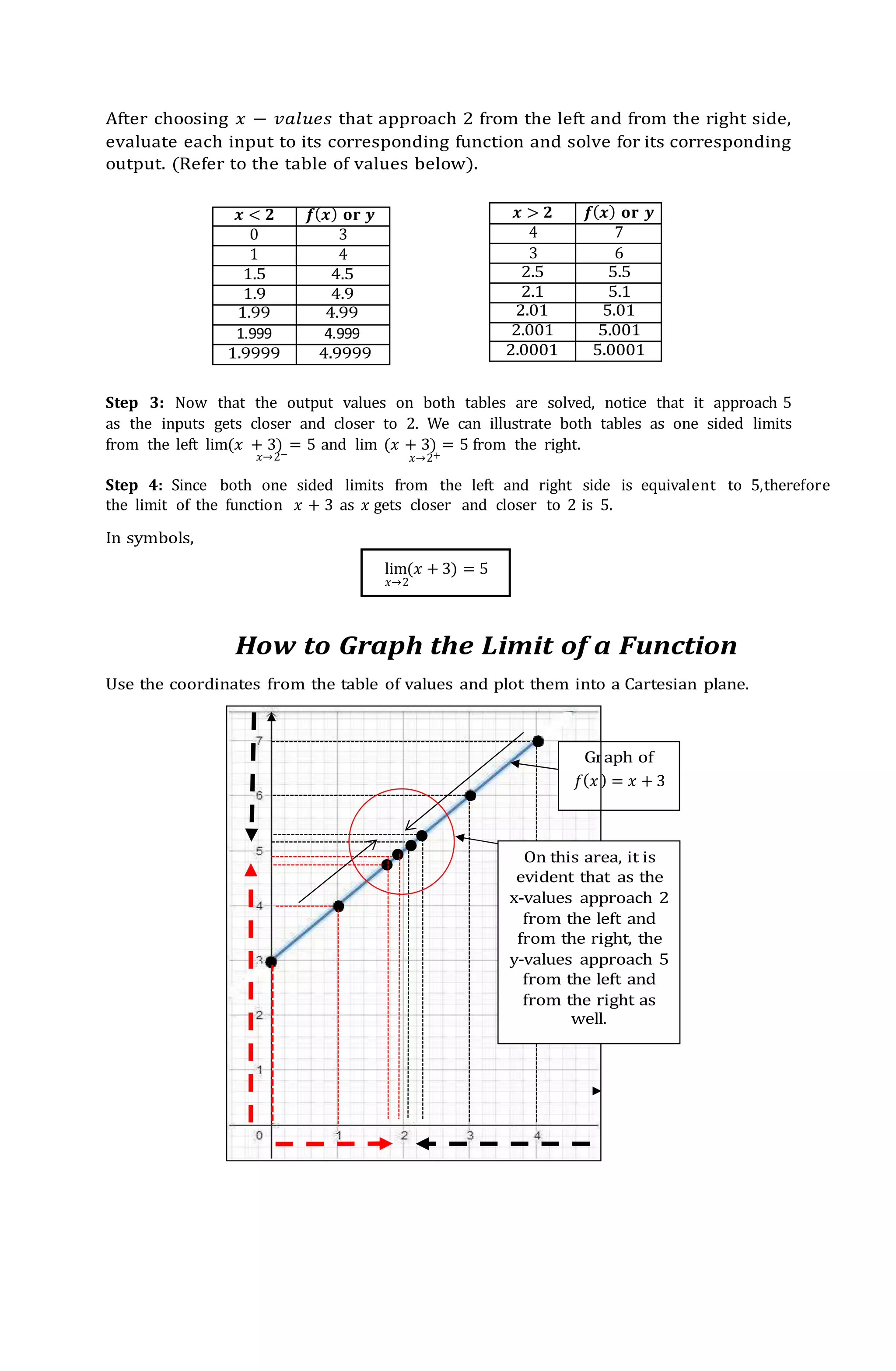
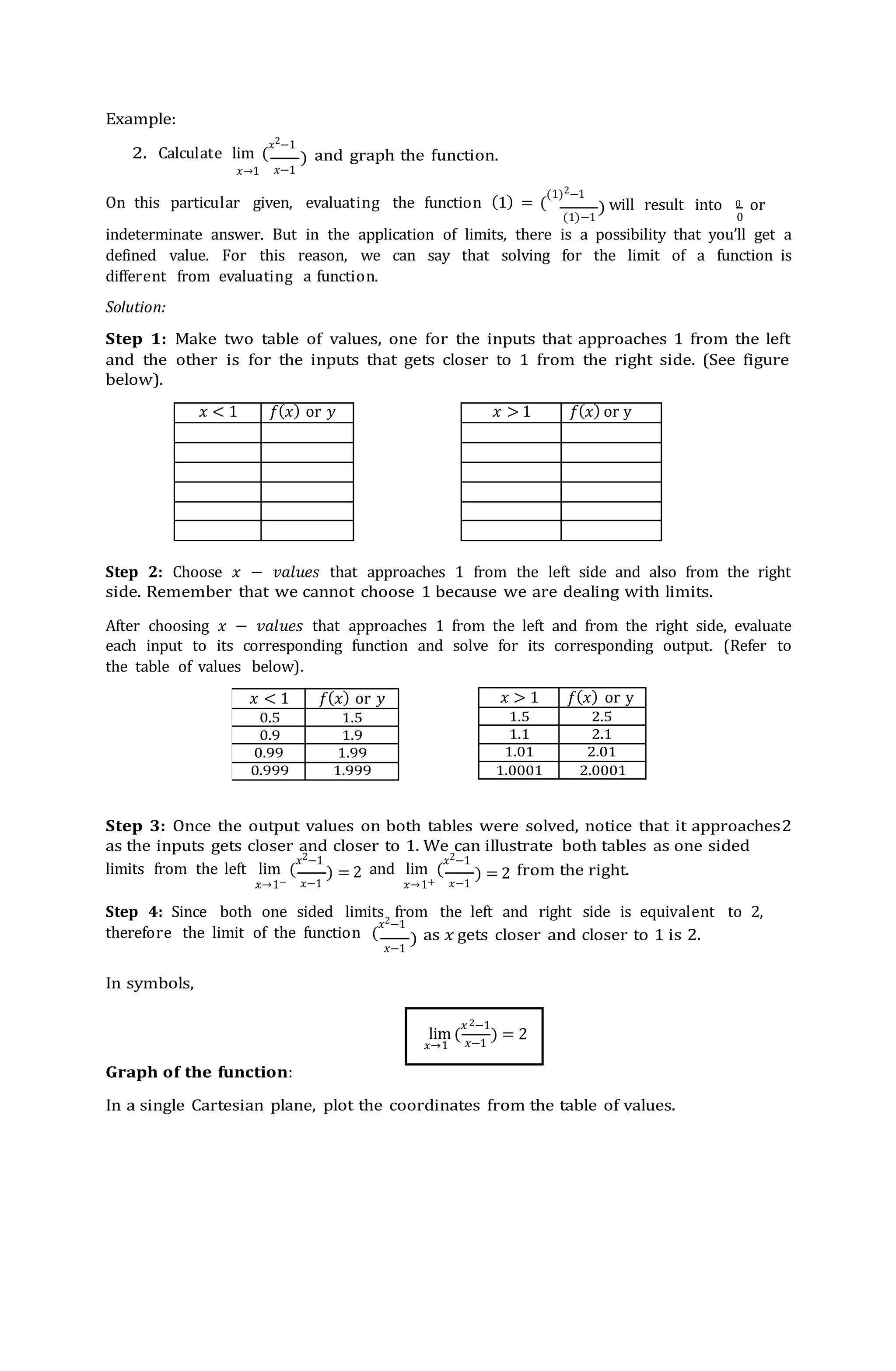
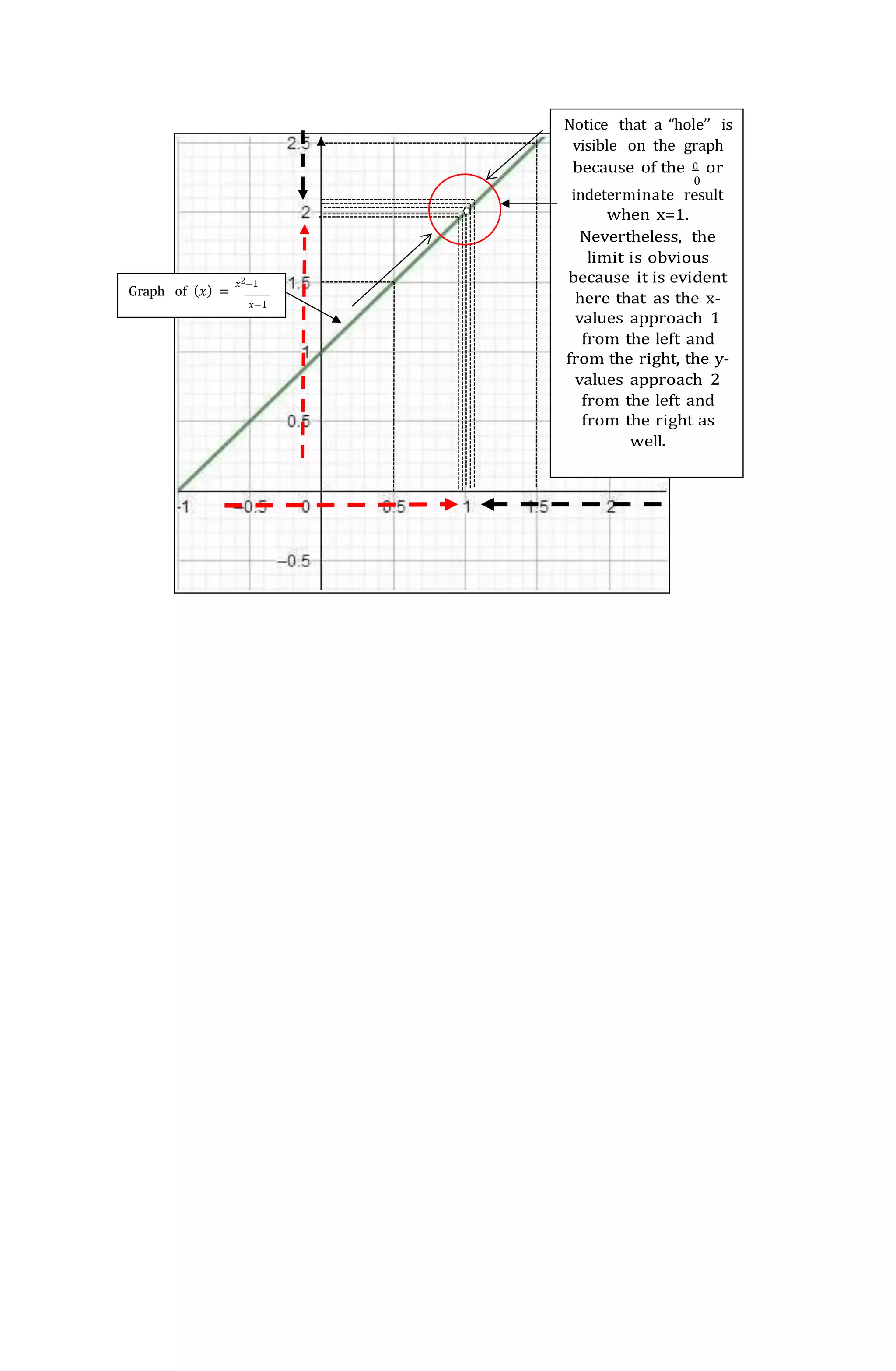
The document discusses limits and how to calculate them. Some key points include: 1. Limits can be calculated by taking the values of a function as it approaches a certain number from the left and right sides. This is done by creating tables of values. 2. Common limit laws can also be used to directly calculate limits, such as the constant multiple law and addition/subtraction laws. 3. Graphing the values from the tables shows whether the limit exists as the input values approach the given number, demonstrating the value the function approaches.

1. From the left side From the right side
Everyone has their own limitation. Knowing your own limit helps you
understand why some things are favorable to you and some are not. In this
branch of Mathematics called Calculus, Limit is one of the important lessons
that you need to understand because it plays a vital role in the application of
differentiation towards a function.
Situation: Have you experienced walking on a street and noticed an image of a
small billboard from afar? Because of the distance, the message on that
billboard is not readable. What action would you take to be able to see clearly
and understand the message on that billboard?
 The limit of a function (𝑥) is the value it approaches as the value of 𝑥
approaches a certain value. “As 𝑥 approaches 𝑎, the limit of (𝑥)
approaches L”. (Mercado, 2016)
This is written in symbols as follows;
𝐥𝐢𝐦 𝒇(𝒙) = 𝑳
𝒙→𝒄
 One sided limit is the value (𝐿) as the 𝒙 value gets closer and closer to
a certain value 𝒄 from one side only (either from the left or from the
right side). In symbols,
𝐥𝐢𝐦 𝒇(𝒙) = 𝑳 𝐥𝐢𝐦 𝒇(𝒙) = 𝑳
𝒙→𝒄− 𝒙→𝒄+
 Always remember that if the limit value from the left side is not equal
to the limit value from the right, then the limit Does Not Exist or DNE.
In symbols, if (𝒙) = 𝑳 ≠ 𝐥𝐢𝐦 𝒇(𝒙) = 𝑳 , then 𝐥𝐢𝐦 𝒇(𝒙) 𝑫𝑵𝑬
𝒙→𝒄− 𝒙→𝒄+ 𝒙→𝒄
 The limit of a function 𝐥𝐢𝐦 𝒇(𝒙) = 𝑳 is not the same as evaluating a function
𝒙→𝒄
(𝒄) because they are different in terms of concept. The limit of a
function gets its value by providing inputs that approaches the particular
number while evaluating a function is more like direct substitution
process.

2. 𝒙 < 𝟐 𝒇(𝒙) or 𝒚 𝒙 > 𝟐 𝒇(𝒙) or y
How to Illustrate the Limit of a Function
Example:
Express in mathematical symbol: limit of the function (𝑥 + 3 ) as 𝑥 approaches
2 is equivalent to 5.
Solution:
Write down your given (𝑥) equivalent to (𝑥 + 3). Your 𝑐 is equal to 2 and
your limit 𝐿 is 5. Then substitute into the limit expression lim (𝑥) = 𝐿.
𝑥→𝑐
Answer: lim(𝑥 + 3) = 5
𝑥→2
How to Solve for the Limit of a Function
Example:
1. With the given function (𝑥) = 𝑥 + 3, solve for its limit when 𝑥
approaches 2and graph the function.
Solution:
Step 1: Create two tables of value, one for the inputs that approaches 2 from
the leftand the other is for the inputs that gets closer to 2 from the right side.
(See figure below).
Step 2: Choose 𝑥 − 𝑣𝑎𝑙𝑢𝑒𝑠 that approach 2 from the left side and also from the
right side. Remember that we cannot choose 2 because we are dealing with
limits. (See the number line figure below).

3. 𝒙 < 𝟐 𝒇(𝒙) or 𝒚
0 3
1 4
1.5 4.5
1.9 4.9
1.99 4.99
1.999 4.999
1.9999 4.9999
𝒙 > 𝟐 𝒇(𝒙) or 𝒚
4 7
3 6
2.5 5.5
2.1 5.1
2.01 5.01
2.001 5.001
2.0001 5.0001
) = 𝑥 + 3
𝑓(𝑥
After choosing 𝑥 − 𝑣𝑎𝑙𝑢𝑒𝑠 that approach 2 from the left and from the right side,
evaluate each input to its corresponding function and solve for its corresponding
output. (Refer to the table of values below).
Step 3: Now that the output values on both tables are solved, notice that it approach 5
as the inputs gets closer and closer to 2. We can illustrate both tables as one sided limits
from the left lim(𝑥 + 3) = 5 and lim (𝑥 + 3) = 5 from the right.
𝑥→2− 𝑥→2+
Step 4: Since both one sided limits from the left and right side is equivalent to 5,therefore
the limit of the function 𝑥 + 3 as 𝑥 gets closer and closer to 2 is 5.
In symbols,
How to Graph the Limit of a Function
Use the coordinates from the table of values and plot them into a Cartesian plane.
lim(𝑥 + 3) = 5
𝑥→2

4. lim (
𝑥 −1
𝑥 < 1 𝑓(𝑥) or 𝑦 𝑥 > 1 𝑓(𝑥) or y
𝑥 < 1 𝑓(𝑥) or 𝑦
0.5 1.5
0.9 1.9
0.99 1.99
0.999 1.999
𝑥 > 1 𝑓(𝑥) or y
1.5 2.5
1.1 2.1
1.01 2.01
1.0001 2.0001
Example:
2. Calculate lim (
𝑥2−1
and graph the function.
𝑥→1 𝑥−1
On this particular given, evaluating the function (1) = (
(1)2−1
(1)−1
will result into 0 or
0
indeterminate answer. But in the application of limits, there is a possibility that you’ll get a
defined value. For this reason, we can say that solving for the limit of a function is
different from evaluating a function.
Solution:
Step 1: Make two table of values, one for the inputs that approaches 1 from the left
and the other is for the inputs that gets closer to 1 from the right side. (See figure
below).
Step 2: Choose 𝑥 − 𝑣𝑎𝑙𝑢𝑒𝑠 that approaches 1 from the left side and also from the right
side. Remember that we cannot choose 1 because we are dealing with limits.
After choosing 𝑥 − 𝑣𝑎𝑙𝑢𝑒𝑠 that approaches 1 from the left and from the right side, evaluate
each input to its corresponding function and solve for its corresponding output. (Refer to
the table of values below).
Step 3: Once the output values on both tables were solved, notice that it approaches2
as the inputs gets closer and closer to 1. We can illustrate both tables as one sided
limits from the left lim (
𝑥2−1
and lim (
𝑥2−1
from the right.
𝑥→1− 𝑥−1 𝑥→1+ 𝑥−1
Step 4: Since both one sided limits from the left and right side is equivalent to 2,
therefore the limit of the function (
𝑥2−1
as 𝑥 gets closer and closer to 1 is 2.
In symbols,
𝑥−1
Graph of the function:
In a single Cartesian plane, plot the coordinates from the table of values.
)
)
) = 2 ) = 2
)

5. Graph of (𝑥) =
𝑥2−1
𝑥−1
Notice that a “hole’’ is
visible on the graph
because of the 0 or
0
indeterminate result
when x=1.
Nevertheless, the
limit is obvious
because it is evident
here that as the x-
values approach 1
from the left and
from the right, the y-
values approach 2
from the left and
from the right as
well.

6. 𝑥 < 2
Input
from
the left
side
𝑓(𝑥) or 𝑦
Output
from the
left side
0 ?
1.5 ?
1.99 ?
1.9999 ?
𝑥 > 2
Input
from the
right
side
𝑓(𝑥) or y
Output
from the
right side
3 ?
2.5 ?
2.01 ?
2.0001 ?
(4 + 𝑥) =
𝑥→2
lim (4 + 𝑥) = _ _ lim (4 + 𝑥) = _
QUIZ
Read and answer the following items. Write your answers on a separate sheet of
paper or use the space in the back of this paper.
1. Evaluate lim(4 + 𝑥).
𝑥→2
One sided limits from the left One sided limits from the right
Graph of the function:
Use the coordinates from the table of values and plot them on the Cartesian plane below.
Limits of Algebraic Expressions
using Tables and Graphs
Lesson
2

7. What are laws and why are they created? For sure there will be lots of
explanation about it, one of which is that, it is a rule that is meant to be
followed for greater good. The Limit lesson has its own laws as well and it
was made because of the advantagesit can provide in solving the limits of
different functions.
Solve for the limit of the given item using the table of values. Write your
solution ona separate sheet of paper. (Use calculator whenever necessary)
Given:
lim
𝑥→3
(
𝑥2
− 𝑥 − 6
𝑥 − 3
)
Table A. (for x values that approaches 3 from the left)
𝑥 2.8 2.9 2.99
𝑦
Table B. (for 𝑥 values that approaches 3 from the right)
𝑥 3.001 3.01 3.1
𝑦
Read and follow the steps in solving the limit of a function using these
different methods. Fill in the blanks to complete the solution of the given.
Copy and answer the table on a separate sheet of paper.
Given:
lim
𝑥→3
(
𝑥2
− 𝑥 − 6
𝑥 − 3
)

8. Steps Solution
1. Observe the given function.
Since it is a rational function,
check whether its numerator
or denominator is factorable.
𝑥2 − 𝑥 − 6 = (𝑥 + _ )(𝑥 − _ )
2. Since the numerator is
factorable, it is evident that
(𝑥 − 3) can be divided.
lim
𝑥→3
|
(𝑥+2)(𝑥−3)
𝑥−3
|=
3. What is left is just (𝑥 + 2), since
it is a polynomial function;
direct substitution is
applicable because it has no
lim(𝑥 + 2)
𝑥→3
domain restrictions.
4. Perform the operation.
[(3) + 2] =
5. Indicate the final answer. lim
𝑥→3
(
𝑥2−𝑥−6
𝑥−3
)=
Limit laws are used as alternative ways in solving the limit of a function
withoutusing table of values and graphs.
Below are the different laws that can be applied in various situations to
solve for thelimit of a function.
A. The limit of a constant is itself. If k is any constant, then,
𝐥𝐢𝐦(𝒌) = 𝒌
𝒙→𝒄
Example:
1. lim(5) = 5
𝑥→𝑐
2. lim(−9) =−9
𝑥→𝑐
B. The limit of 𝑥 as 𝑥 approaches 𝑐 is equal to c. That is,
𝐥𝐢𝐦𝒙 = 𝑪
𝒙→𝒄
Examples:
1. lim (𝑥) = 8
𝑥→8
2. lim (𝑥) = −2
𝑥→−2

9.  For the remaining theorems, we will assume that the limits of f and g
bothexist as x approaches c and that they are L and M, respectively. In other
words,
𝐥𝐢𝐦(𝒙) = 𝑳 and 𝐥𝐢𝐦(𝒙) = 𝑴
𝒙→𝒄 𝒙→𝒄
C. The Constant Multiple Theorem. The limit of a constant 𝑘 times a function is
equal to the product of that constant and its function’s limit.
[𝒌 ∙ 𝒇(𝒙)] = 𝒌 ∙ 𝐥𝐢𝐦 𝒇(𝒙) = 𝒌 ∙ 𝑳
𝒙→𝒄
Examples: If lim 𝑓(𝑥) = 3 , then
𝑥→𝑐
1. lim 5 . (𝑥) = 5 . lim 𝑓(𝑥) = 5 . 3 = 15
𝑥→𝑐 𝑥→𝑐
2. lim (−9). (𝑥) = (−9) . lim 𝑓(𝑥) = (−9) . 3 = −27
𝑥→𝑐 𝑥→𝑐
D. The Addition theorem. The limit of a sum of functions is the sum of the
limits of the individual functions.
𝐥𝐢𝐦 [ 𝒇(𝒙) + 𝒈(𝒙) ] = 𝐥𝐢𝐦 𝒇(𝒙) + 𝐥𝐢𝐦 𝒈(𝒙) = 𝑳 + 𝑴
𝒙→𝒄 𝒙→𝒄 𝒙→𝒄
Examples:
1. If lim 𝑓(𝑥) = 3 and lim 𝑔(𝑥) = −4, then
𝑥→𝑐 𝑥→𝑐
lim ( 𝑓(𝑥) + 𝑔(𝑥)) = lim 𝑓(𝑥) + lim 𝑔(𝑥) = 3 + (−4) = −1
𝑥→𝑐 𝑥→𝑐 𝑥→𝑐
2. If lim (𝑥) = −5 and lim (𝑥) = −2, then
𝑥→𝑐 𝑥→𝑐
lim( 𝑓(𝑥) + 𝑔(𝑥)) = lim 𝑓(𝑥) + lim 𝑔(𝑥) = −5 + (−4) = −9
𝑥→𝑐 𝑥→𝑐 𝑥→𝑐
E. The Subtraction Theorem. The limit of a difference of functions is the
difference of the limits of the individual functions.
𝐥𝐢𝐦 [ 𝒇(𝒙) − 𝒈(𝒙)] = 𝐥𝐢𝐦𝒇(𝒙) − 𝐥𝐢𝐦𝒈(𝒙) = 𝑳 − 𝑴
𝒙→𝒄 𝒙→𝒄 𝒙→𝒄
Examples:
1. If lim 𝑓(𝑥) = 3 and lim 𝑔(𝑥) = −4, then
𝑥→𝑐 𝑥→𝑐
lim ( 𝑓(𝑥) − 𝑔(𝑥)) = lim 𝑓(𝑥) − lim 𝑔(𝑥) = 3 − (−4) = 7
𝑥→𝑐 𝑥→𝑐 𝑥→𝑐
2. If lim (𝑥) = −5 and lim (𝑥) = −2, then
𝑥→𝑐 𝑥→𝑐
lim ( 𝑓(𝑥) − 𝑔(𝑥)) = lim 𝑓(𝑥) − lim 𝑔(𝑥) = −5 − (−4) = −1
𝑥→𝑐 𝑥→𝑐 𝑥→𝑐

10. F. The Multiplication Theorem. The limit of a product of functions is the
product of the limits of the individual functions.
𝐥𝐢𝐦 [ 𝒇(𝒙) ∙ 𝒈(𝒙)] = 𝐥𝐢𝐦 𝒇(𝒙) ∙ 𝐥𝐢𝐦 𝒈(𝒙) = 𝑳 ∙ 𝑴
𝒙→𝒄 𝒙→𝒄 𝒙→𝒄
Examples:
1. If lim 𝑓(𝑥) = 3 and lim 𝑔(𝑥) = −4, then
𝑥→𝑐 𝑥→𝑐
lim( 𝑓(𝑥) . (𝑥)) = lim (𝑥) . lim 𝑔(𝑥) = (3)(−4) = −12
𝑥→𝑐 𝑥→𝑐 𝑥→𝑐
2. If lim (𝑥) = −5 and lim (𝑥) = −2, then
𝑥→𝑐 𝑥→𝑐
lim ( 𝑓(𝑥) . (𝑥)) = lim (𝑥) . lim 𝑔(𝑥) = (−5)(−4) = 20
𝑥→𝑐 𝑥→𝑐 𝑥→𝑐
G. The Division Theorem. The limit of a quotient of functions is the quotient
of the limits of the individual functions, provided that the denominator is not
equal to zero.
𝐥𝐢𝐦
𝒙→𝒄
[
𝒇(𝒙)
𝒈(𝒙)
] =
𝐥𝐢𝐦
𝒙→𝒄
𝒇(𝒙)
𝐥𝐢𝐦
𝒙→𝒄
𝒈(𝒙)
=
𝑳
𝑴
, 𝑴 ≠ 𝟎
Examples:
1. If lim
𝑥→𝑐
𝑓(𝑥) = 3 𝑎𝑛𝑑 lim
𝑥→𝑐
𝑔(𝑥) = −6 ,𝑡ℎ𝑒𝑛
lim
𝑥→𝑐
[
𝑓(𝑥)
𝑔(𝑥)
] =
lim
𝑥→𝑐
𝑓(𝑥)
lim
𝑥→𝑐
𝑔(𝑥)
=
3
−6
= −
1
2
2. If lim
𝑥→𝑐
𝑓(𝑥) = 0 𝑎𝑛𝑑 lim
𝑥→𝑐
𝑔(𝑥) = 7 ,𝑡ℎ𝑒𝑛
lim
𝑥→𝑐
[
𝑓(𝑥)
𝑔(𝑥)
] =
lim
𝑥→𝑐
𝑓(𝑥)
lim
𝑥→𝑐
𝑔(𝑥)
=
0
7
= 0
H. The Power Theorem. The limit of an integer power 𝑝 of a function is just
thatpower of the limit of the function.
𝐥𝐢𝐦
𝒙→𝒄
[𝒇(𝒙)]𝒑
= [𝐥𝐢𝐦𝐟
𝒙→𝒄
(𝒙)]
𝒑
= (𝑳)𝒑
Examples:
1. If lim
𝑥→𝑐
𝑓(𝑥) = 3, 𝑡ℎ𝑒𝑛
lim
𝑥→𝑐
[𝑓(𝑥)]4
= [lim f
𝑥→𝑐
(𝑥)]
4
= (3)4
= 81

11. I. The Radical/Root Theorem. If 𝑛 is a positive integer, the limit of the
𝑛𝑡ℎ rootof a function is just the 𝑛𝑡ℎ root of the limit of the function,
provided that the 𝑛𝑡ℎ root of the limit is a real number.
𝐥𝐢𝐦
𝒙→𝒄
√𝒇(𝒙)
𝒏
= 𝐥𝐢𝐦
𝒙→𝒄
√𝐥𝐢𝐦
𝒙→𝒄
𝒇(𝒙)
𝒏
= √𝑳
𝒏
Examples:
1. If lim
𝑥→𝑐
𝑓(𝑥) = 8 , 𝑡ℎ𝑒𝑛
lim
𝑥→𝑐
√𝑓(𝑥)
3
= lim
𝑥→𝑐
√lim
𝑥→𝑐
𝑓(𝑥)
3
= √8
3
= 2
2. If lim
𝑥→𝑐
𝑓(𝑥) = 64 , 𝑡ℎ𝑒𝑛
lim
𝑥→𝑐
√𝑓(𝑥) = lim
𝑥→𝑐
√lim
𝑥→𝑐
𝑓(𝑥) = √64 = 8
More examples:
1. Find: lim (𝑥2 + 4𝑥 − 3)
𝑥→4
Solution:
Steps Solution
1. Apply Addition Law Theorem. lim(𝑥2) + lim(4𝑥) + lim(−3)
𝑥→4 𝑥→4 𝑥→4
2. Apply Power Theorem on the
first term.
2
[lim 𝑥] + lim(4𝑥) + lim(−3)
𝑥→4 𝑥→4 𝑥→4
3. Apply Multiplication Theorem
on the second term.
2
[lim 𝑥] + 4 [lim 𝑥] + lim(−3)
𝑥→4 𝑥→4 𝑥→4
4. Apply the limit of 𝑥 as
𝑥 approaches 𝑐 is equal to c.
42 + 4(4) + lim(−3)
𝑥→4
5. Apply the limit of a constant is
the constant itself. 42 + 4(4) + (−3)
6. Simplify. 16 + 16 − 3 = 29

12. 1. Solve:
lim
𝑥→1
(
𝑥 + 5
𝑥 + 2
)
Solutions
Steps Solution
1. Apply Division Theorem.
lim(𝑥 + 5)
𝑥→1
lim(𝑥 + 2)
𝑥→1
2. Apply Addition Theorem on the
numerator and denominator.
lim(𝑥) + lim(5)
𝑥→1 𝑥→1
lim(𝑥) + lim(2)
𝑥→1 𝑥→1
3. Apply the limit of 𝑥 as
𝑥 approaches 𝑐 is equal to c.
1 + lim(5)
𝑥→1
1 + lim(2)
𝑥→1
4. Apply the limit of a constant is
the constant itself.
(1) + 5
(1) + 2
5. Simplify. 6
3
= 2

13. QUIZ
Determine the limits of the following items using the limit laws. Write your complete
solutions on the space provided or use the back of this paper if needed.
1. lim
𝑥→5
(𝑥2
− 2𝑥 − 3)
2. lim
𝑥→2
(
𝑥+8
𝑥−7
)
3. lim
𝑥→2
(2𝑥2
− 3𝑥 − 4)

14. Most of the algebraic expressions like “y=x²+6x-2” and “y=x+2” are
composed of letters (or variables) and numbers. They are often used for
the application of limits, but for this lesson non-algebraic expressions
which are called transcendental functions will be utilized.
Recall about the content of module 1, entitled ‘’Limits of Algebraic Function Using
Tables and Graphs’’. In short simple phrases or sentences, explain the process on
how to determine the limit of an algebraic function. Write the answer on a separate
sheet of paper.
Match the graph in column B to its function in column A. Write the letter of the
correct answer on a separate sheet of paper.
Column A Column B
1. 𝑓(𝑥) = 𝑠𝑖𝑛(𝑥) A.
2. 𝑓(𝑥) = 5𝑥 B.
3. 𝑓(𝑥) = log(𝑥) C.

15. For this lesson, we are going to find the limit of a transcendental function
instead of algebraic. Transcendental functions are functions that cannot be
expounded in algebraic form. Some examples of transcendental functions are
exponential [(𝑥) = 10𝑥+1], logarithmic [(𝑥) = log(𝑥 − 2)] and trigonometric
[ℎ(𝑥) = sin(𝑥 + 3)] functions.
The method that will be used in solving the limit of transcendental
function is also table of values and graphs.
Example 1: Exponential function
1. Solve the lim [2(𝑥)] using table of values and sketch its graph.
𝑥→2
SOLUTION:
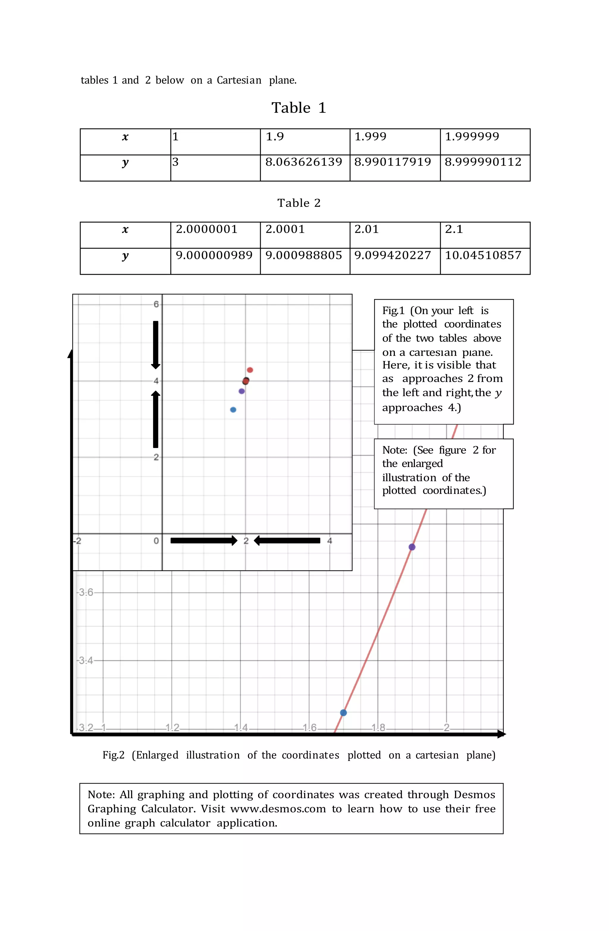
Create two tables for 𝒙 value that approaches 2 from the left and from the right.
Table 1.
𝒙 1.7 1.9 1.99 1.999
𝒚 3.249009585 3.732131966 3.972369982 3.997228372
Table 2.
𝒙 2.001 2.005 2.01 2.1
𝒚 4.00277355 4.013886994 4.0278222 4.28709385
Observation: As the 𝒙 value approaches 2 from the left and right, the 𝒚 value
approaches 4.
After the 𝒚 values on both tables were solved, determine the one-sided limits
from the left and right side.
lim
𝑥→2−
3(𝑥)
= 9 lim
𝑥→2+
3(𝑥)
= 9
Since both one-sided limits from the left and right is equivalent to 9, therefore
thelimit of the function 𝟑𝒙 as 𝒙 gets closer to 2 is 9.
The limit is written as, lim 3𝑥
= 9.
𝑥→2
To illustrate the limit of the function through graph, plot all coordinates from

16. Note: All graphing and plotting of coordinates was created through Desmos
Graphing Calculator. Visit www.desmos.com to learn how to use their free
online graph calculator application.
tables 1 and 2 below on a Cartesian plane.
Table 1
𝒙 1 1.9 1.999 1.999999
𝒚 3 8.063626139 8.990117919 8.999990112
Table 2
𝒙 2.0000001 2.0001 2.01 2.1
𝒚 9.000000989 9.000988805 9.099420227 10.04510857
Fig.2 (Enlarged illustration of the coordinates plotted on a cartesian plane)

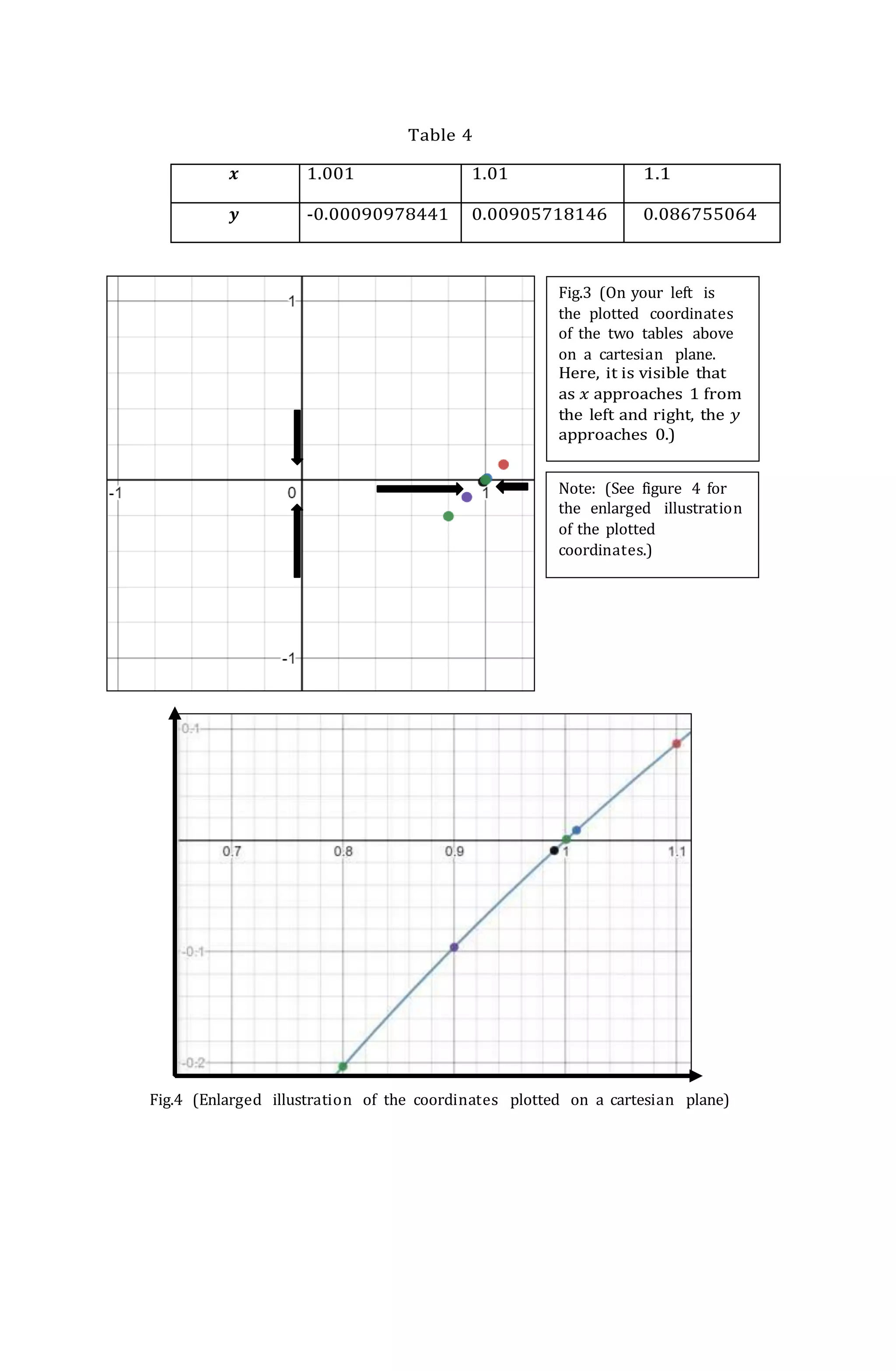
17. Example 2: Logarithmic function
1. Find lim[log3(𝑥)] using table of values and sketch its graph.
𝑥→1
SOLUTION:
Create two tables for 𝒙 value that approaches 1 from the left and from the right.
Table 3.
𝒙 0.8 0.9 0.99
𝒚 -0.203114013 -0.095903274 -0.009148209
Table 4.
𝒙 1.001 1.01 1.1
𝒚 -0.00090978441 0.00905718146 0.086755064
Observation: As the 𝒙 value approaches 1 from the left and right, the 𝒚 value
approaches 0.
After the 𝒚 values on both tables were solved, determine the one-sided limits from
the left and right side.
lim log3(𝑥) = 0 lim log3(𝑥) = 0
𝑥→1− 𝑥→1+
Since both one-sided limits from the left and right is equivalent to 0, therefore
thelimit of the function log3(𝑥) as 𝒙 gets closer to 1 is 0.
The limit is written as lim [log3(𝑥)] = 0 .
𝑥→1
To illustrate the limit of the function through graph, plot all coordinates from
tables3 and 4 on a cartesian plane.
Table 3
𝒙 0.8 0.9 0.99
𝒚 -0.203114013 -0.095903274 -0.009148209

18. Table 4
𝒙 1.001 1.01 1.1
𝒚 -0.00090978441 0.00905718146 0.086755064
Fig.4 (Enlarged illustration of the coordinates plotted on a cartesian plane)
Note: (See figure 4 for
the enlarged illustration
of the plotted
coordinates.)
Fig.3 (On your left is
the plotted coordinates
of the two tables above
on a cartesian plane.
Here, it is visible that
as 𝑥 approaches 1 from
the left and right, the 𝑦
approaches 0.)

19. sin (𝑡)
𝒕
Example 3: Trigonometric function
1. Evaluate lim[ ] using table of values and sketch its graph.
𝑡→0 𝑡
SOLUTION:
Create two tables for 𝒕 value that approaches 0 from the left and from the right.
Onthis example, 𝒕 was used instead of the variable 𝒙.
Table 5.
𝒕 -0.5 -0.2 -0.01
𝒚 0.958851077 0.993346654 0.999983333
Table 6.
𝒕 0.01 0.2 0.5
𝒚 0.999983333 0.993346654 0.958851077

20. Note: (See figure 7 for the
enlarged illustration of
the plotted coordinates.)
Observation: As the 𝑡 value approaches 0 from the left and right, the
𝒚 valueapproaches 1.
After the 𝒚 values on both tables were solved, determine the one-sided limits
from the left and right side.
l
i
m
[
sin(𝑡)
] = 1 lim [
sin(𝑡)
] = 1
𝑡→0− 𝑡 𝑡→0+ 𝑡
Since both one-sided limits from the left and right is equivalent to 1, therefore
thelimit of the function sin(𝑡) as 𝑡 gets closer to 0 is 1.
𝑡
The limit is written as lim [
sin(𝑡)
] = 1 .
𝑡→0 𝑡
To illustrate the limit of the function through graph, plot all coordinates from
tables5 and 6 on a cartesian plane.
Table 5
𝒕 -0.5 -0.2 -0.01
𝒚 0.958851077 0.993346654 0.999983333
Table 6
𝒕 0.01 0.2 0.5
𝒚 0.999983333 0.993346654 0.958851077
Fig.6 (On your left is the
plotted coordinates of the
two tables above on a
cartesian plane. Here, it
is visible that as 𝑡
approaches 0 from the
left and right, the 𝑦
approaches 1.)

21. NOTE: Refer to example 3 for the note about conversion from degree
to radian mode on a scientific calculator
Fig.7 (Enlarged illustration of the coordinates plotted on a cartesian plane)
Example 4: Trigonometric function
1. Sol
ve
1−cos (𝑡)
lim [ ] using table of values and sketch its graph.
𝑡→0 𝑡
SOLUTION:
Create two tables for 𝒕 value that approaches 0 from the left and from the
right.Again, 𝑡 was used instead of the variable 𝒙.
Table 7.
𝒕 -0.5 -0.2 -0.01
𝒚 -0.244834876 -0.09966711 -0.0049999583
Table 8.
𝒕 0.01 0.2 0.5
𝒚 0.0049999583 0.09966711 0.244834876

22. Observation: As the 𝒕 value approaches 0 from the left and right, the 𝒚
valueapproaches 0.
After the 𝒚 values on both tables were solved, determine the one-sided limits from
the left and right side.
l
i
m
[
1−cos(𝑡)
] = 0 lim [
1−cos(𝑡)
] = 0
𝑡→0− 𝑡 𝑡→0+ 𝑡
Since both one-sided limits from the left and right is equivalent to 0, therefore
thelimit of the function 1−cos(𝑡) as 𝑡 gets closer to 0 is 0.
𝑡
The limit is written as lim [
1−cos(𝑡)
] = 0 .
𝑡→0 𝑡
To illustrate the limit of the function through graph, plot all coordinates from
tables7 and 8 on a cartesian plane.
Table 7
𝒕 -0.5 -0.2 -0.01
𝒚 -0.244834876 -0.09966711 -0.0049999583
Table 8
𝒕 0.01 0.2 0.5
𝒚 0.0049999583 0.09966711 0.244834876
Note: (See
figure 9 for the
enlarged
illustration of
the plotted
coordinates.)
Fig.8 (On your
left is the
plotted
coordinates of
the two tables
above on a
cartesian plane.
Here, it is
visible that as 𝑡
approaches 0
from the left
and right, the 𝑦
approaches 0.)

23. Fig.9 (Enlarged illustration of the coordinates plotted on a cartesian plane)
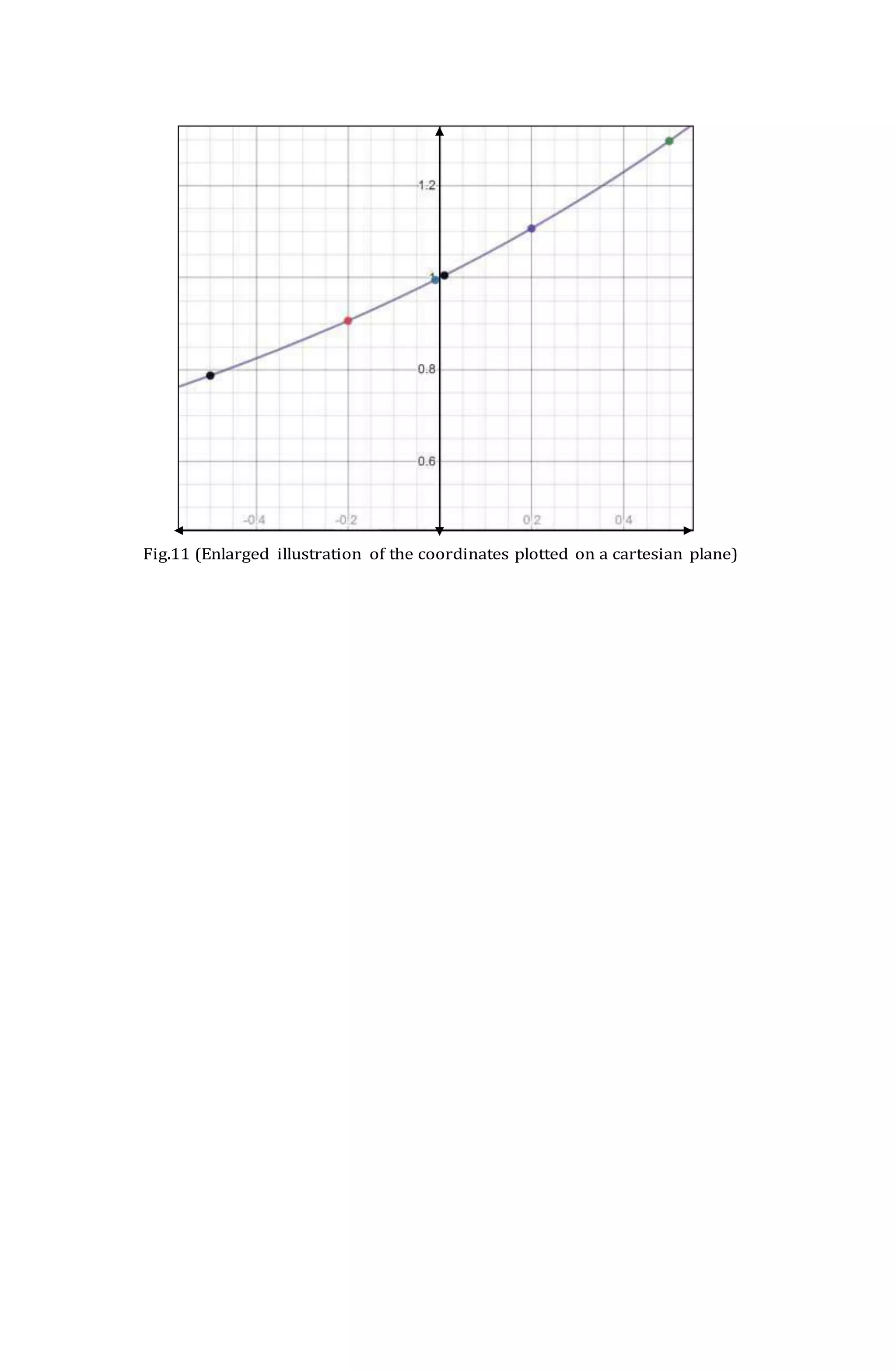
Example 5: Exponential function
5. Determine lim
𝑡→0
[
𝑒𝑡
𝑡
] using table of values and sketch its graph.
SOLUTION:
Create two tables for 𝒕 value that approaches 0 from the left and from the
right.Again, 𝒕 was used instead of the variable 𝒙.
Table 9.
𝒕 -0.5 -0.2 -0.01
𝒚 0.78693868 0.906346234 0.995016624
Table 10.
𝒕 0.01 0.2 0.5
𝒚 1.005016708 1.107013791 1.297442541

24. Note: (See figure 11
for the enlarged
illustration of the
plotted coordinates.)
Observation: As the 𝒕 value approaches 0 from the left and right, the 𝒚
valueapproaches 1.
After the 𝒚 values on both tables were solved, determine the one-sided limits from
the left and right side.
lim
𝑡→0−
[
𝑒𝑡
𝑡
] = 1 lim
𝑡→0+
[
𝑒𝑡
𝑡
] = 1
Since both one-sided limits from the left and right is equivalent to 0, therefore the
limit of the function 𝑒
𝑡-1
𝑡
as 𝒕 get closer to 0 is 1.
The limit is written as lim
𝑡→0
[
𝑒𝑡
𝑡
] = 1
To illustrate the limit of the functionthrough graph, plot all coordinates fromtables 9 and 10
on a cartesian plane.
Table 9
𝒕 -0.5 -0.2 -0.01
𝒚 0.78693868 0.906346234 0.995016624
Table 10
𝒕 0.01 0.2 0.5
𝒚 1.005016708 1.107013791 1.297442541
Fig.10 (On your left is
the plotted
coordinates of the two
tables above on a
cartesian plane. Here,
it is visible that as 𝑡
approaches 0 from
the left and right, the
𝑦 approaches 1.)

25. Fig.11 (Enlarged illustration of the coordinates plotted on a cartesian plane)

26. 26
QUIZ
Answer the following items below. Write your answer on a separate sheet of paper
or use the space at the back of this paper.
1. Evaluate the lim [ln (𝑥)] using table of values.
𝑥→1
Table A (for 𝑥 values that approaches 1 from the left)
𝒙 0.5 0.9 0.999
𝒚
Table B (for 𝑥 values that approaches 1 from the right)
𝒙 1.001 1.01 1.1
𝒚
2. Illustrate the lim [ln (𝑥)] by plotting all coordinates from tables A and B on
a
𝑥→1
cartesian plane.

27. 27
Flowing water, long winding roads and waiting for forever are just
examples of uninterrupted actions or continuity. There are times wherein
some actions were meant to be disjointed or disconnected. Somehow, the
concept of continuity is also present in Calculus and it will be presented to
you in details as you go on with this module.
Observe the functions below with their respective graphs.
𝑎. 𝑓(𝑥) = 𝑥2
+ 5𝑥 + 6 𝑏. 𝑓(𝑥) =
𝑥2
− 9
𝑥 −3
𝑎. 𝑓(𝑥) =
2
6
On a sheet of paper, copy the graphs above. As you sketch the graphs,
try not to lift your pens. Is it possible with the three graphs? Based on what
you did, what can you say about the behavior of the first graph? How
about the last two graphs?
The behavior of the graphs above has something to do with our lesson. I
think you already have an idea of what our topic is all about. So, let’s go
and explore the lessontogether.

28. 28
There are different ways on how we can represent a function. One of
those is its graph. If the graph of a function has no gap or holes, then we
can say that the function is continuous. Otherwise, it’s discontinuous.
In addition, a function is said to be continuous at a point x = a if all of
the following conditions are satisfied (Comandante, 2008):
1. If (𝑥) is defined, that is, exists at x=a.
A number exists if it is defined. Division by zero yields to undefinedvalues.
The same with square root of negative numbers. Thus, these cases must be
checked.
2. If lim
𝑥→𝑎
𝑓(𝑥) exists.
Based on our previous lesson on limits, the limit of a function f(x) exists if
the left-hand limit is equal to the right-hand limit. That is,
lim
𝑥→𝑎−
𝑓(𝑥) = lim
𝑥→𝑎+
𝑓(𝑥)
3. If lim
𝑥→𝑎
𝑓(𝑥) = 𝑓(𝑥)
Upon checking whether a function satisfies the first two
conditions, check whether the obtained values from these
conditions are equal to each other.
If any of the above-mentioned conditions failed or violated, then the
function isdiscontinuous. The following are the different types of
discontinuity.
a. Removable Discontinuity
A function is said to have a removable discontinuity at x = a, if
a. lim 𝑓(𝑥) exists b. lim 𝑓(𝑥) ≠ 𝑓(𝑎)
𝑥→𝑎 𝑥→𝑎
Either because (𝑎) is undefined or the value of (𝑎) differs from the value
ofthe limit (Comandante, 2008).
Example:
(𝑥) =
𝑥2−4
𝑥+2

29. 29
b. Jump Discontinuity
A function is said to have a jump discontinuity a 𝑥 = 𝑎 𝑖𝑓 lim
𝑥→𝑎−
𝑓(𝑥) ≠ lim
𝑥→𝑎+
𝑓(𝑥) for
a any positive integer. (Comandante, 2008). This type of discontinuity can usually be found
on piecewise functions.
Example:
{
3 𝑖𝑓 𝑥 ≤ 0
𝑥 − 1 𝑖𝑓 𝑥 > 0
c. Infinite Discontinuity
This type of discontinuity exists if a function has one or more infinite
limits. Many rational functions exhibit this type of behavior (Milefoot.com
Mathematics, n.d.).
Example:
(𝑥) =
1
𝑥

30. 30
For deeper understanding of the lesson, let us have the following
illustrative examples:
Example1
Identify whether the function (𝑥) = 𝑥2 + 5𝑥 + 6 is continuous at 𝑥 = −1.
Justify youranswer.
Solution:
Check whether the function will satisfy the three conditions for
continuity atthe given point 𝑥 = −1.
a. (𝑥) is defined, that is, exists at x=a.
(𝑥) = 𝑥2 + 5𝑥 + 6, 𝑥 = −1 (Given)
(−1) = (−1)2 + 5(−1) + 6 (Substituted the x-value to the function)
(−1) = 1 − 5 + 6 (Simplified form)
(−1) = 2
Since f(x) exists, then the first condition is satisfied.
b. lim 𝑓(𝑥) exists.
𝑥→𝑎
(𝑥) = 𝑥2 + 5𝑥 + 6 (Given)
lim 𝑓(𝑥) = lim (𝑥2) + lim (5𝑥) + lim 6 (Evaluated the limit)
𝑥→𝑎 𝑥→−1 𝑥→−1 𝑥→−1
lim 𝑓(𝑥) = (−1)2 + 5(−1) + 6 (Simplified form)
𝑥→𝑎
lim 𝑓(𝑥) = 2
𝑥→𝑎
Since lim (𝑥) exists, then the second condition is
satisfied.
𝑥→𝑎
3. lim 𝑓(𝑥) = 𝑓(𝑐)
𝑥→𝑎
Using the obtained values above, let us check if the third condition
willbe satisfied.
lim 𝑓(𝑥) = 𝑓(𝑐) (Third Condition)
𝑥→𝑎
2 = 2 (Obtained values from the solutions above)
Since the two values are equal, then the third condition is satisfied.
Since all of the three conditions were satisfied, then we can say that the function
(𝑥) = 𝑥2 + 5𝑥 + 6 is continuous at 𝑥 = −1.

31. 31
Continuous at x = -1
To illustrate that the function (𝑥) = 𝑥2 + 5𝑥 + 6 is continuous at 𝑥 = −1, simply
graph the function which includes the x-value −1.
𝑓(𝑥) = 𝑥2 + 5𝑥 +6
6666

32. 32
QUIZ
Express what you have learned in this lesson by answering the questions below.
Write your answers on a separate sheet of paper or just use the space provided.
1. How to determine whether the function is continuous or not at a certain point?
2. How to determine whether the function is continuous or not on a closed interval?
3. How to illustrate the continuity or discontinuity of a function?