This document is the report for a master's thesis presented by Ignasi Cifre Font and Àlex Garcia Manzanera to obtain a degree in Energy Engineering. The thesis examines the acceleration-based control of offshore fixed wind turbines through simulation and parameter tuning. It includes 7 chapters that describe the objectives, control systems, FAST simulation software, Simulink models developed, simulation results and parameter tuning analyses. The goal is to develop and evaluate an acceleration-based control system and tune its parameters to improve the operation of an offshore fixed wind turbine model compared to a baseline control system.


![List of Figures
1.1 Global annual installed wind capacity 2000-2015. Source: GWEC [Sawyer and
Reve (2016)]. . . . . . . . . . . . . . . . . . . . . . . . . . . . . . . . . . . . . . . . 16
1.2 Global cumulative installed wind capacity 2000-2015. Source: GWEC [Sawyer
and Reve (2016)]. . . . . . . . . . . . . . . . . . . . . . . . . . . . . . . . . . . . . 17
1.3 Global and annual offshore wind capacity. Source: GWEC [Sawyer and Reve
(2016)]. . . . . . . . . . . . . . . . . . . . . . . . . . . . . . . . . . . . . . . . . . . 18
1.4 Types of offshore wind turbines foundations. Source: [Bailey et al. (2014)]. . . . . 19
1.5 Wind turbine elements. Source: U.S. Department of Energy [Office of Energy
and Renewable Energy (2016)]. . . . . . . . . . . . . . . . . . . . . . . . . . . . . . 20
1.6 Wind turbine control block diagram. Source: American Control Conference [Pao
L.Y. and K.E. Johnson (2009)]. . . . . . . . . . . . . . . . . . . . . . . . . . . . . . . 21
2.1 Sensors distribution in the jacket structure (left) and in the nacelle (right). Source:
[Jonkman et al. (2012)]. . . . . . . . . . . . . . . . . . . . . . . . . . . . . . . . . . 27
2.2 Gain factor graphic depending on the blade pitch angle. Source: [Jonkman et al.
(2009)]. . . . . . . . . . . . . . . . . . . . . . . . . . . . . . . . . . . . . . . . . . . 32
3.1 FAST architecture including the driver, input files and output files. Source: [Jonkman
and Jonkman (2016)]. . . . . . . . . . . . . . . . . . . . . . . . . . . . . . . . . . . 37
3.2 FAST distribution modules for fixed-bottom systems. Source: [Jonkman and Jonkman
(2016)]. . . . . . . . . . . . . . . . . . . . . . . . . . . . . . . . . . . . . . . . . . . 39
4.1 Block S_Function. It is the beginning of the process of FAST-Simulink interface. . 42
4.2 Block S-Function once the inputs and outputs are added to the initial block. . . . 43
4.3 Simulink model used to implement the baseline control system. Source: [Jonkman
et al. (2009)]. . . . . . . . . . . . . . . . . . . . . . . . . . . . . . . . . . . . . . . . 46
4.4 Sub-model containing the torque and power controller. Source: [Jonkman et al.
(2009)]. . . . . . . . . . . . . . . . . . . . . . . . . . . . . . . . . . . . . . . . . . . 47
4.5 Sub-model containing the blade pitch angle controller. Source: [Jonkman et al.
(2009)]. . . . . . . . . . . . . . . . . . . . . . . . . . . . . . . . . . . . . . . . . . . 48
4.6 Simulink model implementation of acceleration-based control system. Source:
[Tutivén et al. (2015)]. . . . . . . . . . . . . . . . . . . . . . . . . . . . . . . . . . . 49
4.7 Torque and power controller sub-model. Source: [Tutivén et al. (2015)]. . . . . . . 50
4.8 Blade pitch angle controller sub-model. Source: [Tutivén et al. (2015)]. . . . . . . 51
v](https://image.slidesharecdn.com/d5dea01b-1c58-4cb9-b6c8-8c7a99c48f71-161121112012/85/BACHELOR_THESIS_ACCELERATIOM-BASED_CONTROL_OF_OFFSHORE_WT-7-320.jpg)
![LIST OF FIGURES Ignasi Cifre and Àlex Garcia
4.9 Generator torque and speed while start process of the turbine. Source: [Jonkman
et al. (2009)]. . . . . . . . . . . . . . . . . . . . . . . . . . . . . . . . . . . . . . . . 52
4.10 Wind velocity [m/s]. . . . . . . . . . . . . . . . . . . . . . . . . . . . . . . . . . . 53
4.11 Wave elevation [m]. . . . . . . . . . . . . . . . . . . . . . . . . . . . . . . . . . . . 54
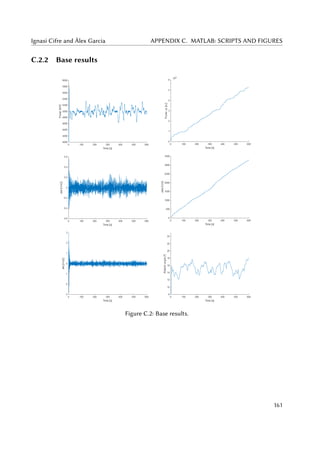
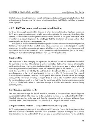
5.1 Power output (left) and power index Jp (right) for the base simulation. . . . . . . 60
5.2 Torque signal τr (left) and generator speed ωg (right) for the base simulation. . . . 60
5.3 Side-to-side acceleration (left) and Jass index (right) for the base simulation. . . . 61
5.4 Fore-aft acceleration (left) and blade pitch angle (right) for the base simulation. . 61
5.5 Power zoom (left) and Jp (right) for different α1 in the first set of simulations. . . 64
5.6 Power output (left) and Jp (right) for different α2 in the first set of simulations. . 64
5.7 ass (left) and Jass (right) for different α2 in the first set of simulations. . . . . . . 65
5.8 Jp (left) and Jass (right) for different α3 in the first set of simulations. . . . . . . . 66
5.9 ass (left) and Jass (right) for different α4 in the first set of simulations. . . . . . . 66
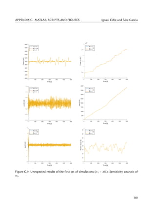
5.10 Power output (left) and its Jp index (right) for α3 with original vs. unexpected
values of α2 . . . . . . . . . . . . . . . . . . . . . . . . . . . . . . . . . . . . . . . 69
5.11 Power output Pe (left) and zoomed in power output Pe (right) for α1 = 20 instead
of the original value. . . . . . . . . . . . . . . . . . . . . . . . . . . . . . . . . . . 71
5.12 Jp (left) and ass (right) for α1 = 20 instead of the original value. . . . . . . . . . . 72
5.13 Real generator torque τr (left) and zoomed in torque (right) for base results and
for α1 = 20. . . . . . . . . . . . . . . . . . . . . . . . . . . . . . . . . . . . . . . . 72
5.14 Pe (left) and zoomed in Pe (right) for α2 = 1000 instead of the original value. . . 73
5.15 Jp (left) and ass (right) for α2 = 1000 instead of the original value. . . . . . . . . 73
5.16 Jp (left) and Jass (right) for α3 = 20 instead of the original value. . . . . . . . . . 74
5.17 Real torque generator τr and reference torque τc for α3 = 20 instead of the
original value. . . . . . . . . . . . . . . . . . . . . . . . . . . . . . . . . . . . . . . 74
5.18 ass (left) and Jass (right) for α4 = 50 instead of the original value. . . . . . . . . . 75
5.19 Blade pitch angle (left) and zoomed in blade pitch angle (right) for α4 = 50
instead of the original value. . . . . . . . . . . . . . . . . . . . . . . . . . . . . . . 76
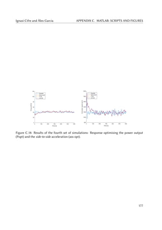
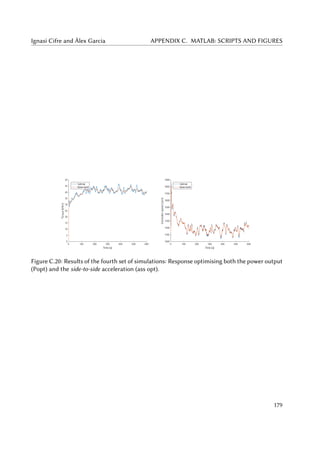
5.20 Pe (left) and zoomed in Pe (right) for various α2. . . . . . . . . . . . . . . . . . . . 77
5.21 Jp (left) and real generator torque τr for various α2. . . . . . . . . . . . . . . . . . 78
5.22 ass (left) and Jass (right) for various α2. . . . . . . . . . . . . . . . . . . . . . . . . 79
5.23 afa (left) and blade pitch angle (right) for various α2. . . . . . . . . . . . . . . . . 80
5.24 Power index Jp for four different combinations. . . . . . . . . . . . . . . . . . . . 82
5.25 Pe (left) and zoomed in Pe (right) for four different combinations. . . . . . . . . . 83
5.26 Realt torque τr (left) and zoomed in real torque (right) for four different combi-
nations. . . . . . . . . . . . . . . . . . . . . . . . . . . . . . . . . . . . . . . . . . . 83
5.27 ass (left) and Jass (right) for four different combinations. . . . . . . . . . . . . . . 84
5.28 afa (left) and blade pitch angle (right) for four different combinations. . . . . . . 85
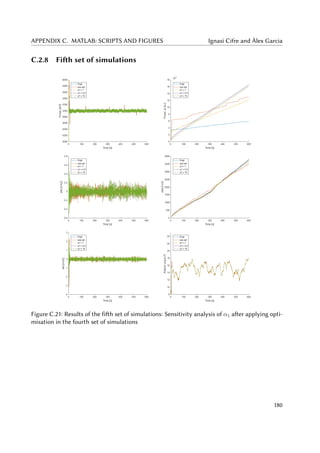
5.29 Pe (left) and zoomed in Pe (right) for the fifth set of simulations. . . . . . . . . . . 87
5.30 Jp for the fifth set of simulations. . . . . . . . . . . . . . . . . . . . . . . . . . . . 88
5.31 ass (left) Jass (right) for the fifth set of simulations. . . . . . . . . . . . . . . . . . 88
vi](https://image.slidesharecdn.com/d5dea01b-1c58-4cb9-b6c8-8c7a99c48f71-161121112012/85/BACHELOR_THESIS_ACCELERATIOM-BASED_CONTROL_OF_OFFSHORE_WT-8-320.jpg)


![List of Tables
1.1 Main properties of the NREL 5 MW wind turbine. Source: [Jonkman et al. (2009)]. 22
3.1 Some tests distributed with FAST v8 using NREL 5 MW turbine. Source: [Jonkman
and Jonkman (2016)]. . . . . . . . . . . . . . . . . . . . . . . . . . . . . . . . . . . 36
5.1 Values for each α of the base simulation. . . . . . . . . . . . . . . . . . . . . . . . 59
5.2 Indices results for base and baseline simulations. . . . . . . . . . . . . . . . . . . 62
5.3 Power and ass results for base and baseline simulations. . . . . . . . . . . . . . . 62
5.4 Alpha values for the first set of simulations. . . . . . . . . . . . . . . . . . . . . . 63
5.5 Alpha values for the unexpected set of simulations. . . . . . . . . . . . . . . . . . 68
5.6 Alpha values for the second set of simulations. . . . . . . . . . . . . . . . . . . . . 70
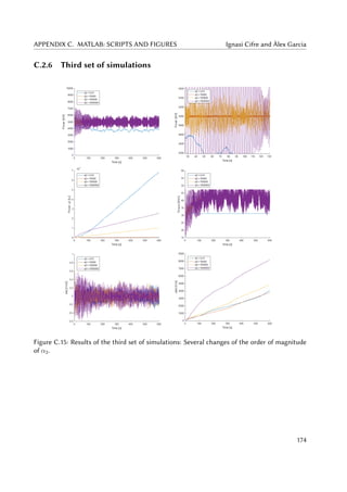
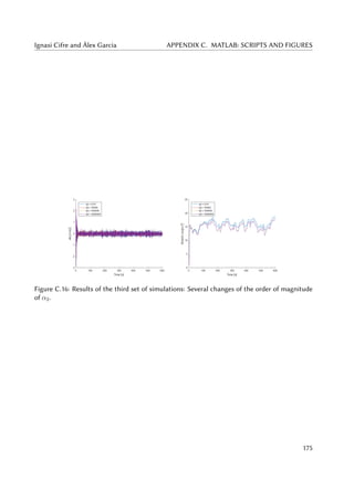
5.7 Alpha values for the third set of simulations. . . . . . . . . . . . . . . . . . . . . . 77
5.8 Power results for different values of α2 in the third set of simulations. . . . . . . . 78
5.9 ass results for different values of α2 in the third set of simulations. . . . . . . . . 79
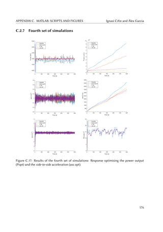
5.10 Alpha values for the fourth set of simulations. . . . . . . . . . . . . . . . . . . . . 81
5.11 Power index for each combination of α2 and α4. . . . . . . . . . . . . . . . . . . . 84
5.12 Jass index for each combination of α2 and α4 [in kJ]. . . . . . . . . . . . . . . . . 84
5.13 Alpha values for the unexpected set of fourth set of simulations. . . . . . . . . . . 86
5.14 Alpha values for the fifth set of simulations. . . . . . . . . . . . . . . . . . . . . . 87
6.1 Optimal range for each of the α gains. . . . . . . . . . . . . . . . . . . . . . . . . 93
6.2 Jp reduction in percentage, Jp of each combination of α2 and α4 over the base
result. . . . . . . . . . . . . . . . . . . . . . . . . . . . . . . . . . . . . . . . . . . . 93
6.3 Jass increment in percentage of each combination of α2 and α4 over the base
result. . . . . . . . . . . . . . . . . . . . . . . . . . . . . . . . . . . . . . . . . . . 94
6.4 Jass reduction in percentage, Jass , of each combination of α2 and α4 over the
baseline result. . . . . . . . . . . . . . . . . . . . . . . . . . . . . . . . . . . . . . . 94
6.5 I1 for the different combinations of α2 and α4. . . . . . . . . . . . . . . . . . . . . 96
6.6 I2 with q = 0.7 for the different combinations of α2 and α4. . . . . . . . . . . . . 96
6.7 Summary of results for the best combinations. . . . . . . . . . . . . . . . . . . . . 97
6.8 Results of the optimal vs base results. . . . . . . . . . . . . . . . . . . . . . . . . . 101
6.9 Differences in kW between optimal, baseline and base combinations in specific
worst moments of the power stability. . . . . . . . . . . . . . . . . . . . . . . . . . 104
ix](https://image.slidesharecdn.com/d5dea01b-1c58-4cb9-b6c8-8c7a99c48f71-161121112012/85/BACHELOR_THESIS_ACCELERATIOM-BASED_CONTROL_OF_OFFSHORE_WT-11-320.jpg)


![Chapter 1
Introduction
Nowadays, first world societies are provided by an energy model based on fuel fossils combus-
tion and uranium fission. This model has enabled the huge development that countries and
communities have experienced during the 20th
century. However, this model is not sustainable
nor environmentally friendly, and the needing of a change is imposed. Moreover, the imminent
exhaustion of fossil fuels imply that the new methodology or basis has to be developed with
no more delay. Consequently, in the following years fossil fuels will be replaced by renewable
sources.
Renewable sources are those sources that are considered inexhaustible for human uses. The
renewable flows integrate many energy forms: solar, wind, hydraulic, geothermal, etc. Generally,
the process of transforming the energy provided by those sources into electrical energy does not
imply the emission of CO2 nor any kind of damaging pollutants or greenhouse effect gases. As
a consequence, it seems obvious that a model based on the use of renewable sources could be
more robust and sustainable than the one we have nowadays, and it has the potential to put an
end to many problems that our world is facing in the 21st
century in terms of energy. Amongst
these problems, one can consider both the limitations and difficulties of a part of the society
to affording energy access and the planet and environment accumulated damage during last
decades.
1.1 Wind energy situation
Within the renewable technologies, wind energy has become really important thanks to the
strengths that it has. It has the ability to produce big amounts of energy at a country-scale, so
it is a technology that states can seriously consider when thinking about energy development
planning of the future. Moreover, it can be produced offshore, where the wind flows are more
constant and with higher velocities.
Consulting the data collection of the Global Wind Energy Council (GWEC) [Sawyer and Reve
(2016)], the upward trend in both installed wind energy power per year and cumulative installed
wind power can be confirmed.
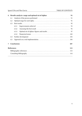
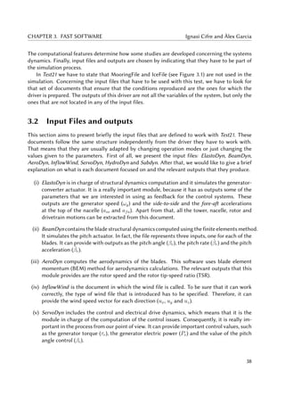
Figure 1.1 shows that since the beginning of the century there has been a constant increase in
15](https://image.slidesharecdn.com/d5dea01b-1c58-4cb9-b6c8-8c7a99c48f71-161121112012/85/BACHELOR_THESIS_ACCELERATIOM-BASED_CONTROL_OF_OFFSHORE_WT-27-320.jpg)
![CHAPTER 1. INTRODUCTION Ignasi Cifre and Àlex Garcia
Figure 1.1: Global annual installed wind capacity 2000-2015. Source: GWEC [Sawyer and Reve
(2016)].
the amount of wind capacity installed every year (there is only one isolated regression in 2013).
Last year, there was a total power installation of around 63000 MW, whereas in the year 2000
the amount of power installed was 3760 MW. This means that the global wind capacity has been
increasing during the last 15 years. Moreover, this growth is not constant, but it increases every
year.
This first graphic shows what was exposed at the beginning, that is, the big change that has
experienced the importance of wind energy in the last few years. At the end of the last century
and the early 2000s, the rate of development of this technology showed that it was an emergent
science. By 2015, the rate of installation of wind energy plants is suitable to determine that wind
is the future of the energy system worldwide.
With regard to the cumulated wind capacity, it is still far from being a crucial energy source,
but thanks to the last fifteen years of development, it is now really important in some areas of
the world, like northern countries of Europe. In Figure 1.2 one can see that the global wind power
during last fifteen years has increased a 25000%. That may seem a big achievement, and in fact
it is, but is still far from what is needed if renewable systems want to replace fossil fuels in the
energy field hegemony. Basically, considering a typical wind capacity factor of 2250 hours per
year, the installed power in year 2015 is only able to provide 4.5% of the total electric energy
demand in the world. This demand is 21538 TWh, according to the International Energy Agency
(IEA) [IEA (2015)].
Thereby, the real challenge of the wind sector is to increase its presence progressively until it
reaches a considerable percentage of energy provided such as 20-25% of the total electric energy
demand. This range of production has already been achieved in some countries of Europe, where
they have combined onshore plants with offshore installations able to guarantee much more
hours of production and feed the net with much more energy.
The presence of offshore wind turbines is gaining importance in the wind energy scenario.
The benefits that this kind of sea wind usage can provide have already been introduced. Mainly,
offshore wind turbines take advantage of the better conditions that the wind presents in sea
areas, that is, wind flow has higher velocities and it is more constant. There is more than one
type of wind turbine that can be installed in the sea, depending on the depth of the area and
16](https://image.slidesharecdn.com/d5dea01b-1c58-4cb9-b6c8-8c7a99c48f71-161121112012/85/BACHELOR_THESIS_ACCELERATIOM-BASED_CONTROL_OF_OFFSHORE_WT-28-320.jpg)
![Ignasi Cifre and Àlex Garcia CHAPTER 1. INTRODUCTION
Figure 1.2: Global cumulative installed wind capacity 2000-2015. Source: GWEC [Sawyer and
Reve (2016)].
the distance to the coastline. For the moment, there is no specific consideration for any of the
typologies.
Figure 1.3 provides specific information of the offshore wind capacity of the countries that
have invested more in that type of energy production. This graph shows that offshore technology
has presence mainly in Europe and the most developed countries of Asia (P.R. China, South Korea
and Japan). An important requirement for the installation of this kind of wind turbines is having
access to coastline and sea.
It should not be surprising then that the United Kingdom has the biggest amount of offshore
power installed. Also, this country has difficulties in using the other main renewable source,
the sun, because of its characteristic weather. Following this reasoning, the other countries
in the northern area of Europe also have big presence and growth of this technology. In the
case of Denmark, which is one of the countries with more presence of wind turbines in the
sea, the installations have stopped because they have reached their plans of development of the
technology.
Concerning Asian continent, the country where offshore wind turbines has more perspectives
is China, because it takes up a huge amount of territory and population, so it needs an enormous
amount of energy. As it is such a big state, it has different climate conditions, and this global
power will surely invest a lot in trying to solve its energy issues in the northern part of the
country with wind offshore energy.
For the moment, a view on how important offshore wind turbines may become has been
given. Even so, there are still some drawbacks of this field that have to be solved (or improved)
if it wants to become an essential part of the energy supply system worldwide. Main goals to
achieve are reducing the cost of wind energy by increasing the efficiency, and also improving the
turbines control to ensure that electric power output is as constant as possible, independently
from wind flow variances (guarantee the power output at a certain value as long as wind speed
remains in the range between cut-in and cut-off velocities).
17](https://image.slidesharecdn.com/d5dea01b-1c58-4cb9-b6c8-8c7a99c48f71-161121112012/85/BACHELOR_THESIS_ACCELERATIOM-BASED_CONTROL_OF_OFFSHORE_WT-29-320.jpg)
![CHAPTER 1. INTRODUCTION Ignasi Cifre and Àlex Garcia
Figure 1.3: Global and annual offshore wind capacity. Source: GWEC [Sawyer and Reve (2016)].
1.2 Wind turbines: structure, control and simulation
This Bachelor’s thesis will focus on the subject of wind turbines’ control. Assuming that it is a
field in which loads of efforts are done and so there is a lot of material related to regulation and
guidance of these machines. Going into further details, this project focuses on offshore fixed
wind turbines control. The difference between fixed and floating wind turbines is that the first
ones are attached to seabed by a big unmoving structure and the second ones (in which there
exist some different cases) are fixed to seabed by floating lighter structures linked to the land
with strong strings.
Figure 1.4 shows the main types of offshore wind turbine foundations. The type of infras-
tructure that will have the turbine studied in this thesis is a support called jacket. The range of
sea depths in which this installations can be performed is 20 to 50 meters. This kind of fixed
structure can held a turbine between 2 and 5 MW of power. Bigger turbines need a different
kind of structure, mainly, floating structures.
Despite the fact that the foundation of a wind turbine is important when considering con-
trol, there are some more relevant items to take into account. The components of an offshore
fixed wind turbine (excluding the jacket and the tower) are located in the nacelle. Inside these
elements, the most relevant are:
(i) Rotor and blades. The rotor is the set of the three blades connected by the round hub.
18](https://image.slidesharecdn.com/d5dea01b-1c58-4cb9-b6c8-8c7a99c48f71-161121112012/85/BACHELOR_THESIS_ACCELERATIOM-BASED_CONTROL_OF_OFFSHORE_WT-30-320.jpg)
![Ignasi Cifre and Àlex Garcia CHAPTER 1. INTRODUCTION
Figure 1.4: Types of offshore wind turbines foundations. Source: [Bailey et al. (2014)].
Blades are in charge of taking the kinetic energy from air and transform it into rotational
movement. A blade characteristic is the pitch angle. that is the angle that the blade and
wind direction vector create. It is used to regulate the amount of air working on blade
movement. By controlling the blade pitch angle the performance of the wind turbine can
be regulated.
(ii) Gear Box. It is the element that converts the low-speed shaft motion into the high-speed
shaft motion. The first shaft is the one that transport the energy from the rotor to the gear
box. The second shaft is linked to the electric generator axis and provides the movement
to run it.
(iii) Generator. It transforms the kinetic energy into electric energy. It is interesting to control
this element in order to control the power output. The control has to involve both the
generator torque and generator power.
(iv) Yaw motor and yaw drive. Set of machinery in charge of pointing the turbine nacelle
facing the wind direction. It uses a simple method of government based on the information
received by the anemometer and wind vane, so it would not be necessary to optimise this
elements’ methodology.
The parts of the wind turbine presented above can be observed in Figure 1.5, giving a general
view of the nacelle and the position that each element take inside it. After knowing which are
the elements and machinery of wind turbines, the operation and performance of this machine
has to be explained in order to know how a control can be implemented.
In order to perform a good control of the operation of a wind turbine, the controller system
has to guide the generator (power and torque of the generator), the pitch angle and the yaw
motor. Obviously, there are some developed systems on how to apply this guidance. There
19](https://image.slidesharecdn.com/d5dea01b-1c58-4cb9-b6c8-8c7a99c48f71-161121112012/85/BACHELOR_THESIS_ACCELERATIOM-BASED_CONTROL_OF_OFFSHORE_WT-31-320.jpg)
![CHAPTER 1. INTRODUCTION Ignasi Cifre and Àlex Garcia
Figure 1.5: Wind turbine elements. Source: U.S. Department of Energy [Office of Energy and
Renewable Energy (2016)].
are also some computer-aided engineering (CAE) tools oriented to simulate how a wind turbine
operates with some specific conditions. One of these conditions can be the control models that
govern the turbine. So, to finish with the introduction of this project, we would provide brief
information about the different controls of the machine, the simulation tools that will be used
during this work and to set the objectives of the study that will be performed.
Concerning the control systems, the first item to clarify is that this thesis is not interested
on the command that can be computed for the yaw motor. On the one side, the hypotheti-
cal improvement of the yaw control cannot really be determinant in the final performance of a
turbine. On the other side, the generator control (or torque control) and the blade pitch angle
control have significant effects in the machinery performance and their hypothetical improve-
ment would mean better results concerning wind turbine reliability and continuity.
A general view on the typical control block diagram of a wind turbine is presented in Figure
1.6. This figure shows a typical closed-loop control model. Here, the control is applied by setting
a desired rotor speed. For each data recorded at the end of the system, the system makes the
comparison with the desired value (the value that it should be). That provides an error that is
used in two procedures formed by one or more equations.
One of the procedures gives an output that is the value that the pitch should have in order
to reduce the given error to zero: this procedure is the pitch controller. The motor connected
to that controller applies the value given by the controller to the turbine, and a new value of
the rotor speed is obtained. Then, the feedback value is used to compute the new error and the
closed-loop performance starts again.
20](https://image.slidesharecdn.com/d5dea01b-1c58-4cb9-b6c8-8c7a99c48f71-161121112012/85/BACHELOR_THESIS_ACCELERATIOM-BASED_CONTROL_OF_OFFSHORE_WT-32-320.jpg)
![Ignasi Cifre and Àlex Garcia CHAPTER 1. INTRODUCTION
Figure 1.6: Wind turbine control block diagram. Source: American Control Conference [Pao L.Y.
and K.E. Johnson (2009)].
The other procedure works with the same principles as the first one. The difference is that
now the output is the generator torque. As the output is not the same, the equation or equa-
tions used to reach the variable are not the same. Therefore, there are two procedures with
two different outputs, but the variable used for the control is the same in both cases, the rotor
velocity.
Two different control methodologies can be distinguished since the set of equations that
they use to reach the output variables of the control from the desired value of the set variable
are different. They can also change radically and use a different variable to set how the control
should guide the turbine. For instance, in this thesis one control system uses the rotor speed as
main feedback variable and the other one uses the electric generator power.
After giving a brief introduction on how to control a system (in the following chapters of the
thesis each control model used will be explained in detail), it is interesting to present the simula-
tion tool that will be used to perform accurate simulations of the turbine behaviour. This (CAE)
tool is called Fatigue, Aerodynamics, Structure and Turbulence (FAST) software. It is a software
developed by the National Renewable Energy Laboratory (NREL) of the U.S. Department of En-
ergy. It is used by NREL to simulate the coupled dynamic response of wind turbines.
According to NREL laboratory [NREL (2016)], “FAST is NREL’s primary CAE tool for simu-
lating the coupled dynamic response of wind turbines. FAST joins aerodynamics models, hydro-
dynamics models for offshore structures, control and electrical system (servo) dynamics models,
and structural (elastic) dynamics models to enable coupled nonlinear aero-hydro-servo-elastic
simulation in the time domain. The FAST tool enables the analysis of a range of wind turbine
configurations, including two- or three-blade horizontal-axis rotor, pitch or stall regulation, rigid
or teetering hub, upwind or downwind rotor, and lattice or tubular tower. The wind turbine can
21](https://image.slidesharecdn.com/d5dea01b-1c58-4cb9-b6c8-8c7a99c48f71-161121112012/85/BACHELOR_THESIS_ACCELERATIOM-BASED_CONTROL_OF_OFFSHORE_WT-33-320.jpg)
![CHAPTER 1. INTRODUCTION Ignasi Cifre and Àlex Garcia
be modelled on land or offshore on fixed-bottom or floating substructures. FAST is based on
advanced engineering models–derived from fundamental laws, but with appropriate simplifica-
tions and assumptions, and supplemented where applicable with computational solutions and
test data.
”The aerodynamic models use wind-inflow data and solve for the rotor-wake effects and
blade-element aerodynamic loads, including dynamic stall. The hydrodynamics models simu-
late the regular or irregular incident waves and currents and solve for the hydrostatic, radiation,
diffraction, and viscous loads on the offshore substructure. The control and electrical system
models simulate the controller logic, sensors, and actuators of the blade-pitch, generator-torque,
nacelle-yaw, and other control devices, as well as the generator and power-converter components
of the electrical drive. The structural-dynamics models apply the control and electrical system
reactions, apply the aerodynamic and hydrodynamic loads, adds gravitational loads, and simu-
late the elasticity of the rotor, drivetrain, and support structure. Coupling between all models is
achieved through a modular interface and coupler”.
Table 1.1: Main properties of the NREL 5 MW wind turbine. Source: [Jonkman et al. (2009)].
Property Value Unit
Nominal Power (Pe,n) 5 MW
Blade number 3 -
Blade pitch angle range (βr) [0,90] deg
Maximum blade pitch angle rate ( ˙βr) 8 deg/s
Rotor diameter 126 m
Hub height 90 m
Cut-in wind speed 3 m/s
Nominal wind speed 11.4 m/s
Cut-off wind speed 25 m/s
Nominal generator speed (ωg,n) 1173.7 rpm
Nominal torque (τr) 40681.5 Nm
Generator torque range (τr) [0,47402.91] Nm
Maximum generator torque rate ( ˙τr) 15000 Nm
Gearbox ratio 97 -
Generator efficiency 98 %
This quite exhaustive explanation can be simplified saying that FAST is an engineering tool
that performs simulations of almost all types of wind turbines in almost all types of situations,
22](https://image.slidesharecdn.com/d5dea01b-1c58-4cb9-b6c8-8c7a99c48f71-161121112012/85/BACHELOR_THESIS_ACCELERATIOM-BASED_CONTROL_OF_OFFSHORE_WT-34-320.jpg)
![Ignasi Cifre and Àlex Garcia CHAPTER 1. INTRODUCTION
regardless of the number of turbine blades, the number of controllers applied or the configuration
or characteristics of the turbine. Moreover, it takes into account such a big amount of variables
and information, combining all that knowledge to perform with extreme accuracy how a turbine
in real situation behaves. Apart from that, FAST provides the user with all the outputs that it
computes, which is more than one hundred of items.
This simulation software can be implemented with an interface that can work with Simulink,
and that is exactly what is used in this thesis in order to perform the big amount of simulations
realised. There is a chapter in which the main goal is to show how this extremely complex
software is implemented in this thesis proves and this project includes the procedure of creating
the FAST-Simulink interface and the implementation of the overall system.
FAST simulation tool provides a basic baseline controller system [Jonkman et al. (2009)],
which can be implemented together with the software. It is not the goal of this thesis to fo-
cus on this basic control, although the explanation on how it works will be provided. The aim
of this thesis is to focus on a new controller system that is presented in the following article:
“Acceleration-based fault tolerant control design of offshore fixed wind turbines” [Tutivén et al.
(2015)]. This control system (acceleration-based or super-twisting algorithm(STA)-based control
system) has some parameters that are constant variables, which can be modified in order to
achieve better results in some areas of the turbine performance.
The turbine model chosen for this study is NREL 5 MW offshore fixed wind turbine with
jacket structure [Jonkman et al. (2009)]. It is a theoretical engineering machine developed by
NREL to be used in simulations. The aim of developing this turbine is to define a standardised
input data to ensure that different investigations can be compared between them. This machine
characteristics should be representative of typical utility-scale land- and sea-based turbines. The
main properties of the wind turbine can be observed in Table 1.1. It contains the properties of
the wind turbine that are used during this project.
1.3 Objectives
The main goal of this thesis is to be able to simulate the offshore fixed wind turbine with the
acceleration-based control and to develop a parameter tuning study that reaches a clear conclu-
sion on how the constant parameters influence the performance of method. To reach the overal
goal, there are some specific objectives to fulfil, in which at the same time we need to accomplish
other smaller steps in order to succeed in the specific objectives and the main goal.
As a first step, there is the aim of going in depth in the article called "Acceleration-based fault
tolerant control design of offshore fixed wind turbines" [Tutivén et al. (2015)], which proposes
the improved control system. Such a complex system needs to be understood and applied in
detail.
Once this is achieved, we have the purpose of getting familiar with a complex computer-
aided engineering (CAE) tool called FAST (Fatigue, Aerodynamics, Structures, and Turbulences),
used to apply the acceleration-based control system. This CAE tool is used with an interface in
Simulink in order to manage it. As a consequence, the simulation environment will be MATLAB®
software.
23](https://image.slidesharecdn.com/d5dea01b-1c58-4cb9-b6c8-8c7a99c48f71-161121112012/85/BACHELOR_THESIS_ACCELERATIOM-BASED_CONTROL_OF_OFFSHORE_WT-35-320.jpg)
![CHAPTER 1. INTRODUCTION Ignasi Cifre and Àlex Garcia
Finally, we have the target of being able to develop a parameter tuning study of the control
system by means of the ongoing simulations of the FAST model. This parameter tuning study
goal is to provide information on how some variables of the control system influence the wind
turbine performance and use this information to improve the overall wind turbine behaviour.
1.3.1 Objectives related to the acceleration-based control system
When working with the acceleration-based control system we will try to achieve some objectives
that are not specifically related to the main goal. Instead of applying directly the control strategy,
it is more interesting to provide a simplified view about what is theoretically implemented before
in order to make it more comprehensible. Consequently, it is easier to compare it with the
baseline control that FAST compiler uses as desired system. There are some steps that follows
clearly from what is exposed above.
(i) Be able to present and explain the baseline control system of FAST from the available
existing bibliography [Jonkman et al. (2009)].
(ii) Be able to present and explain the acceleration-based control system from the above men-
tioned article [Tutivén et al. (2015)].
(iii) Illustrate the controllers situation by comparison of the theory basics of both control sys-
tems.
1.3.2 Objectives related to FAST and Simulink
In order to obtain realistic results concerning the study of the control system, there is the need to
dominate the CAE tools to be used in the simulations. For this purpose, the following objectives
have to be accomplished:
(i) Understand and set up the FAST software according to our needs.
(ii) Be able to develop a Simulink model for each of the controllers that are tested. Models
must fit together with FAST.
(iii) Adequate the simulator so that it can work using the models developed and extract all the
data that will be used in the subsequent analysis.
(iv) Create a correct code able to compile the FAST-Simulink model and read the provided
results.
1.3.3 Objectives of the parameter tuning
Once the simulation tool is ready, the main goal of this thesis is the parameter tuning develop-
ment. All the information extracted from the control system is oriented to find ways of improv-
ing the wind turbine performance. The steps to be achieved in order to succeed in this section
objective are:
24](https://image.slidesharecdn.com/d5dea01b-1c58-4cb9-b6c8-8c7a99c48f71-161121112012/85/BACHELOR_THESIS_ACCELERATIOM-BASED_CONTROL_OF_OFFSHORE_WT-36-320.jpg)

![Chapter 2
Control systems
This chapter includes the description of the two control systems that are used in this thesis. The
first one is the baseline control [Jonkman et al. (2009)], which is the default controller of the
FAST software. The scope of the study with respect to this controller is its implementation of it
with FAST-Simulink interface, obtaining the default results that can be used to compare between
the two controller modes and also to give a perspective on how the performance of the turbine
is improved during this project development.
The second system is the acceleration-based torque controller [Tutivén et al. (2015)]. This
strategy is more complex than the initial one, and so it should provide better results. Also, this
model have a pre-defined parameter values (α1, α2, α3 and α4) that can be modified in order to
try to get improved performance of the turbine based on some outputs stabilisation.
Figure 2.1: Sensors distribution in the jacket structure (left) and in the nacelle (right). Source:
[Jonkman et al. (2012)].
Each model has to have three elements: Controllers, actuators, and sensors. By controller,
it is meant the machine that computes the set of equations in charge of achieving the desired
27](https://image.slidesharecdn.com/d5dea01b-1c58-4cb9-b6c8-8c7a99c48f71-161121112012/85/BACHELOR_THESIS_ACCELERATIOM-BASED_CONTROL_OF_OFFSHORE_WT-39-320.jpg)
![CHAPTER 2. CONTROL SYSTEMS Ignasi Cifre and Àlex Garcia
calculations. The so called controllers implement the control theory that will be presented in
this chapter.
All the systems have actuator models that apply the values obtained in the controllers. This
actuator models are the same here for baseline control and acceleration-based control. Before
giving any details about the command systems, there is an introduction of the two actuators
needed to implement correctly the closed-loop structure.
Finally, sensors utility is detecting the value that takes the variable (or variables) that are used
in the feedback control. There are many types of control. Even so, they are part of the hardware
part of the control, and as this thesis is strictly based on the simulations of FAST software, there
is no need on going in depth in the sensors. Just to show briefly a possible composition of the
sensors set, Figure 2.1 is added.
2.1 Actuator models
The two actuators considered in this project are the pitch actuator model and the generator-
converter model. Commonly, also the yaw model would be included, but as there will not be any
study in this direction, it is omitted here. Both models work with a transfer function, although
they might not be of the same order. In any case, from now on there will be enough information to
understand how these two actuators work. These models are the ones applied in some research
with wind turbines ( [Tutivén et al. (2015)], [Odgaard and Johnson (2013)], and [Odgaard et al.
(2009)]).
2.1.1 Equations of Generator-converter model
The benchmark model developed in [Odgaard and Johnson (2013)] stipulates that the topologies
of the generator that can be used in the configuration of this wind turbine are two: a Doubly
fed electric machine (DFIG) with the rotor connected to the grid and rotor connected through a
converter or a full scale converter where the stator and rotor are connected to the grid through
a converter. In any case, the actuator model is useful. Generator and converter can be modelled
by a 1 first order system. It is expressed by Equation (2.1),
˙τr(t) − αgcτr(t) = αgcτc(t), (2.1)
where, τc [Nm] is the input and the reference torque obtained by the controller [Nm] and τr
[Nm] is the output real torque that the actuator has to apply. In addition, αgc [-] is a constant
value given by the turbine characteristics. In this case, αgc = 50.
In order to apply the model to Simulink, the transfer function has to be isolated and Laplace
transform has to be developed. In a real application, the input of this system will be the previously
calculated τc using the controller basics. Then, the output of the model is τr, the real torque that
is required to control the wind turbine performance.
The process to obtain the transfer function starts by applying the Laplace transform to the
equation that defines the model, and it ends by Equation (2.2):
28](https://image.slidesharecdn.com/d5dea01b-1c58-4cb9-b6c8-8c7a99c48f71-161121112012/85/BACHELOR_THESIS_ACCELERATIOM-BASED_CONTROL_OF_OFFSHORE_WT-40-320.jpg)
![Ignasi Cifre and Àlex Garcia CHAPTER 2. CONTROL SYSTEMS
Tr(S)s + αgcTr(S) = αgcTc(S),
Tr(S)(s + αgc) = αgcTc(S),
Tr(S)
Tc(S)
=
αgc
(s + αgc)
. (2.2)
After obtaining the real torque, the power produced by the generator can be obtained. It is
given by the following expression,
Pe(t) = ηgωg(t)τr(t), (2.3)
where the τr obtained in previous steps is used. Apart from that, both the generator speed
(ωg [rad/s]) and the generator efficiency (ηg [-]) are needed. Normally, this efficiency is set as
ηg = 0.98. The value of the generator speed is given by the feedback procedure.
2.1.2 Pitch actuator model
It is an hydraulic pitch servo system that can be expressed with the following transfer function
in Equation (2.4). This equation transforms the reference pitch angle (βc [deg]) obtained by the
controller into the actual pitch angle (βr [deg]). It goes as follows,
¨βr(t) + 2ξωn
˙βr(t) + ω2
nβr(t) = ω2
nβc, (2.4)
where ξ is the damping factor and ωn is the natural frequency. For no-fault cases of study, which
is the environment in which the simulations of this project are done, the three pitch actuators
have the same parameters values. These values are ξ = 0.6 and ωn = 11.11. This actuator is
typically under-damped. The range interval of this model is from 0 deg to 90 deg and the rate is
restricted to ±8 deg/s. These values are taken form Table 1.1.
The pitch actuator model, as it can be observed in Equation (2.4), needs the Laplace transform
to find the transfer function in a form that it can be implemented into a Simulink model. It is a
second order system. After applying Laplace transform and isolating the equation appropriately,
the Laplace transfer function is obtained. This procedure is illustrated in the set of formulation
that ends up with Equation (2.5):
Br(S)s2
+ (2ξωn)Br(S)s + ω2
nBr(S) = ω2
nBc(S),
Br(S)(s2
+ 2ξωns + ω2
n) = ω2
nBc(S),
Br(S)
Bc(S)
=
ω2
n
s2 + 2ξωns + ω2
n
. (2.5)
29](https://image.slidesharecdn.com/d5dea01b-1c58-4cb9-b6c8-8c7a99c48f71-161121112012/85/BACHELOR_THESIS_ACCELERATIOM-BASED_CONTROL_OF_OFFSHORE_WT-41-320.jpg)
![CHAPTER 2. CONTROL SYSTEMS Ignasi Cifre and Àlex Garcia
2.2 Baseline control
All baseline control is deeply explained and developed as the desired control system for reference
NREL 5 MW offshore wind turbine to work with FAST [Jonkman et al. (2009)]. During this
chapter, the equations that define that model are presented together with enough information
to understand what they are modelling and how this guidance is performed. However, any
further information of baseline control can be easily provided by NREL laboratory ( [NREL (2016)]
and [Jonkman et al. (2009)]) .
Just as a reminder, it is important to clearify that this thesis experimentation will deal with
the two most accessible controllers of a wind turbine, these are: torque controller and pitch
controller. Any considerations needed in order to understand this strategy will be explained as
they come during the development of the system.
Before starting with the two controllers, it is relevant to remark that the feedback control
in baseline system is done by the generator speed (ωg). This means that both controllers have
(ωg) as an input. Moreover, this means that the turbine behaviour can be defined by the rated
generator speed (ωg,n).
2.2.1 Torque controller
The torque control value in the baseline system is obtained by the basic equation that relates the
generator power with the torque and speed of the generator. In fact, it is the same expression
that in Equation (2.3). In this case, the control is defined to try to reach and maintain the nominal
generator power (Pe,n) of the machine. This implies that the tendency of this control is to have
a generator speed (ωg) output also equal to the rated value. The result of the demands explained
above results in the following expression,
τc(t) =
Pe,n
ˆωg(t)
, (2.6)
in which the output is the controlled generator torque (τc), but the control is achieved by the
generator power definition, in this case set to the rated value (Pe,n). The velocity used in this
equation is the filtered generator speed (ˆωg). The way to obtain it is illustrated by next para-
graphs.
Filter of generator speed
The filter of generator speed is defined, as all this system, in [Jonkman et al. (2009)]. It is a
single-pole low-pass filter with exponential smoothing [Smith (2006)]. The usage of this item
is motivated by the aim of mitigating the high-frequency excitation of control systems. The
discrete-time recursion equation is,
ˆωg[n] = (1 − λ)ωg[n] + λˆωg[n − 1], (2.7)
λ = e−2πTsfc
, (2.8)
30](https://image.slidesharecdn.com/d5dea01b-1c58-4cb9-b6c8-8c7a99c48f71-161121112012/85/BACHELOR_THESIS_ACCELERATIOM-BASED_CONTROL_OF_OFFSHORE_WT-42-320.jpg)
![Ignasi Cifre and Àlex Garcia CHAPTER 2. CONTROL SYSTEMS
where, apart from the known variables (ωg and ˆωg), there is the low-pass filter coefficient (λ),
the discrete-time-step counter, the discrete time step (Ts) and the corner frequency (fc). The
values assigned to the variables of Equation (2.8) depending on the blade’s first edgewise natural
frequency ( [Jonkman et al. (2009)] and [Strum and Kirk (2000)]). These values are Ts = 0.0125
s and fc = 0.25 Hz.
2.2.2 Pitch controller
The blade pitch angle controller is defined as a gain scheduling PI-controller (GSPI). It omits
the derivative term of a common PID controller, because after some experimentation it has been
proved that the derivative part does not contribute to system’s response. As in the torque con-
troller, the input is the filtered generator speed (ˆωg). What differs between these two controllers
is that in that case the set (or predefined) value is the rated generator speed (ωg,n) and so it
works, specially focused in the task of regulating this item. The PI-controller is implemented by
the following expression,
βr(t) = Kp(θ)(ˆωg(t) − ωg,n) + Ki(θ)
t
0
(ˆωg(t) − ωg,n) dτ, (2.9)
in which the output variable is the pitch servo-set point (βr). Kp(θ) and Ki(θ) are the pro-
portional and integral gains. These two gains are commonly set as constant values when one
defines a control system equation. However, in this case they are non-constant items that can
vary depending on a feedback variable.
Variable proportional and integral gains (Kp(θ) and Ki(θ))
Normally, when one defines a control algorithm, the proportional and integral (and also deriva-
tive, if the controller states it) are defined as constant values. In this case, these parameters are
set as variable values. This decision implies that a law has to be developed modelling how the
variables change and also depending on which parameter it changes.
Although Kp(θ) and Ki(θ) are implemented to control the blade pitch angle (θ), to avoid
confusions with the pitch in the main controller equations), they variate depending on the same
variable. Thus, pitch angle is used as feedback input when computing the gains value. The way
to express these gains is included in next set of equations,
Kp(θ) = KpC(θ), (2.10)
Ki(θ) = KiC(θ), (2.11)
where Kp and Ki are the constant parts of the expression that has to be multiplied by the variable
depending on the pitch angle. Following guideline [Jonkman et al. (2009)], proportional constant
part is Kp = 0.01882681 and constant element is Ki = 0.008068634.
31](https://image.slidesharecdn.com/d5dea01b-1c58-4cb9-b6c8-8c7a99c48f71-161121112012/85/BACHELOR_THESIS_ACCELERATIOM-BASED_CONTROL_OF_OFFSHORE_WT-43-320.jpg)
![CHAPTER 2. CONTROL SYSTEMS Ignasi Cifre and Àlex Garcia
Figure 2.2: Gain factor graphic depending on the blade pitch angle. Source: [Jonkman et al.
(2009)].
Figure 2.2 has to be implemented if one wants to simulate using this kind of variable gains.
It is interesting to find a way to define the function representing the gain factor (C(θ)). In this
case, the function will be a 4th
order polynomial, as it is used in [Tutivén et al. (2015)].
Once Figure 2.2 is observed, one can realise that the graph ends on an angle of θ = 23.47
deg. That induces a problem, because the blade pitch angle has a range that exceeds this value.
The solution adopted in [Tutivén et al. (2015)] is defining the polynomial for the case that blade
pitch angle is in the range of the graph and a constant value after it surpasses the graph values
range. The piecewise-defined function that can be obtained is,
C(θ) =
0.00000786θ4
− 0.000489θ3
+ 0.01156θ2
− 0.13656θ + 1 if θ ≤ 23.47
0.2250 if θ > 23.47,
(2.12)
where the gain factor (C(θ)) is given a value depending on the feedback blade pitch angle input.
2.3 Acceleration-based control
Acceleration-based control system, as it has been presented in the introduction, is developed in
the article [Tutivén et al. (2015)]. It is a control strategy that aims to improve the performance
of the default control, that is, baseline control. In order to achieve this goal, super-twisting
algorithm is implemented in the controllers. Moreover, new feedback variables are defined in
32](https://image.slidesharecdn.com/d5dea01b-1c58-4cb9-b6c8-8c7a99c48f71-161121112012/85/BACHELOR_THESIS_ACCELERATIOM-BASED_CONTROL_OF_OFFSHORE_WT-44-320.jpg)
![Ignasi Cifre and Àlex Garcia CHAPTER 2. CONTROL SYSTEMS
the closed-loop, both in the torque and pitch control. Consequently, new equation models are
obtained.
This section’s goal is illustrating the new control system by showing its equations and ex-
plaining which laws they follow in each case. Both controllers involved in the new strategy have
a similar structure, which consists on a proportional and integral gain depending on the error
between the feedback variables error.
The usage of this control system provides the opportunity to increase the objectives of the
strategy. In fact, apart from the initial goal of stabilising the power output to its rated value
and maintain the generator speed close to its nominal value, this control strategy contributes to
vibration mitigation. By vibration mitigation it is meant to reduce oscillations in the side-to-side
(yp) and fore-aft (xp) direction.
2.3.1 STA-based torque controller
The scalar STA-based torque controller is conceived as a regulator of the electric power that
also contributes to vibration mitigation in side-to-side direction. The structure of this model is
similar to a gain-scheduling controller, in which the power output (Pe) feedback is used in the
stabilisation process. Besides, the side-to-side acceleration (ass) feedback measured at the tower
top is introduced in the integral gain to achieve the vibration mitigation in the yp-direction. This
system is modelled by
τc(t) = −α1 |Pe(t) − Pe,n| sign(Pe(t) − Pe,n) + y, (2.13)
˙y = −α2 sign(Pe(t) − Pe,n) + α3ass(t), (2.14)
where α1, α2 and α3 are the gains of the system [Tutivén et al. (2015)]. These values have to
be always positive. Regarding ass, it is important to notice that it is introduced as a perturba-
tion signal. Therefore, the control aim is to suppress the perturbation, which actually means to
mitigate the vibration.
2.3.2 Pitch controller
On his behalf, pitch controller essence is maintained, although some variations are added. It is
still a gain-scheduling controller that uses the filtered generator speed (ωg) feedback for stabili-
sation purposes, but it includes the fore-aft acceleration (afa) measured at the tower top into the
integral gain to achieve the vibration mitigation in the xp-direction. The equations of the system
are
βc(t) = Kp(θ)(ˆωg(t) − ωg,n) + Ki(θ)z, (2.15)
˙z = − sign(ˆωg(t) − ωg,n) + α4afa(t), (2.16)
where α4 is the gain added to contribute to vibration mitigation. In this case, the gains (Kp and
Ki) in charge of the ωg stabilisation were already set in the baseline controller. They follow their
33](https://image.slidesharecdn.com/d5dea01b-1c58-4cb9-b6c8-8c7a99c48f71-161121112012/85/BACHELOR_THESIS_ACCELERATIOM-BASED_CONTROL_OF_OFFSHORE_WT-45-320.jpg)

![Chapter 3
FAST software
FAST software ( [NREL (2016)] and [Jonkman and Buhl (2005)]) is a really complex tool that can
be used for several purposes and is adequate to simulate many complex situations concerning
wind turbines performance. The software version used in this thesis is FAST v8. FAST has two
different forms of operation: simulation and linearisation. We are interested only in simulation
analysis mode, because it is the one that can be used with Simulink. The simulation operation
mode determines the wind turbine aerodynamic and the structural response to wind-inflow in
time.
Simulation can be run as a dynamic-link-library (DLL) interfaced with Simulink. In this
project, this DLL is implemented with what is called FAST-Simulink interface, which is developed
in the following chapter. Using the FAST-Simulink interface, active controls can be implemented
in the Simulink environment in addition to what is available with the FAST executable.
FAST-Simulink interface is connected to FAST by a driver (also called test or primary input
file), which is in charge of providing simulation details. This driver coordinates inputs and out-
puts of the simulation process. The set of input documents (or modules) that FAST has to use is
stated by the driver. These modules are connected between them and with the FAST-Simulink
interface by means of the test. The FAST driver generates output summary documents and time-
series outputs available in FAST-Simulink interface that can be recorded.
Figure 3.1 illustrates FAST structure so that how the simulator works can be easier to under-
stand. Inside the set of input files, there are a lot of documents and all of them are used while
simulating. Each of these modules contributes to a part of the simulation, from the structural
dynamics to hydrodynamics, including control and electrical dynamics. Moreover, in each of
these documents, one can find the characteristics and issues considered in its specific calcula-
tions. In order to ensure the desired performance of the simulation tool, these documents are
not only connected to the driver, but they are connected between them (when necessary). For
instance, if the control dynamics document needs information of the wind condition, it is linked
to wind inflow file, and so on.
Apart from providing the desired calculations and information, each of the documents gener-
ates its own set of outputs. That way, the connection between them can be developed correctly.
This fact implies that the information in the output summary and the variables forming the
output timeseries are defined individually in each of the input files. Consequently, any changes
35](https://image.slidesharecdn.com/d5dea01b-1c58-4cb9-b6c8-8c7a99c48f71-161121112012/85/BACHELOR_THESIS_ACCELERATIOM-BASED_CONTROL_OF_OFFSHORE_WT-47-320.jpg)
![CHAPTER 3. FAST SOFTWARE Ignasi Cifre and Àlex Garcia
required in the output modules have to be implemented in the input documentation.
In order to facilitate the usage of FAST software, the configured set of input files is provided
together with each of the tests. That means that a test that is supposed to implement a certain
turbine model given some specific conditions has the required input modules to reproduce the
experiment. Moreover, FAST v8 provides 26 groups of tests and input files to be used as templates.
Using these templates, one can adequate the experimentation to its own desires.
During the process of simulation of this thesis, we use an specific test that is connected with
its characteristic set of input files. Along this chapter the template structure, including the driver
and the documentation, will be presented. The adjustment of this template to what is specifically
needed in this project is done in the following chapter.
3.1 FAST driver: Test21
The drivers available in FAST v8 version can be found in [Jonkman and Jonkman (2016)]. These
documents are templates that can be used to develop your own model. Each one of these models
presents different conditions: wind turbine prototype, weather conditions, generator type, etc.
Also, the wind turbine prototype has a specific set of characteristics, such as the number of
blades, the rotor diameter and the rated power. The template used in this project is Test21. The
description of Test21 provided in [Jonkman and Jonkman (2016)] is included in Table 3.1.
Table 3.1: Some tests distributed with FAST v8 using NREL 5 MW turbine. Source: [Jonkman and
Jonkman (2016)].
Test Name Turbine type Test Description
Test18 NREL 5 MW - Land-based Flexible, DLL control, tower potential flow
and drag, turbulence.
Test19 NREL 5 MW - OC3-Monopile Flexible, DLL control, tower potential flow,
turbulence, irregular waves.
Test20 NREL 5 MW - OC3-Tripod Flexible, DLL control, tower potential flow,
steady wind, regular waves with 0 phases.
Test21 NREL 5 MW - OC4-Jacket Flexible, DLL control, tower potential flow,
turbulence, irregular waves, marine growth.
File Test21 is a template that uses the NREL 5 MW Baseline offshore turbine with the OC4
jacket structure [Jonkman et al. (2012)]. Some brief explanation concerning this turbine is given
in the introduction of this thesis, together with a summary of its properties in Table 1.1. The
complete documentation of this turbine characteristics can be found in [Jonkman et al. (2009)].
In the driver, one can define the parameters concerning simulation control and computational
features and one can choose the input files and the outputs. The relevant parameters concerning
simulation control are the recommended module time step (DT) and the total run time (TMax).
36](https://image.slidesharecdn.com/d5dea01b-1c58-4cb9-b6c8-8c7a99c48f71-161121112012/85/BACHELOR_THESIS_ACCELERATIOM-BASED_CONTROL_OF_OFFSHORE_WT-48-320.jpg)
![Ignasi Cifre and Àlex Garcia CHAPTER 3. FAST SOFTWARE
Figure 3.1: FAST architecture including the driver, input files and output files. Source: [Jonkman
and Jonkman (2016)].
37](https://image.slidesharecdn.com/d5dea01b-1c58-4cb9-b6c8-8c7a99c48f71-161121112012/85/BACHELOR_THESIS_ACCELERATIOM-BASED_CONTROL_OF_OFFSHORE_WT-49-320.jpg)
![Ignasi Cifre and Àlex Garcia CHAPTER 3. FAST SOFTWARE
(vi) HydroDyn computes the hydrodynamics of the simulation. In this module, the waves ele-
vation and currents behaviour is reproduced. As further information, in this file the simu-
lation of the marine growth around the turbine is computed.
(vii) SubDyn is in charge of the simulation of the support structure or substructural dynamics.
It has to reflect the type of subarchitecture used to hold the turbine. By using this file, one
can obtain all the properties and the data from the support structure.
Each of these documents listed generates a document called Summary, which contains all the
values of the output variables. It is not really easy to work with this data once the simulations
have finished. It is easier to work with the timeseries data that is generated and that can be
extracted from the FAST-Simulink interface. This timeseries data is the collection of variable
values depending on the time vector.
Figure 3.2: FAST distribution modules for fixed-bottom systems. Source: [Jonkman and Jonkman
(2016)].
To put an end to the chapter, it is interesting to show how the modules are connected between
them to provide good operation of the simulation tool. Figure 3.2 illustrates the distribution of
the modules and the links that are established in the CAE tool. At first sight, one can observe
that the modules are located in three different areas: external conditions, applied loads and wind
turbine.
Inside the external conditions part, there are two modules located. These modules are In-
flowWind and HydroDyn. The most relevant simulations in this area are the wind flow, the
waves and the ocean currents. The applied loads are the hydrodynamics and the aerodynamics.
The first one is performed in HydroDyn and the second one in AeroDyn.
39](https://image.slidesharecdn.com/d5dea01b-1c58-4cb9-b6c8-8c7a99c48f71-161121112012/85/BACHELOR_THESIS_ACCELERATIOM-BASED_CONTROL_OF_OFFSHORE_WT-51-320.jpg)

![Chapter 4
Simulation models
This chapter aims to present the models that will be used in order to run the simulations that
are the base of this thesis. The main goal here is to illustrate how the theoretical control systems
presented in Chapter 2 can be implemented in Simulink environment to prepare the simulation
process.
A really interesting step while the models are prepared is the ability to connect FAST with
Simulink, using an interface prepared for FAST v8 version, which is the version that is in use. To
construct this interface, a guide is provided by FAST literature [Jonkman and Jonkman (2016)].
Following the guide, one can create the block that connects with FAST documents and run them
while compiling the Simulink model.
Another step that has to be reminded here is the choice of the wind turbine document and
FAST test depending on the wind turbine typology chosen to fulfil this studies. Finally, it is also
relevant to show how the input files (or modules) included in the routines from the CAE tool will
be adapted to be able to work with the Simulink models that are designed. The input files will
be adapted for the typology of offshore turbine, the wind type and longitude of the simulation,
the region in which the turbine works, etc.
As for both controllers, baseline and acceleration-based, there is the need to adjust FAST
modules and also to create the interface (which will be the same for the two models), first section
of this chapter allocates the generic explanation of these previous steps. Once these two steps
are done, the specific controllers models are included in the chapter.
4.1 FAST fitting procedure
What is here called fitting procedure consists on the adaptation and implementation of FAST
tools to be used and simulated working in the Simulink environment. To begin, the Fast-Simulink
interface is developed. Secondly, the modules of the software are adapted, so it can simulate the
typology of turbine and control models used in this thesis.
As a reminder from the previous chapter, the type of wind turbine is a NREL 5 MW offshore
fixed wind turbine. This turbine is fixed to the seabed by a metallic structure called OC4 jacket
[Jonkman et al. (2012)]. This means that the documents that will be used for the simulation are
41](https://image.slidesharecdn.com/d5dea01b-1c58-4cb9-b6c8-8c7a99c48f71-161121112012/85/BACHELOR_THESIS_ACCELERATIOM-BASED_CONTROL_OF_OFFSHORE_WT-53-320.jpg)
![CHAPTER 4. SIMULATION MODELS Ignasi Cifre and Àlex Garcia
the ones prepared for a jacket fixed turbine, and so the driver that works with these modules is
Test21. Figure 1.4 and Figure 2.1 show a little bit of the wind turbine construction.
4.1.1 Fast-Simulink interface
Simulink works with blocks. If one wants to connect FAST with it, a block representing the CAE
software has to be created and implemented in the model. A guide [Jonkman and Jonkman
(2016)] is provided by the software developers so as to show how the interface and blocks are
created and included in a model.
The FAST Simulink interface is implemented as a S_Function block. It is a 2-level S_Function
block called as FAST_SFunc. This block function has to be filled with some parameters. The
two parameters are the name of the file that this function has to call to start the simulation,
which is the driver, and also the maximum simulation time. In the document, they are called
FAST_InputFileName and TMax, respectively. Figure 4.1 shows how the block looks like.
Figure 4.1: Block S_Function. It is the beginning of the process of FAST-Simulink interface.
The function created has to be provided with inputs and outputs. The established inputs are
eight variables divided in four input arrays. There is only one output variable, which contains
all the timeseries results that the simulator can provide. In this case, the output array contains,
as a start, seventy-one variables, but it can be increased by modifying the input files of the CAE
tool.
The eight variables conforming the input set are presented just below.
(i) Generator torque [Nm].
(ii) Generator electrical power [W].
(iii) Commanded yaw position [radians].
42](https://image.slidesharecdn.com/d5dea01b-1c58-4cb9-b6c8-8c7a99c48f71-161121112012/85/BACHELOR_THESIS_ACCELERATIOM-BASED_CONTROL_OF_OFFSHORE_WT-54-320.jpg)
![Ignasi Cifre and Àlex Garcia CHAPTER 4. SIMULATION MODELS
(iv) Commanded yaw rate [radians/s].
(v) Commanded pitch for blade 1 [radians].
(vi) Commanded pitch for blade 2 [radians].
(vii) Commanded pitch for blade 3 [radians].
(viii) Fraction of maximum high-speed shaft braking torque [fractional value between 0 and 1].
In this thesis scope, it is only included to work with torque and pitch control, so the only
items that in our case are relevant are the generator torque and power and the blades pitch.
This means that items (iii), (iv) and (viii) will be set as zero and will remain to zero for all the
simulation. It is important to remind now that these inputs of FAST are commanders, in other
words, these inputs are the values that the program has to try to implement because they are
the result of applying a control using a closed loop model.
The S-function outputs are included in a single array that can contain all the outputs that the
program is able to calculate, and that it computes in every time step. Also, a list of the outcome
variables is created by the software. In this list one can check the outputs that are obtained
in that moment and modify it by adapting the appropriate modules in FAST architecture. The
results limit that the tool can show is a thousand variables.
So, the initial block created has now some inputs and one output. In order to illustrate the
procedure, Figure 4.2 is added.
Figure 4.2: Block S-Function once the inputs and outputs are added to the initial block.
To end up with this process and have a final block that can be implemented into a common
Simulink model, the previous step function is included in a block. This block has the name of
FAST Non-linear Wind turbine. With this block, one can set the input and output parameters
as it is usually done in Simulink. In order to identify it, this block is a green coloured square
in the centre of the Simulink model. It is filled with four entries, as the initial function, each
one with the number of entries required. To make it work with a control model, it has to be
linked to the block containing the control strategy by the inputs and outputs of this block. In
43](https://image.slidesharecdn.com/d5dea01b-1c58-4cb9-b6c8-8c7a99c48f71-161121112012/85/BACHELOR_THESIS_ACCELERATIOM-BASED_CONTROL_OF_OFFSHORE_WT-55-320.jpg)
![Ignasi Cifre and Àlex Garcia CHAPTER 4. SIMULATION MODELS
this issue is already solved, but for FAST input file it has to be modified. The driver that will be
used for the simulations of this thesis is Test21. It has to be adapted in order to have a total run
time of 600 seconds, for instance, ten minutes. Concerning the module time step, the default
value is DT = 0.01 seconds. We consider this value good enough to compute the simulations
required.
Accelerations in the output array
The final activity that has to be realised is including two of the factors that are needed to close
the loop in the acceleration-based model (ass and afa) in the array of output variables in FAST-
Simulink interface. In the default output list that is created, these two accelerations are missing.
The document in charge of the computation of these two variables is ElastoDyn. In the last part
of this document, one can modify the list of outputs of this particular module. Therefore, just by
adding the reference names of these two accelerations to the outputs part of ElastoDyn module,
this issue is solved.
A really complete list of the output variables and their reference names is provided by FAST
v8 in an Excel file. In order to add a new output variable in the output array created by FAST-
Simulink, one have to check in the file in which module the variable is computed and which name
this parameter is given. Once the variable is found, it has to be added to the desired module, in
the outputs section of the document.
4.2 Control models
The two control systems that will be used in this thesis have already been presented and theo-
retically developed in Chapter 2. In this section, the idea is showing how they are implemented
in order to compute the simulations, working together with the FAST-Simulink interface. De-
spite that there are two control systems, this thesis is focused on the parametrisation of the
acceleration-based control strategy, and so it is mainly focused on it. The results of the baseline
control system are interesting to show the evolution of the control efficiency from the default
control to an improved acceleration-based implementation.
The main idea here is to develop a Simulink model including the CAE tool interface and the
control applied. Each of the controls systems has a different model. The model has to be a closed-
loop, using the variables return to implement the control method and then send the regulated
variables to FAST so it can go on simulating. After the simulation, new output variables are
generated and are implemented in the loop again, just as a closed loop control usually works.
4.2.1 Baseline control model
The baseline control system is implemented following the already cited reference document
[Jonkman et al. (2009)]. This strategy is not the main focus of this thesis, because our aim is
to work with the acceleration-based controller. In fact, the usage of this model is limited only
45](https://image.slidesharecdn.com/d5dea01b-1c58-4cb9-b6c8-8c7a99c48f71-161121112012/85/BACHELOR_THESIS_ACCELERATIOM-BASED_CONTROL_OF_OFFSHORE_WT-57-320.jpg)
![CHAPTER 4. SIMULATION MODELS Ignasi Cifre and Àlex Garcia
to have the default results and compare it both with the STA-based controller and the modifi-
cations that will be implemented. Moreover, to implement the system the models available that
the Mathematics’ department has provided are used. So, for this case, the only considerations
will be explaining how the system is implemented and illustrating the way how all parts are
prepared and executed.
The theory that can be extracted from the strategy is deeply explained in Chapter 2, con-
cerning theory of control systems. Here the objective is to show how the equations and laws
in the theory are implemented in Simulink environment. It is not the aim of this thesis to give
further information on how Simulink environment works, as it is considered as a common tool
in engineering research worldwide. So, the scope of this section concerning control systems
implementation does not imply the same treatment as it was for FAST software tool.
The models use as a base the FAST-Simulink interface. Beyond this tool, the closed loop model
is developed, providing the control theory equations and placing them in the correct spaces. In
order to illustrate this procedure, some figures are used, one for each step.
Figure 4.3: Simulink model used to implement the baseline control system. Source: [Jonkman et
al. (2009)].
Closed-loop baseline control
The main view of the baseline model is showed in Figure 4.3. In this picture, one can see that
each of the inputs of the interface is linked with a sub-model. In those sub-blocks, the equations
of control are implemented. As Yaw controller and High-Speed Shaft Brake are omitted, these
sub-models contain only a zero value constant. The other two, concerning Torque controller and
Pitch controller will be explained once the main view introduction is ended.
The output of the interface is called OutData. It is an array containing all the output values
specified in FAST documents. Using this array, one can extract each of the output variables
needed (see FAST user’s guide [Jonkman and Buhl (2005)] and other FAST theory [Jonkman and
46](https://image.slidesharecdn.com/d5dea01b-1c58-4cb9-b6c8-8c7a99c48f71-161121112012/85/BACHELOR_THESIS_ACCELERATIOM-BASED_CONTROL_OF_OFFSHORE_WT-58-320.jpg)
![Ignasi Cifre and Àlex Garcia CHAPTER 4. SIMULATION MODELS
Jonkman (2016)]). With regard to place the feedback that is need in the closed-loop, the variables
that have to be used in the controllers sub-blocks are extracted from OutData. In this case, the
variables are the generator speed (ωg) and blade pitch angle (β).
These two values work also as inputs in the controller blocks, closing the feedback loop.
Previously, the generator speed has to be filtered. The procedure of filtration of generator velocity
is explained in Chapter 2, using Equation (2.6) and Equation (2.7). This filtered speed (ˆωg) is also
used in control tasks in the feedback in the acceleration-based control model.
Torque and power controller sub-model
This sub-model consists on a block where all the operations in charge of executing the control
of both the torque and electric power generator are located. This block is showed in Figure
4.4 and it contains the baseline torque controller, combining the torque controller itself and the
generator-converter model (used once the control has been implemented). The torque control
reflects Equation 2.8. The generator-converter model is applied by the transfer function obtained
in Section 2.1, concerning wind turbine actuators. The transfer function is found in the set of
expressions that finish with the Equation (2.2).
Figure 4.4: Sub-model containing the torque and power controller. Source: [Jonkman et al.
(2009)].
The two inputs are ωg and ˆωg. FAST default output units are rpm, but for the model that has
to be changed to rad/s. The two outputs are reference torque (τr) and electric power (Pe). These
outputs are needed by the FAST tool to compute the set of simulations that it uses to work.
Blade pitch angle controller sub-model
This block contains the subsystem formed by the equations that regulate the baseline pitch
control of the wind turbine. Figure 4.5 shows how the subsystem is adapted to the Simulink
environment. It contains both the equations in charge of implementing the theory of the control
system and the pitch actuator model. The pitch angle control is done by applying Equation
(2.9). The pitch actuator model, after applying Laplace transform and adapting it to Simulink
environment, is found in the last expression of process that ends with Equation (2.5).
The two inputs of this block are the generator speed (ωg) and the blade pitch angle (here
it is called θ, to make sure that it is differenced from the output). Variable (ωg) is used by the
47](https://image.slidesharecdn.com/d5dea01b-1c58-4cb9-b6c8-8c7a99c48f71-161121112012/85/BACHELOR_THESIS_ACCELERATIOM-BASED_CONTROL_OF_OFFSHORE_WT-59-320.jpg)
![CHAPTER 4. SIMULATION MODELS Ignasi Cifre and Àlex Garcia
control itself, while (θ) works with the variation of the proportional and integral gains. There is
only one output, which is the blade pitch angle (βr) that the actuator model has to command to
FAST-Simulink interface.
Figure 4.5: Sub-model containing the blade pitch angle controller. Source: [Jonkman et al. (2009)].
One important issue to solve in this part is how to implement Kp(θ) and Ki(θ). According
to [Jonkman et al. (2009)], we can express these two items by Equation (2.10) and Equation (2.11),
implementing what is illustrated in Figure 2.2.
According to the equations and figure referenced (see Chapter 2 for further explanations
on how to implement them), the constant part of each gain are: Kp = 0.01882681 and Ki =
0.008068634. Then, the gain factor (C(θ)) has to be extracted from Figure 2.2 and somehow
included in this sub-model.
The method used for this purpose is representing the function that express the gain factor
as a polynomial for the scope of the graph that one is able to use. After that scope, which ends
when θ > 23.47 deg, the gain factor value is set to a constant value (C(θ) = 0.2250 deg). The
whole function is found in Equation (2.12). In this sub-model, all that procedure explained is
developed by a switch block element.
4.2.2 Acceleration-based control model
STA-based controller model is created from the baseline model that is presented by guide [Jonkman
et al. (2009)] and developed in the last section of this chapter. This means that the equations
that ruled the theory control are changed in each of the sub-models (torque and pitch controller
blocks) and replaced by the new formulas and laws of the acceleration-based control.
It is considered that a deep explanation on how to adapt theory to the Simulink environment
has been provided in the last section, so the aim in this part is to comment possible unexpected
changes of the models, if necessary, or just show how the STA-based control looks like once
implemented in the Simulink environment.
As it is known, the theory concerning control can be found in Chapter 2. For the STA-based
control, one can refer to Section 2.3. The procedure follows the same structure that the one used
48](https://image.slidesharecdn.com/d5dea01b-1c58-4cb9-b6c8-8c7a99c48f71-161121112012/85/BACHELOR_THESIS_ACCELERATIOM-BASED_CONTROL_OF_OFFSHORE_WT-60-320.jpg)
![Ignasi Cifre and Àlex Garcia CHAPTER 4. SIMULATION MODELS
in the section concerning the baseline control. That is, the figure of the global model or a sub-
model is attached together with an explanation on the steps and assumptions taken to develop
it.
Closed-loop acceleration-based control
The closed-loop model is the same as in the baseline case, but here more variables are needed
for the feedback process. Because of the equations that define this control system, it is required
to extract from the output array the electric generated power (Pe), the side-to-side acceleration
at the top of the nacelle (ass) and also the fore-aft acceleration at the top of the nacelle (afa).
These variables are used in addition to what was used in previous case, that is, the generator
speed (ωg) and the blade pitch angle (β).
Figure 4.6: Simulink model implementation of acceleration-based control system. Source: [Tu-
tivén et al. (2015)].
There are more variables involved in the feedback process, that means that the inputs of
the sub-models have to be adapted. By a quick view to Figure 4.6, one can deduce whether the
parameters are used in the torque controller or in the pitch controller. However, it seems better
to summarise it in a list in order to have it accessible.
Then, the inputs of the sub-block containing the torque controller are:
(i) Side-to-side acceleration (ass) [m/s2
].
(ii) Generator electrical power (Pe) [W].
(iii) Generator speed (ωg) [rpm].
49](https://image.slidesharecdn.com/d5dea01b-1c58-4cb9-b6c8-8c7a99c48f71-161121112012/85/BACHELOR_THESIS_ACCELERATIOM-BASED_CONTROL_OF_OFFSHORE_WT-61-320.jpg)
![CHAPTER 4. SIMULATION MODELS Ignasi Cifre and Àlex Garcia
And the list of inputs of the block containing the pitch controller is:
(i) Filtered generator speed (ˆωg) [rpm].
(ii) Fore-aft acceleration (afa) [m/s2
].
(iii) Blade pitch angle (β) [deg].
Torque and power controller sub-model
The torque equations designed in acceleration-based control are more complex than the ones
that were used in the baseline control. That leads to a more complex sub-model concerning
torque control. In order to clearly understand how the sub-block is designed, it is advisable to
review the theory of acceleration-based control, specially the formulas concerning the realisation
of the torque block (Equations (2.13) and (2.14)).
Figure 4.7: Torque and power controller sub-model. Source: [Tutivén et al. (2015)].
The upper side of the block, that can be seen in Figure 4.7, reflects the implementation of the
two equations referenced in the last paragraph. Once the control torque (here referred to the
variable, τc) is obtained, the system applies the same procedure to find the torque actuator (τr).
For instance, the transfer function is maintained and also the method to calculate the electric
power (Pe) from (τr). Basically, the generator-converter model is not changed.
Blade pitch angle controller sub-model
In this case, the control carried out concerning the pitch angle is very similar if one compares
the baseline and STA-based controllers. There are really small differences inserted to adjust the
initial law (Equation (2.9)) to a set of formulas that take into account the theoretic concept of
supper twisting algorithm (Equations (2.15) and (2.16)).
50](https://image.slidesharecdn.com/d5dea01b-1c58-4cb9-b6c8-8c7a99c48f71-161121112012/85/BACHELOR_THESIS_ACCELERATIOM-BASED_CONTROL_OF_OFFSHORE_WT-62-320.jpg)
![Ignasi Cifre and Àlex Garcia CHAPTER 4. SIMULATION MODELS
Figure 4.8: Blade pitch angle controller sub-model. Source: [Tutivén et al. (2015)].
The main differences are the consideration of the sign element and the influence of the fore-
aft acceleration. How this changes are reflected in the model can be observed in Figure 4.8. It
reflects how the main structure is maintained, and the variations are included whenever nec-
essary. As in the cases before, the pitch actuator does not change, neither does the way of
implementing the variable gains (both proportional and integral) in this modulation.
As can be observed in the equations and the figure referenced, the changes between the two
models only influence the integral gain. The proportional gain is exactly the same in the two
models, this could mean that the blade pitch angle performance does not change between the
two control systems. However, the introduction of the two new elements in the integral gain
should play their role and help to improve the new system. In any case, these suppositions can
not be proved until the simulation stage has been completed, so this issue is left for further
discussion once the simulations are computed.
4.3 Initial conditions
Initial conditions are the values that will be given to some variables in order to ensure the correct
operation of the simulation. As the process does not concern the start of the turbine action, this
requires to set the parameters directly to what is established to reproduce region 3 of wind
turbine operation. This is the case of the initial value of the blade pitch angle, that has to be
1 deg so FAST knows that it has to omit the start up process and run directly in the desired
region [Jonkman et al. (2009)].
In order to illustrate how the start process works, Figure 4.9 is attached. Region three is the
area in which the turbine operates to produce the rated electrical power. In the other regions the
objective is to accelerate the generator (that is linked with the rotor) until it reaches region three
conditions. From Figure 4.9 one can obtain the value of the generator torque and speed when
the turbine enters region three. These values are, respectively, τr = 36600 Nm and ωg = 1160
rpm.
51](https://image.slidesharecdn.com/d5dea01b-1c58-4cb9-b6c8-8c7a99c48f71-161121112012/85/BACHELOR_THESIS_ACCELERATIOM-BASED_CONTROL_OF_OFFSHORE_WT-63-320.jpg)
![CHAPTER 4. SIMULATION MODELS Ignasi Cifre and Àlex Garcia
Figure 4.9: Generator torque and speed while start process of the turbine. Source: [Jonkman et
al. (2009)].
By using the values obtained from the graph as the initial conditions of the system, it should
be able to simulate correctly in region three since the starting time. However, there exists a
transitory state that is different when simulating with the baseline model or the acceleration-
based model. For the baseline model simulation this transitory state lasts for a short time, while
for the STA-based control model this state lasts longer.
In the case of the torque control applied in the acceleration-based system, there is an integral
item, called y. As it is an integral, it has the necessity to have also a value close to the one that
is wanted in the final torque. Then, it receives an initial condition that will be found by experi-
mentation. For some values tested, all around the desired torque, the one that reduces the most
the undesired behaviour or transitory state is y = 31000 Nm. Although the optimal situation
would be suppressing this undesired behaviour at the beginning of the simulation, we conclude
that the results using the mentioned value are good enough to consider them acceptable.
4.3.1 Wind conditions
The simulations are carried out with a specific package of wind conditions. For each simulation,
the same file for the wind velocities is used throughout the 600 seconds. This wind conditions
from Figure 4.10 are meant to take place once the wind turbine is already working at rated
conditions. During the 10 minutes of simulation, the maximum and minimum wind speeds are
24.02 m/s and 13.52 m/s respectively, with a mean speed of 18.49 m/s. The rated and cut-out
wind speeds for the given turbine are 11.4 m/s and 25 m/s respectively. Due to this, the wind
profile lies within the rated working region for the given wind turbine. The file containing the
52](https://image.slidesharecdn.com/d5dea01b-1c58-4cb9-b6c8-8c7a99c48f71-161121112012/85/BACHELOR_THESIS_ACCELERATIOM-BASED_CONTROL_OF_OFFSHORE_WT-64-320.jpg)
![Ignasi Cifre and Àlex Garcia CHAPTER 4. SIMULATION MODELS
wind conditions uses a time step of 0.025 seconds, which means that a value for the wind velocity
is given after each increment of time.
Figure 4.10: Wind velocity [m/s].
As observed in Figure 4.10, the wind profile is realistic, thus giving validity to the performed
study. Although as above mentioned the wind velocity stays into the rated range conditions,
changes of 4 m/s to 6 m/s of difference occur in a few seconds. This is important because apart
from being realistic provides a challenging scenario to test the parameter tuning of the control
strategy used.
4.3.2 Sea conditions
As for the wind conditions, specific sea conditions are simulated, being repeated in each sim-
ulation. Although the wind conditions have more weight since the wind is the only source
for the power generation, the waves have a certain influence on the accelerations used in the
acceleration-based control strategies of this work. Consequently, in Figure 4.11 the behaviour
of the wave elevation can be seen throughout the 600 seconds of the simulation. The maximum
and minimum wave elevations are 6.73 m and −6.26 m respectively.
Other aspects of the sea conditions influence the results as well, such as the sea currents or
the marine growth in the jacket structure. However, those do not have a comparable effect to
that of the waves elevation. It is worth mentioning that if the wind turbine instead of having the
jacket structure had a floating holder, the sea conditions would have a much greater influence
on the overall system.
53](https://image.slidesharecdn.com/d5dea01b-1c58-4cb9-b6c8-8c7a99c48f71-161121112012/85/BACHELOR_THESIS_ACCELERATIOM-BASED_CONTROL_OF_OFFSHORE_WT-65-320.jpg)
![CHAPTER 4. SIMULATION MODELS Ignasi Cifre and Àlex Garcia
Figure 4.11: Wave elevation [m].
54](https://image.slidesharecdn.com/d5dea01b-1c58-4cb9-b6c8-8c7a99c48f71-161121112012/85/BACHELOR_THESIS_ACCELERATIOM-BASED_CONTROL_OF_OFFSHORE_WT-66-320.jpg)
![Chapter 5
Simulation results and parameter tuning
As it has been proved throughout the previous chapters, such a control strategy performs as an
uncertain system. Given that the analysis and control of such systems are a true challenge, we
will follow the sensitivity analysis strategy developed in [Pozo et al. (2008)]. With this analytic
procedure involving simulations and evaluation of the results, we are looking for a reasonably
good stability of the power output compared to that of same control system presented in [Tutivén
et al. (2015)] while avoiding undesired performance properties of the control loop.
We have decided that since in [Tutivén et al. (2015)] the design parameters α are selected in
order to fulfil vibrations reductions, we will now try to improve the stability of the power output,
harming the less possible the accelerations, by means of tuning these same design parameters.
They appear in the STA-based torque controller and pitch controller equations. As a reminder, the
α1 gain appears on Equation (2.13) while α2 and α3 are found in Equation (2.14). Both equations
belong to the STA-based torque controller, while α4 appears in Equation (2.16) from the pitch
controller.
Varying the different gain parameters α will directly influence the outcomes that are going
to be studied, since all of them play a direct role in the control strategies designed, although
predicting their effects is a hard task due to the complexity of the controller. Consequently, the
usage of digital computers with the specialised FAST software will be an unconditional require-
ment.
5.1 Analysis procedure and guidelines
5.1.1 Methodology
According to the sensitivity analysis, the most influencing parameters must be identified by
varying their selected inputs and running the simulations. After checking the results and effects,
the variables with the greatest relative changes will be considered more important and thus, we
will put the efforts on those first.
Each new simulation should only differ from the previous one in the value of one of the gain
parameters, while the values of each of the other alphas remain constant. Using this method it
can be easily identified to which α belongs the variation of each output. Otherwise, if more than
55](https://image.slidesharecdn.com/d5dea01b-1c58-4cb9-b6c8-8c7a99c48f71-161121112012/85/BACHELOR_THESIS_ACCELERATIOM-BASED_CONTROL_OF_OFFSHORE_WT-67-320.jpg)
![CHAPTER 5. PARAMETER TUNING Ignasi Cifre and Àlex Garcia
one design parameter is tuned at a time, the resulting changes on the system outputs could not
be identified as belonging to one parameter, the other, or both. Due to this, the first simulations
will consist of varying α1 while other alphas are unchanged. The following ones changing α2
while the original value of α1 is reset up, and so on until the effect of each of the alphas is
correctly determined.
Once this first approach is achieved, the next step is to set the range of values for which
each of the alphas provides acceptable outputs. The upcoming simulations are obtained tuning
each alpha to values of higher or lower order than their originals, while again other parameters
remain unchanged.
After defining the optimum operation range of each of the parameters, it will be the time
to change more than one alpha in a given simulation. This is because the aim after finding the
individual influence of each alpha is finding the best combination of alphas. For this reason, to
combine for example four values for two different alphas, sixteen simulations need to be per-
formed. The values for the gains will be selected according to all previous simulations that will
have given information about where the influence of each alpha and its optimal range is.
The results will always be assessed using the results of the combination of the four gains
specified in [Tutivén et al. (2015)] as a reference, which we will call base results from now on. In
some case, the results could also be compared with those of the baseline control from [Jonkman
et al. (2009)] .The three main guidelines, in order of importance, to carry out the parameter
tuning process are then:
(i) Stabilize and reduce the peaks of the power output Pe through a reduction of the Jp index,
while chattering in Pe is avoided.
(ii) Reduce or maintain, if possible, the ass and afa while the Jp index is decreased.
(iii) If the ass is increased through the process, make sure that it is still below the values of ass
of the baseline simulation.
Minor issues
In some simulations, some alphas take what can be understood as strange or unsightly values.
To avoid distracting the reader from understanding the results, here comes its explanation. This
is due to the way in which the MATLAB scripts are programmed using increment steps. For
instance if for a given alpha the values of 1, 10 and 20 are desired to be tested, the most effi-
cient way is setting all the values in the script, so after one simulation, the next one will start
immediately without the need of human review.
To test all the values in the same script, the option selected has been an increment of the
step computed as the difference between the highest and lowest values, divided by the number
of values to be tested. In the previous example, a step increment of 9 would lead to [1, 10, 19]
and a step of 9.5 would lead to [1, 10.5, 20], which is the reason behind this unattractive values
of 10.5 or 19. With some effort on the programming part, this could have been solved easily,
but the main goal is testing values that can provide remarkable results, and the difference, for
example, between 10 and 10.5 is meaningless for our purposes.
56](https://image.slidesharecdn.com/d5dea01b-1c58-4cb9-b6c8-8c7a99c48f71-161121112012/85/BACHELOR_THESIS_ACCELERATIOM-BASED_CONTROL_OF_OFFSHORE_WT-68-320.jpg)
![Ignasi Cifre and Àlex Garcia CHAPTER 5. PARAMETER TUNING
Another undesired issue that has already been introduced is the disturbance that shows up
in the first 10 seconds of each simulation. During this period, high peaks which seem to be in-
dependent of the wind conditions take place. Although we know that this disturbances, already
appearing in articles such as [Tutivén et al. (2015)], are part of the dynamics of the system, prob-
ably due to measurement errors and digital converters, and do not represent any problem when
putting the system into practice. However, they can influence the analysis procedure somehow,
especially when assessing the power and acceleration indices. This is because of the size of the
disturbance peaks, implying that two Jp indices could have a very similar behaviour from second
10 to 600, but present slightly different values due to the initial issues.
5.1.2 Resource limits
Using digital computers, the accuracy of the solution depends on different factors such as the
machine arithmetic, the computational problem involved and the numerical stability of the sys-
tem. Even though the software used is very powerful and reliable, these factors could sometimes
lead to numerical problems which if correctly identified, will not lead to further problems.
The greatest limitation behind the sensitivity analysis is the amount of simulations that need
to be performed and consequently the amount of time that this implies. For each of the simu-
lations carried out, the FAST-Simulink simulation of 600 seconds requires between 150 and 200
real minutes, somewhat around three hours. This limits to eight the amount simulations that
can be done every day, and giving as an example the combination of alphas with four values for
two different alphas, implying sixteen simulations, two days are required. This means that the
values of each alpha have to be assigned carefully, because a useless simulation or set of them
lead to the loss of hours or even days of potentially useful simulations.
As a consequence, for instance α2 can have a good performance in the range [200, 1400]
but only some of the values within this interval can be simulated, resulting in the possibility
of obtaining even better results with further development, compared to those optimal results
achieved in this work.
5.1.3 Analysis overview
For each of the simulations, different figures are obtained in order to support the results. Al-
though a structured analysis is carried out checking several figures for all simulations, not all
of them will present the same figures. This means that the same process is followed for each
simulation, but the figures presented vary according to the effect on a specific output or the
importance of that simulation in what refers to the development of this work. However, all the
figures obtained from the simulations are presented in the annex.
J indices
The Pe and ass figures will be of fundamental importance for this analysis. Even though this
figures will be very helpful to obtain information about the peaks produced and the overall look
of the curves, some extra data will be required to assess the amount of error accumulated in
57](https://image.slidesharecdn.com/d5dea01b-1c58-4cb9-b6c8-8c7a99c48f71-161121112012/85/BACHELOR_THESIS_ACCELERATIOM-BASED_CONTROL_OF_OFFSHORE_WT-69-320.jpg)
![CHAPTER 5. PARAMETER TUNING Ignasi Cifre and Àlex Garcia
each curve, which can be difficult to assess at first sight. This data is the power index Jp, and the
side-to-side acceleration index, Jass. Moreover, the fore-aft acceleration index Jafa can become
relevant if it suffers substantial variations. What this variables are going to determine is the
amount of accumulated error in each of these outcomes. For the power output Pe, the error is
considered taking Pe,n = 5000 kW as the rated power, while for the accelerations the desired
value is 0 m/s2
since we want to avoid vibrations. The usage of these indices arises from [Tutivén
et al. (2015)], and are presented below:
Jp(t) =
t
0
|Pe(τ) − Pe,n|dτ, [kJ] (5.1)
Jass(t) =
t
0
|ass(τ)|dτ, [m/s] (5.2)
Jafa(t) =
t
0
|afa(τ)|dτ, [m/s] (5.3)
If properly used, the previous equations can be very useful. In order to compare results for
different simulations of some of this indices, they must be computed using the same time step
dτ. If, for instance, two Jp indices are compared but have been computed with different time
steps, the comparison will not be valid. For this project, the FAST tool uses a discrete time of 0.01
seconds to compute all the required elements of the system. As a consequence, all the indices will
be computed using this same time step, thus enabling their comparison throughout the process.
These variables may be called in different ways, but all of them mean the same. For the
Jp index, Jp, power index, Jp performance index or accumulated power error can be used. For
the Jass index, side-to-side acceleration index, Jass, accumulated ass error or Jass performance
index can be used. The fore-aft acceleration index Jafa is only used if this acceleration suffers
substantial variations, which should not be the case. The fore-aft acceleration should remain
pretty much the same for all the simulations.
Figures analysed
The FAST-Simulink tool provides by default 71 outcomes with their values for each time step,
with 60000 steps in total. This information is going to be used to plot the behaviour of some
of the outcomes that are of our interest to carry out this analysis. Apart from this 71 values,
more data can be obtain if desired. In our case, the two extra values ass and afa, playing such
an important role in the acceleration-based control system have been demanded. From all the
outcomes, the ones that may be plotted along this process are:
(i) Power output, Pe [kW], of the current simulation.
(ii) Torque, τr [kNm] throughout the simulation.
(iii) Side-to-side acceleration, ass [m/s2
].
(iv) Fore-aft acceleration, afa [m/s2
].
58](https://image.slidesharecdn.com/d5dea01b-1c58-4cb9-b6c8-8c7a99c48f71-161121112012/85/BACHELOR_THESIS_ACCELERATIOM-BASED_CONTROL_OF_OFFSHORE_WT-70-320.jpg)
![Ignasi Cifre and Àlex Garcia CHAPTER 5. PARAMETER TUNING
(v) Power index, Jp [kJ].
(vi) Side-to-side acceleration index, Jass [m/s].
(vii) Fore-aft acceleration index, Jafa [m/s].
(viii) Blade pitch angle [deg].
(ix) Generator speed, ωg [rpm].
(x) Zooms of particular cases to get a closer approach.
5.2 Base simulation
The base simulation is a key piece, since as said, will be our reference frame. Since this project
aims to optimise these parameters to obtain a smoother power output curve and a lower Jp, the
succeeding results in the following simulations are qualified as acceptable or not compared to
those of this base simulation. In Table 5.1 the original values for α1, α2, α3 and α4 for the base
simulation are indicated.
Table 5.1: Values for each α of the base simulation.
α1 α2 α3 α4
Base simulation 0.1 200 1 5
5.2.1 Analysis: figures and results
The first aspect to be mentioned is that during the 600 seconds of the simulation, the power
varies constantly between 4650 kW and 5300 kW, as seen in Figure 5.1. The maximum value
of Pe is 5347.13 kW and the minimum value is 4627.23 kW. The error both above and below
the desired value of 5000 kW is similar, around 350 kW. These results are a consequence of the
unsteady wind conditions, and due to them, the power is constantly increasing and decreasing,
which as it is well-known is one of the most undesired effects of renewable energy sources, a
discontinuous power output. The upcoming simulations will focus not only in smoothing this
curve, but also reducing these peaks to smaller ones closer to the desired value.
Although the wind is varying continuously, the power index Jp from Figure 5.1 shows a nearly
proportional increase with time. This implies that reducing the value of the peaks is important,
but the constant accumulation of error indicates that it is as much important reducing the num-
ber of peaks, since they have a high contribution to the power error. However, it is worth men-
tioning that if the Jp is the same for two different cases, the preferable case in terms of a desired
constant power output is that with the lowest absolute values of errors, this means the one with
the lowest peaks.
59](https://image.slidesharecdn.com/d5dea01b-1c58-4cb9-b6c8-8c7a99c48f71-161121112012/85/BACHELOR_THESIS_ACCELERATIOM-BASED_CONTROL_OF_OFFSHORE_WT-71-320.jpg)
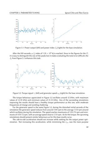
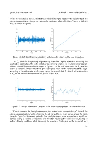
![CHAPTER 5. PARAMETER TUNING Ignasi Cifre and Àlex Garcia
optimized for the initial set of alphas, then the objective behind them is avoiding negative effects
on this acceleration while improving the ass and smoothing the power output.
Another aspect to check is the blade pitch angle with time. This angle will usually vary
between 12 and 18 degrees, as seen in Figure 5.4, aiming to reduce or increase the power gained
from wind flow. The pitch actuator varies the angle to capture more or less power from the wind,
depending on the actual and the desired value of Pe. However, the pitch angle is only checked to
ensure that the control is working properly, then by how much does it change is a non-essential
factor.
As a useful tool for succeeding comparison purposes, the results of both this part and from
the baseline simulation will be summarized. In Table 5.2 and Table 5.3 different elements to
analyse, such as the indices and the maximum and minimum peaks, are shown.
Table 5.2: Indices results for base and baseline simulations.
Jp [kJ] Jass [m/s] Jafa [m/s]
Base 5.26 × 10⁶
3293.1 6115.6
Baseline 9.28 × 10⁶
4698 6321.1
Table 5.3: Power and ass results for base and baseline simulations.
Pmax [kW] Pmin [kW] ass max [m/s2
] ass min [m/s2
]
Base 5347.13 4627.23 0.272 -0.269
Baseline 5392.16 3826.56 0.305 -0.349
Next step
Once the main results for the initial set of alphas are exposed, it is time to start with the param-
eter tuning simulations, according to that mentioned in the above methodology part.
5.3 First set of simulations
This first set of twelve simulations is divided into four parts. In each part, three values for one of
the alphas are tested. The combinations of values in each simulation are specified in Table 5.4.
This is the first approach for parameter tuning, and it must be ensured that the values tested
differ substantially from the original ones while the order of magnitude is maintained. The
values for each alpha are chosen mostly due to its order of magnitude. In Table 5.4 we can see
the different combinations executed in the first set of simulations. For each of the four alphas,
there is a value lower than the original one, a higher one, and a third one which is close to the
original value, in order to make comparisons with a similar value to that initial one.
62](https://image.slidesharecdn.com/d5dea01b-1c58-4cb9-b6c8-8c7a99c48f71-161121112012/85/BACHELOR_THESIS_ACCELERATIOM-BASED_CONTROL_OF_OFFSHORE_WT-74-320.jpg)

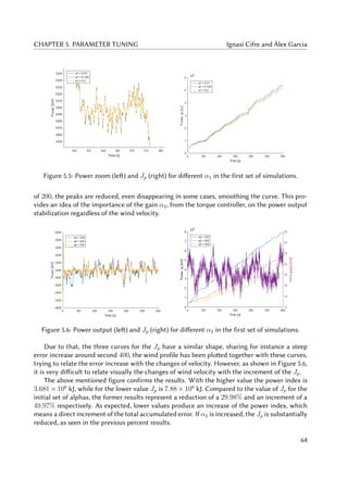


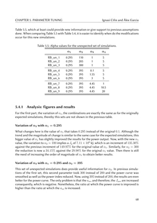
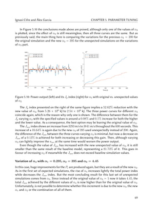

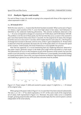
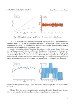
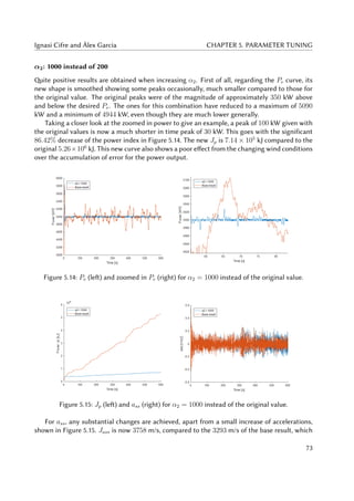
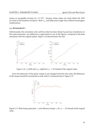
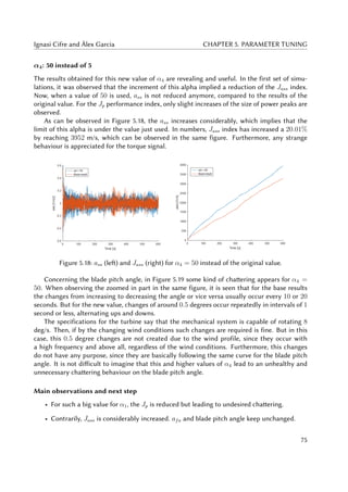

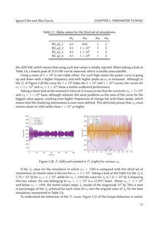
![CHAPTER 5. PARAMETER TUNING Ignasi Cifre and Àlex Garcia
Figure 5.21: Jp (left) and real generator torque τr for various α2.
For α2 = 0.01, in which the Pe is unable to reach the desired 5000 kW, the torque control is not
even working. The torque is constant throughout the simulation, which means that the blade
pitch angle is the only one working on the control system. For the other values, the same high
frequencies due to chattering obtained for the Pe curve are observed here, and at the same time
these torque curves are limited by the saturation torque of 47402.9 Nm, increasing the error
consequentially.
Table 5.8: Power results for different values of α2 in the third set of simulations.
α2 High peak [kW] Low peak [kW] Jp [kJ] Jp in %
0.01 4934 3410 6.84 × 10⁷
1302.85
1 × 10⁴
5028 4971 5.79 × 10⁵
11.01
1 × 10⁵
5531 4476 1.02 × 10⁷
193.92
1 × 10⁶
7007 3003 2.58 × 10⁷
490.49
Figure 5.22 shows that the accumulated error is extremely high for the first value tested, and
that for the other ones, the lower the value of α2, the lower the accumulated error. Since this is
the exact opposite trend of the first set of simulations, this supports the former conclusion that
the good range of this parameter lies between 1000 and 1 × 10⁴
, at least according to the power
output.
Concerning ass, similar conclusions come out. It can be seen in Figure 5.22 that with these
high values used now, the acceleration peaks are not below 0.25 m/s2
anymore, reaching values
near to 0.6 m/s2
, as expressed in Table 5.9. The higher the value of α2, the higher the acceleration
and, thus, the Jass index. Moreover, this table confirms what is not possible to see on the right
side of Figure 5.22, that for α2 = 1×10⁴
the lowest accumulated error is achieved. This supports
the hypothesis that the α2 value must remain somewhere under 1 × 10⁴
.
Recovering the value for Jass of 3758 m/s when α2 = 1000, the percentage that it represents
over the Jass value of the base simulation is a 114.12%. Comparing this result with those of the
78](https://image.slidesharecdn.com/d5dea01b-1c58-4cb9-b6c8-8c7a99c48f71-161121112012/85/BACHELOR_THESIS_ACCELERATIOM-BASED_CONTROL_OF_OFFSHORE_WT-90-320.jpg)
![Ignasi Cifre and Àlex Garcia CHAPTER 5. PARAMETER TUNING
Table 5.9: ass results for different values of α2 in the third set of simulations.
α2 High peak [m/s2
] Low peak [m/s2
] Jass [m/s] Jass in %
0.01 0.552 -0.424 4043 122.77
1 × 10⁴
0.578 -0.443 3791 115.12
1 × 10⁵
0.553 -0.457 4866 147.76
1 × 10⁶
0.574 -0.581 8170 248.10
fifth column in Table 5.9, it turns out to be the lowest Jass increment achieved. This implies that
although α2 affects the Jass, its effect is much lower than that on the Jp.
As observed in the Jass percentages, both for higher than α2 = 1 × 10⁴
and lower than
α2 = 1000 values the percentage of Jass over the one of the original base result is much higher
than 100%, adding more reasons for narrowing the range of α2.
The peak values shown both in Table 5.8 and Table 5.9 are the ones taken after the first 10
seconds of the simulation, since in the initial stage certain aspects from the initialization process
lead to some unrealistic peaks.
Figure 5.22: ass (left) and Jass (right) for various α2.
When it comes to afa, an unexpected result is obtained. Contrarily to other results, this
acceleration is not much affected by this variation of values. This is proved in Figure 5.23 since
the different curves are seen and all the peaks have a similar size, around 0.5 m/s2
.
On the right side, it is possible to understand what occurs with α2 = 0.01 for the power
output. Some kind of deviation of 1 degree is appreciated for the blade pitch angle, which seems
to be the cause for the stabilization of the power around 4000 kW instead of 5000 kW.
Main observations and next step
• For α2 = 0.01 the system is unable to provide the desired power. The blade pitch angle
has changed.
79](https://image.slidesharecdn.com/d5dea01b-1c58-4cb9-b6c8-8c7a99c48f71-161121112012/85/BACHELOR_THESIS_ACCELERATIOM-BASED_CONTROL_OF_OFFSHORE_WT-91-320.jpg)

![Ignasi Cifre and Àlex Garcia CHAPTER 5. PARAMETER TUNING
has been proved that should not exceed 50, the test values will be 5, 20, 35 and 50. The resulting
combinations are those expressed in Table 5.10.
Table 5.10: Alpha values for the fourth set of simulations.
α1 α2 α3 α4
R4_11 0.1 500 1 5
R4_12 0.1 500 1 20
R4_13 0.1 500 1 35
R4_14 0.1 500 1 50
R4_21 0.1 750 1 5
R4_22 0.1 750 1 20
R4_23 0.1 750 1 35
R4_24 0.1 750 1 50
R4_31 0.1 1000 1 5
R4_32 0.1 1000 1 20
R4_33 0.1 1000 1 35
R4_34 0.1 1000 1 50
R4_41 0.1 1250 1 5
R4_42 0.1 1250 1 20
R4_43 0.1 1250 1 35
R4_44 0.1 1250 1 50
The combination of this two parameters is issued to smooth the power curve, and thereby,
reduce the total accumulated error, with the effects of α2, and use α4 to counteract the increment
of the accumulated ass. The range of values used for each gain has been designed according to
the results of previous simulations.
5.7.1 Analysis: figures and results
For the exposition of results, four different curves will be represented for each figure. One curve
will be the one using the baseline control model from [Jonkman et al. (2009)], this is without the
STA-based control system, and another curve will be the one for the base result. The other two
curves will be, out of the sixteen different simulations in this fourth set, the combination that
provides the better Pe results, and finally comes the combination that provides the better results
for the ass.
Power output
The improvement on the last simulations, compared to the baseline and base results, is remark-
able and easy to see in Figure 5.25. The curves for the combination that minimizes the Jp and the
81](https://image.slidesharecdn.com/d5dea01b-1c58-4cb9-b6c8-8c7a99c48f71-161121112012/85/BACHELOR_THESIS_ACCELERATIOM-BASED_CONTROL_OF_OFFSHORE_WT-93-320.jpg)
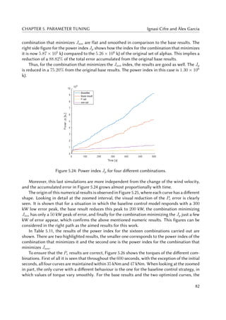
![Ignasi Cifre and Àlex Garcia CHAPTER 5. PARAMETER TUNING
Figure 5.25: Pe (left) and zoomed in Pe (right) for four different combinations.
Figure 5.26: Realt torque τr (left) and zoomed in real torque (right) for four different combina-
tions.
changes of torque are clearly marked with ups and downs. For the optimized power curve and
optimized ass curve, the frequency of change is somewhat higher than for the base results, but
with similar behaviours overall. None of the previous chattering issues are observed.
Acceleration ass
In Figure 5.27 is clearly seen that all other curves are seen above and below the curve that op-
timizes ass. However, the original set of alphas from [Tutivén et al. (2015)] is the combination
reducing at its most the total accumulated ass. This implies that there is always a correlation
between the output power and ass, and the difficulty remains behind finding the equilibrium
between the reduction of the first and avoiding the second from increasing.
In Table 5.12, for each of the sixteen combinations Jass results are shown. Again, both high-
lighted numbers correspond to the combination that minimizes the Jass and the one that mini-
mizes the Jp. The combination with α2 = 750 and α4 = 35 increases a 6.3% the total accumu-
83](https://image.slidesharecdn.com/d5dea01b-1c58-4cb9-b6c8-8c7a99c48f71-161121112012/85/BACHELOR_THESIS_ACCELERATIOM-BASED_CONTROL_OF_OFFSHORE_WT-95-320.jpg)
![CHAPTER 5. PARAMETER TUNING Ignasi Cifre and Àlex Garcia
Table 5.11: Power index for each combination of α2 and α4.
α4 = 5 α4 = 20 α4 = 35 α4 = 50
α2 = 500 1.96 × 10⁶
2.06 × 10⁶
2.32 × 10⁶
2.59 × 10⁶
α2 = 750 1.04 × 10⁶
1.10 × 10⁶
1.30 × 10⁶
1.54 × 10⁶
α2 = 1000 7.14 × 10⁵
7.66 × 10⁵
9.25 × 10⁵
1.12 × 10⁶
α2 = 1250 5.88 × 10⁵
6.16 × 10⁵
7.73 × 10⁵
9.20 × 10⁵
lated ass error, while the combination with α2 = 1250 and α4 = 5 increases a 15.67% the Jass,
both in comparison with the results of the original set of alphas.
Table 5.12: Jass index for each combination of α2 and α4 [in kJ].
α4 = 5 α4 = 20 α4 = 35 α4 = 50
α2 = 500 3913.6 3745.0 3541.1 3876.0
α2 = 750 3805.9 3693.1 3500.6 3904.7
α2 = 1000 3758.2 3693.9 3526.9 3905.9
α2 = 1250 3809.2 3716.5 3560.2 3921.2
Even though the results are worse than the base result, they still imply a Jass reduction of a
25.48% and a 18.91% respectively, in comparison to the results of the baseline. Since the baseline
is the standard case for the FAST simulation, it means that the values of acceleration obtained
are perfectly applicable.
Figure 5.27: ass (left) and Jass (right) for four different combinations.
84](https://image.slidesharecdn.com/d5dea01b-1c58-4cb9-b6c8-8c7a99c48f71-161121112012/85/BACHELOR_THESIS_ACCELERATIOM-BASED_CONTROL_OF_OFFSHORE_WT-96-320.jpg)

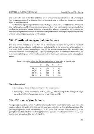
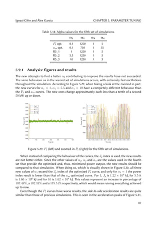


![Ignasi Cifre and Àlex Garcia CHAPTER 6. RESULTS ANALYSIS
Table 6.1: Optimal range for each of the α gains.
α1 α2 α3 α4
[0.1, 0.3] [750, 1250] [1, ?] [5, 40]
best combinations of α gains are the ones achieved in the fourth set of simulations instead of
the final set of simulations performed.
In the following parts, the results that have already been shown in Table 5.11 and Table 5.12
for Jp and Jass are going to be treated. In the following tables, the percentages of increase or
reduction respect to the base results and respect to the baseline results in some cases will be
obtained.
6.3.1 Improvements achieved
Jp reduction
The improvement corresponding to the first guideline comes first. Having the power stabilization
and smoothness as the first objective has been well-accomplished. Comparing the Jp index
values with that of the base result, the following percentages of reduction expressed in Table 6.2
are obtained.
The highest reduction arises from the combination with α2 = 1250 and α4 = 5, with a
reduction of a 88.82%, closely followed by α2 = 1250 and α4 = 20 with a reduction of 88.29%.
When observing carefully all the reductions, there is a clear tendency showing that the highest
values are placed close to the bottom left corner of Table 6.2. This is for high values of α2 and
low values of α4. However, any of the combinations with α2 = 1250 provides reductions higher
than 80%.
Table 6.2: Jp reduction in percentage, Jp of each combination of α2 and α4 over the base result.
α4 = 5 α4 = 20 α4 = 35 α4 = 50
α2 = 500 62,75% 60,74% 55,86% 50,69%
α2 = 750 80,18% 79,03% 75,20% 70,72%
α2 = 1000 86,42% 85,42% 82,40% 78,70%
α2 = 1250 88,82% 88,29% 85,30% 82,51%
Aiming to identify the trend, it is seen that within this range of α2, for any of their values
the percentage of reduction decreases as α4 increases. Similarly, for any of the values of α4, it is
seen that the percentage of reduction increases as α2 is increased. As a consequence, it is easy
to understand that the highest reduction is for the highest α2 and lowest α4, and exactly the
opposite occurs for the lowest reduction, which anyway achieves a 50.69% of reduction.
93](https://image.slidesharecdn.com/d5dea01b-1c58-4cb9-b6c8-8c7a99c48f71-161121112012/85/BACHELOR_THESIS_ACCELERATIOM-BASED_CONTROL_OF_OFFSHORE_WT-105-320.jpg)

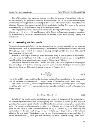

![Ignasi Cifre and Àlex Garcia CHAPTER 6. RESULTS ANALYSIS
Table 6.7: Summary of results for the best combinations.
Combination α2 = 1250 α2 = 750 α2 = 1250 α2 = 1250
α4 = 5 α4 = 35 α4 = 35 α4 = 20
Best for: Jp Jass I1 I2
Jp [kJ] 5.88 × 10⁵
1.30 × 10⁶
7.73 × 10⁵
6.16 × 10⁵
Jass [m/s] 3809.2 3500.6 3560.2 3716.5
Jp [-] 88.82% 75.20% 85.30% 88.29%
Jass [-] 18.92% 25.49% 24.22% 20.89%
I1 [-] 1.680 1.917 2.066 1.845
I2 [-] 67.85 60.29 66.98 68.07
6.3.3 Optimal set of alphas: figures and results
In the fourth section, the results for the optimal combination were not plotted. Here, to ensure
that the selected combination of alphas does not suffer any strange behaviours in any of the
results, the different types of figures that have been checked during the parameter tuning process
will be shown for the optimal combination. In the figures, this combination will be compared
with the base simulation combination.
First of all, the power output Pe is shown for the two combinations in Figure 6.1. This is
probably the figure that represents better where do we have put our efforts. The new curve
has a definitely improved tracking error performance, is well-stabilized, almost invariable with
the wind conditions, and almost all the previous peaks from the base simulation curve are now
perfectly smoothed.
The peaks for this optimal combination are now 5047 kW and 4957 kW, only less than 50 kW
above or below the desired value, and far from the previous 5347 kW and 4627 kW of the base
result.
To ensure that no chattering occurs, the Figure 6.2 shows an interval of 100 seconds of the
simulation. In this part it can be observed in more detail that the shapes that this optimal
combination curve presents is very flat, but when any variations occur, coinciding with the peaks
of the base results curve, any behaviours of high frequencies or chattering appear, or at least the
frequencies of change are of the same size, thereby making the results valid. Moreover, this
closer view provides a better approach to compare the duration and size of the peaks for the two
curves.
For the Jp results, anything new is said since we have been working with this result and
the reduction that implies throughout this chapter. However, it is worth mentioning that the
accumulation of error grows now almost proportionally with time and that most part of this
values is due to the strange disturbances that we have for the initial seconds. Anyway, the
figure gives a visual idea of the size of the reduction.
Regarding the torque behaviour seen in Figure 6.3, it is seen that the torque for the optimal
results follows similar τr values, but instead of clearly marked ups and downs as for the base
result, the transition now from increasing to decreasing the torque and vice versa has a much
97](https://image.slidesharecdn.com/d5dea01b-1c58-4cb9-b6c8-8c7a99c48f71-161121112012/85/BACHELOR_THESIS_ACCELERATIOM-BASED_CONTROL_OF_OFFSHORE_WT-109-320.jpg)
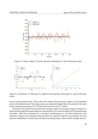
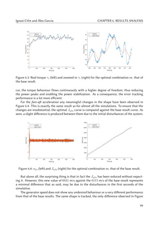
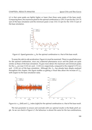
![Ignasi Cifre and Àlex Garcia CHAPTER 6. RESULTS ANALYSIS
since the optimal combination tracks the performance of the base simulation with only slight
differences such as a small increase of the peaks.
Figure 6.7: Blade pitch angle (left) and zoomed in blade pitch angle (right) for the optimal com-
bination vs. that of the base result.
However, when checking the zoomed in part, some changes with ups and downs of around a
tenth of degree are observed for the optimal results. Even though this changes do not corrupt the
mechanical limits of the rate of 8 deg/s, and do not correspond to chattering either. As expected,
this behaviour is due to the new value used for α4, that tries to reduce the ass by tracking more
accurately the blade pitch angle.
Finally, the main outcomes for this chosen best combination are presented in Table 6.8, com-
pared with the results of the base simulation.
Table 6.8: Results of the optimal vs base results.
Base Optimal
Combination α2 = 200, α4 = 5 α2 = 1250, α4 = 20
High peak [kW] 5347.13 5047.73
Low peak [kW] 4627.23 4957.17
Jp [kJ] 5.26 × 10⁶
6.16 × 10⁵
Jp [-] - 88.29%
High peak [m/s2
] 0.272 0.248
Low peak [m/s2
] -0.269 -0.238
Jass [m/s] 3293.10 3716.50
Jass [-] 29.90% 20.89%
101](https://image.slidesharecdn.com/d5dea01b-1c58-4cb9-b6c8-8c7a99c48f71-161121112012/85/BACHELOR_THESIS_ACCELERATIOM-BASED_CONTROL_OF_OFFSHORE_WT-113-320.jpg)
![CHAPTER 6. RESULTS ANALYSIS Ignasi Cifre and Àlex Garcia
6.3.4 Numerical issues
Along the parameter tuning process, a lot of combinations have given results which we have
rejected due to the chattering phenomena and high frequency components observed. Once we
have decided for the optimal combination, most of its figures have been zoomed in and examined
with determination, aiming to ensure that any undesired effects are produced.
For the Pe in Figure 6.1, a strange behaviour is observed when zooming in deeply. The Figure
6.8 shows it, although it is important to look at the interval shown, which is for less than 4
seconds. This implies that this behaviour is very small in size and duration, even though it is
repeated constantly along the simulation.
After some research, it has been concluded that this can be explained as numerical issues,
which are treated in detail in [Pozo et al. (2008)]. They usually occur in uncertain systems with
complex algorithms in the mathematical formulation and in the numerical implementation.
As explained there, the control of the system needs to:
(i) measure the output in order to feedback the system,
(ii) solve the differential equations involved, such as Equation (2.14) and Equation (2.16) to
estimate the parameters of the system, and
(iii) process the control system.
Due to these steps that the computational problem involves, several numerical errors may ap-
pear:
(i) measurement errors when measuring the output,
(ii) errors due to the numerical integration of the differential equations, and
(iii) errors in floating-point arithmetic when processing the control system.
Once explained why do these numerical issues appear, they can be easily identified in Fig-
ure 6.8 for the optimal curve that we have obtained. But even though the base result curve is
implemented using the same control strategy, this numerical errors do not appear for this curve.
The reason why this happens is because some design parameters can be amplifiers of this
errors. In our case, α2 is the variable that has created this numerical errors by increasing the
value of this gain. Taking a closer look at the zoomed in Pe, around 20 peaks are identified in
less than 0.3 seconds. The frequency of this peaks then corresponds quite well to the sampling
rate of the system of 0.01 seconds, and thereby, it ensures that this high frequency components
have a numerical origin.
These numerical errors are negligible due to their size and would not suppose any problem to
our system, they only indicate the numerical complexity of the control strategy. However, they
should be avoided as much as possible since their increase could damage the actuators involved
because of their working rates and compromise the stability of the system.
In other cases of this work, high frequency components have been identified as well, but
with much greater peaks. Furthermore, those peaks have not corresponded with the sampling
102](https://image.slidesharecdn.com/d5dea01b-1c58-4cb9-b6c8-8c7a99c48f71-161121112012/85/BACHELOR_THESIS_ACCELERATIOM-BASED_CONTROL_OF_OFFSHORE_WT-114-320.jpg)
![Ignasi Cifre and Àlex Garcia CHAPTER 6. RESULTS ANALYSIS
Figure 6.8: Numerical errors in the zoomed in Pe for the optimal combination vs. that of the base
result.
rate, and that is the reason why they are understood as part of the dynamics of the system. In
that case the problems do not have the origin on numerical computations and the power output
signal is clearly corrupted by high frequencies independent from these numerical errors.
6.4 Further development
After analysing in detail the best results achieved, several ideas come to mind about how would
we set the pathway for further improvement. These ideas are explained in a priority order.
First of all, trying to reduce the Jp index as much as possible making sure that the Jass is
still equal or below the baseline simulation Jass value. To reach this goal the trend is clearly
rising the gain in the control equations responsible for the largest improvements. Thus, the
design parameter α2 value should be raised above the highest value producing good results tried,
1250, but much below 1 × 10⁴
. Consequently, the range of values that we would test for α2 is
[1250, 2500].
For α4, the trend has not been possible to identify evidently. It is clear that values either
below α4 = 5 or above α4 = 50 should be avoided, either because the Jass is not reduced or
because chattering and undesired behaviours in the blade pitch angle occur. What we would
probably do is narrowing the range already used and testing more values within this range since
any trend exists, thereby, the most effective way is performing more simulations. The range
would probably be [15, 40].
Some more time could be spent on α1. Even though their effects are only lightly substantial,
it could be worth trying to narrow the range of it, and knowing that below α1 = 0.1 or above
α1 = 1 the results provided are not desirable, the new range to explore more deeply would be
103](https://image.slidesharecdn.com/d5dea01b-1c58-4cb9-b6c8-8c7a99c48f71-161121112012/85/BACHELOR_THESIS_ACCELERATIOM-BASED_CONTROL_OF_OFFSHORE_WT-115-320.jpg)
![CHAPTER 6. RESULTS ANALYSIS Ignasi Cifre and Àlex Garcia
[0.1, 0.5].
Finally, for α3 we would not develop any more investigation due to the lack of its influence
and results. Instead, we would try to remove it from the control equations in order to check
whether the control strategy keeps working as desired or not.
6.5 Approach on a real-implementation
To correctly understand all the benefits that the achievements of this work would provide, a
complete study implementing this control system in a real wind should be performed accurately.
Since it is not the aim of this thesis to do so, only a superficial approximation is carried out here.
This simple study only takes into account the main goal of the power stability, without deepening
in the mechanical vibrations.
We will take as an example the offshore wind power plant Horns Rev in Denmark, of 160 MW.
Although it is composed of 80 units of 2 MW, we will assume that is composed of 32 units of the
used NREL 5 MW wind turbine from this work. The turbines are distributed, as in the real case,
as an obliqued rectangle, with horizontal and vertical rows.
Recalling the results for our optimal combination compared to the base simulation and the
baseline simulation results, found in 6.9, we will accumulate the differences obtained between
the different combinations taking into account all the wind turbine units of the plant. Those are
separated 560 m in both directions in the real case. Due to the size of our turbines, this distance
would be even greater, meaning that all the wind turbines would receive similar wind conditions
but not the same wind velocities would act in each wind turbine at a time.
Thereby, Table 6.9 considers the worst case for the biggest differences of the peaks, occurring
around the second 134 for the maximum peak and second 395 for the minimum peak:
Table 6.9: Differences in kW between optimal, baseline and base combinations in specific worst
moments of the power stability.
Optimal Baseline Base
High peak [kW] 5047.73 5392.16 5347.13
Difference [kW] - 344.43 299.4
Accumulated [kW] - 11017.6 9580.8
Low peak [kW] 4957.17 3826.56 4627.23
Difference [kW] - 1130.61 329.94
Accumulated [kW] - 36179.52 10558.08
The accumulated error in the peaks from this table involve multiplying the power difference
by the 32 turbines of the wind farm. It must be said that these are cases that could hardly
ever occur, since although the wind conditions are real, each wind turbine would have slightly
different wind velocities, thus implying that the peaks would not necessarily occur at the same
time.
104](https://image.slidesharecdn.com/d5dea01b-1c58-4cb9-b6c8-8c7a99c48f71-161121112012/85/BACHELOR_THESIS_ACCELERATIOM-BASED_CONTROL_OF_OFFSHORE_WT-116-320.jpg)


![References
Bibliographic references
[Sawyer and Reve (2016)] Sawyer, S. and K. Reve. Abril 2016. Global wind report: Anual Market
Update. Brussels: Global Wind Energy Council (GWEC).
[IEA (2015)] International Energy Agency (IEA). 2016. World Energy Outlook. Paris: Interna-
tional Energy Agency.
[Bailey et al. (2014)] Bailey H., P.M. Thompson, and K.L. Brookes. September 2014. “Assessing
Environmental Impacts of Offshore Wind Farms: Lessons Learned and Recommendations
for the Future.” Bailey et al. Aquatic Biosystems 10:8.
[Office of Energy and Renewable Energy (2016)] Office of Energy and Renewable Energy, U.S
Department of Energy. 2016. http://www.eere.energy.gov/windandhydro/wind_how.html.
Accessed May 20.
[Pao L.Y. and K.E. Johnson (2009)] Pao L.Y. and K.E. Johnson. 2009. “A Tutorial on the Dynamics
and Control of Wind Turbines and Wind Farms.” In Proceedings of the 2009 American
Control Conference (ACC), St. Louis , MO, USA, June 10—12.
[NREL (2016)] National Renewable Energy Laboratory (NREL). 2016. “NTWC Information Por-
tal.” Accesed March 23. https://nwtc.nrel.gov/FAST.
[Jonkman et al. (2009)] Jonkman J., S.Butterfield, W. Musial, and G. Scott. 2009. “Definition of a
5-MW Reference Wind Turbine for Offshore System Development.” NREL: Technical Report
NREL/TP-500-38060.
[Tutivén et al. (2015)] Tutivén C., Y. Vidal, J. Rodellar, and L. Acho. 2015. “Acceleration-based
fault tolerant control design of offshore fixed wind turbines.” Struct. Control Health Monit.
00:1—15.
[Odgaard and Johnson (2013)] Odgaard P., K. Johnson. 2013 “Wind Turbine Fault Diagnosis and
Fault Tolerant Control–An Enhanced Benchmark Challenge.” In Proceedings of the 2013
American Control Conference (ACC), Washington, DC, USA, June 17—19.
113](https://image.slidesharecdn.com/d5dea01b-1c58-4cb9-b6c8-8c7a99c48f71-161121112012/85/BACHELOR_THESIS_ACCELERATIOM-BASED_CONTROL_OF_OFFSHORE_WT-125-320.jpg)
![REFERENCES Ignasi Cifre and Àlex Garcia
[Odgaard et al. (2009)] Odgaard P., J. Stourstrup, and M. Kinnaert. 2009. “ Fault toerant control
of wind turbines, a benchmark model.” Proc 7th IFAC Symposium on Fault Detection,
Supervision and Safety of Technical Processes, Barcelona, Spain, 155—160.
[Smith (2006)] Smith S. W. 2006. “The Scientist and Engineer’s Guide to Digital Signal Process-
ing.” San Diego, CA: California Technical Publishing, 2006.
[Strum and Kirk (2000)] Strum R.D., D. E. Kirk. 2000. “Contemporany Linear Systems Using
MATLAB®
.” Brooks/Cole, Pacific Grove, CA, USA, 2000, 221—297.
[Jonkman and Buhl (2005)] Jonkman J., M. L. Buhl Jr. 2005. “FAST User’s Guide.” NREL: Tech-
nical Report NREL/EL-500-38230.
[Jonkman and Jonkman (2016)] Jonkman B., J. Jonkman. 2016. “FAST v8 guide: FAST v8.15.00a-
bjj.” NREL.
[Jonkman et al. (2012)] Jonkman J., A. Robertson et al. 2012. “Offshore Code Comparison Col-
laboration Continuation (OC4), Phase I—Results of Coupled Simulations of an Offshore
Wind Turbine with Jacket Support Structure.” To be presented at the 22nd
International
Society of Offshore and Polar Engineers Conference, Rhodes, Greeces, June 17.
[Pozo et al. (2008)] Pozo F., F. Ikhouane, J. Rodellar. 2008 “Numerical issues in backstepping
control: Sensitivity and parameter tuning”. Journal of the Franklin Institute 345: 891—905.
Consulting bibliography
[Edwards and Spurgeon (1998)] Edwards C., S. K. Spurgeon. Sliding Mode Control: Theory and
Applications (Florida: Taylor & Francis group, 1998).
[Slotine and Li (1998)] Slotine J.J. E., W. Li. Applied Nonlinear Control (New Jersey: Prentice-Hall,
Inc., 1991).
114](https://image.slidesharecdn.com/d5dea01b-1c58-4cb9-b6c8-8c7a99c48f71-161121112012/85/BACHELOR_THESIS_ACCELERATIOM-BASED_CONTROL_OF_OFFSHORE_WT-126-320.jpg)


![Budget
This chapter contains the budget of the Bachelor’s thesis. Our thesis is a theoretical thesis, that
only involves research and simulation, and so it does not have any type of building or installation,
neither materials nor working machines. Due to that fact, the budget in this thesis is not an
important part. Consequently, it has not been cited in the report and the values obtained in this
chapter are not used.
Table 7.1 contains the calculations and the costs of the thesis that have been developed. It
includes the name of each of the items considered, the number of items used, the cost of each
of them, and the total cost considering all the items set.
Table 7.1: Thesis budget.
Concept No. of items [-] Individual cost [e] Total cost [e]
Software licenses
FAST software 1 0 0
MATLAB®
2 400 800
Texworks 1 0 0
Working hours 1440 36 51840
Thesis report 1 60 60
Office equipment
Working station 1 2800 2800
Laptop 2 600 1200
Total 56300
119](https://image.slidesharecdn.com/d5dea01b-1c58-4cb9-b6c8-8c7a99c48f71-161121112012/85/BACHELOR_THESIS_ACCELERATIOM-BASED_CONTROL_OF_OFFSHORE_WT-131-320.jpg)

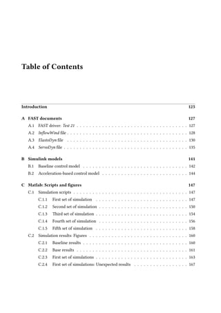


![APPENDIX A. FAST DOCUMENTS Ignasi Cifre and Àlex Garcia
22 −−−−−−−−−−−−−−−−−−−−−− INPUT FILES −−−−−−−−−−−−−−−−−−−−−−−−−−−−−−−−−−−−−−−−−−−
23 "5 MW_Baseline / NRELOffshrBsline5MW_OC4Jacket_ElastoDyn . dat " EDFile
− Name of f i l e containing ElastoDyn input parameters ( quoted s t r i n g )
24 "5 MW_Baseline / NRELOffshrBsline5MW_BeamDyn . dat " BDBldFile ( 1 ) − Name of
f i l e containing BeamDyn input parameters f o r blade 1 ( quoted s t r i n g )
25 "5 MW_Baseline / NRELOffshrBsline5MW_BeamDyn . dat " BDBldFile ( 2 ) − Name of
f i l e containing BeamDyn input parameters f o r blade 2 ( quoted s t r i n g )
26 "5 MW_Baseline / NRELOffshrBsline5MW_BeamDyn . dat " BDBldFile ( 3 ) − Name of
f i l e containing BeamDyn input parameters f o r blade 3 ( quoted s t r i n g )
27 "5 MW_Baseline / NRELOffshrBsline5MW_InflowWind_12mps . dat " I n f l o w F i l e −
Name of f i l e containing inflow wind input parameters ( quoted s t r i n g )
28 "5 MW_Baseline / NRELOffshrBsline5MW_OC4Jacket_AeroDyn . dat " A e r o F i l e −
Name of f i l e containing aerodynamic input parameters ( quoted s t r i n g )
29 "5 MW_Baseline / NRELOffshrBsline5MW_OC4Jacket_ServoDyn . dat " S e r v o F i l e −
Name of f i l e containing c o n t r o l and e l e c t r i c a l −d r i v e input parameters (
quoted s t r i n g )
30 "5 MW_Baseline / NRELOffshrBsline5MW_OC4Jacket_HydroDyn . dat " HydroFile −
Name of f i l e containing hydrodynamic input parameters ( quoted s t r i n g )
31 "5 MW_Baseline / NRELOffshrBsline5MW_OC4Jacket_SubDyn . dat " SubFile −
Name of f i l e containing sub−s t r u c t u r a l input parameters ( quoted s t r i n g )
32 " unused " MooringFile − Name of f i l e containing mooring system input
parameters ( quoted s t r i n g )
33 " unused " I c e F i l e − Name of f i l e containing i c e input parameters (
quoted s t r i n g )
34 −−−−−−−−−−−−−−−−−−−−−− OUTPUT −−−−−−−−−−−−−−−−−−−−−−−−−−−−−−−−−−−−−−−−−−−−−−−−
35 True SumPrint − P r i n t summary data to " <RootName > . sum" ( f l a g )
36 1 SttsTime − Amount of time between screen s t a t u s messages
( s )
37 99999 ChkptTime − Amount of time between c r e a t i n g checkpoint
f i l e s f o r p o t e n t i a l r e s t a r t ( s )
38 0 . 0 5 DT_Out − Time step f o r t a b u l a r output ( s ) ( or " d e f a u l t
" )
39 0 TStart − Time to begin t a b u l a r output ( s )
40 2 OutFileFmt − Format f o r t a b u l a r ( time−marching ) output f i l e
( switch ) { 1 : t e x t f i l e [ <RootName > . out ] , 2 : binary f i l e [ <
RootName > . outb ] , 3 : both }
41 True TabDelim − Use tab d e l i m i t e r s in t e x t t a b u l a r output f i l e
? ( f l a g ) { uses spaces i f f a l s e }
42 " ES10 . 3 E2 " OutFmt − Format used f o r t e x t t a b u l a r output , excluding
the time channel . R e s u l t i n g f i e l d should be 10 c h a r a c t e r s . ( quoted
s t r i n g )
A.2 InflowWind file
1
2 −−−−−−− InflowWind v3 . 0 1 . ∗ INPUT FILE
−−−−−−−−−−−−−−−−−−−−−−−−−−−−−−−−−−−−−−−−−−−−−−−−−−−−−−−−−−−−−−−−−−−−−−−−−
3 12 m/ s t u r b u l e n t winds on 31 x31 FF g r i d and tower f o r FAST CertTests #18 , #19 ,
#21 , #22 , #23 , and #24
128](https://image.slidesharecdn.com/d5dea01b-1c58-4cb9-b6c8-8c7a99c48f71-161121112012/85/BACHELOR_THESIS_ACCELERATIOM-BASED_CONTROL_OF_OFFSHORE_WT-140-320.jpg)
![Ignasi Cifre and Àlex Garcia APPENDIX A. FAST DOCUMENTS
4 −−−−−−−−−−−−−−−−−−−−−−−−−−−−−−−−−−−−−−−−−−−−−−−−−−−−−−−−−−−−−−−−−−−−−−−−−−
5 F a l s e Echo − Echo input data to <RootName > . ech ( f l a g )
6 4 WindType − switch f o r wind f i l e type (1= steady ; 2= uniform ;
3= binary TurbSim FF ; 4= binary Bladed−s t y l e FF ; 5=HAWC format ;
6= User defined )
7 0 PropogationDir − D i r e c t i o n of wind propogation ( m e t e o r o l i g i c a l
r o t a t i o n from aligned with X ( p o s i t i v e r o t a t e s towards −Y ) −−
degrees )
8 1 NWindVel − Number of points to output the wind v e l o c i t y (0
to 9)
9 0 WindVxiList − L i s t of c o o r d i n a t e s in the i n e r t i a l X d i r e c t i o n
(m)
10 0 WindVyiList − L i s t of c o o r d i n a t e s in the i n e r t i a l Y d i r e c t i o n
(m)
11 90 WindVziList − L i s t of c o o r d i n a t e s in the i n e r t i a l Z d i r e c t i o n
(m)
12 ================== Parameters f o r Steady Wind Conditions [ used only f o r
WindType = 1] =========================
13 0 HWindSpeed − Horizontal windspeed
14 90 RefHt − Reference height f o r h o r i z o n t a l wind speed
15 0 . 2 PLexp − Power law exponent
16 ================== Parameters f o r Uniform wind f i l e [ used only f o r WindType
= 2] ============================
17 " Wind /90 m_12mps_twr . bts " Filename − Filename of time s e r i e s data f o r
uniform wind f i e l d .
18 90 RefHt − Reference height f o r h o r i z o n t a l wind speed
19 1 25 . 8 8 RefLength − Reference length f o r l i n e a r h o r i z o n t a l and
v e r t i c a l sheer
20 ================== Parameters f o r Binary TurbSim Full −F i e l d f i l e s [ used only
f o r WindType = 3] ==============
21 " Wind /90 m_12mps_twr . bts " Filename − Name of the F u l l f i e l d wind f i l e
to use ( . bts )
22 ================== Parameters f o r Binary Bladed−s t y l e Full −F i e l d f i l e s [ used
only f o r WindType = 4] =========
23 " Wind /90 m_12mps " FilenameRoot − Rootname of the f u l l −f i e l d wind f i l e to
use ( . wnd , . sum )
24 F a l s e TowerFile − Have tower f i l e ( . twr ) [ f l a g ]
25 ================== Parameters f o r HAWC−format binary f i l e s [ Only used with
WindType = 5] =====================
26 " wasp Output basic_5u . bin " FileName_u − name of the f i l e containing
the u−component f l u c t u a t i n g wind
27 " wasp Output basic_5v . bin " FileName_v − name of the f i l e containing
the v−component f l u c t u a t i n g wind
28 " wasp Output basic_5w . bin " FileName_w − name of the f i l e containing
the w−component f l u c t u a t i n g wind
29 64 nx − number of g r i d s in the x d i r e c t i o n ( in the 3
f i l e s above )
30 32 ny − number of g r i d s in the y d i r e c t i o n ( in the 3
f i l e s above )
31 32 nz − number of g r i d s in the z d i r e c t i o n ( in the 3
f i l e s above )
129](https://image.slidesharecdn.com/d5dea01b-1c58-4cb9-b6c8-8c7a99c48f71-161121112012/85/BACHELOR_THESIS_ACCELERATIOM-BASED_CONTROL_OF_OFFSHORE_WT-141-320.jpg)
![APPENDIX A. FAST DOCUMENTS Ignasi Cifre and Àlex Garcia
32 16 dx − d i s t a n c e ( in meters ) between points in the x
d i r e c t i o n
33 3 dy − d i s t a n c e ( in meters ) between points in the y
d i r e c t i o n
34 3 dz − d i s t a n c e ( in meters ) between points in the z
d i r e c t i o n
35 90 RefHt − r e f e r e n c e height ; the height ( in meters ) of the
v e r t i c a l center of the g r i d
36 −−−−−−−−−−−−− S c a l i n g parameters f o r turbulence
−−−−−−−−−−−−−−−−−−−−−−−−−−−−−−−−−−−−−−−−−−−−−−−−−−−−−−−−−
37 1 ScaleMethod − Turbulence s c a l i n g method [0 = none , 1 =
d i r e c t scaling , 2 = c a l c u l a t e s c a l i n g f a c t o r based on a d e s i r e d
standard d e v i a t i o n ]
38 1 SFx − Turbulence s c a l i n g f a c t o r f o r the x d i r e c t i o n
( −) [ ScaleMethod =1]
39 1 SFy − Turbulence s c a l i n g f a c t o r f o r the y d i r e c t i o n
( −) [ ScaleMethod =1]
40 1 SFz − Turbulence s c a l i n g f a c t o r f o r the z d i r e c t i o n
( −) [ ScaleMethod =1]
41 12 SigmaFx − Turbulence standard d e v i a t i o n to c a l c u l a t e
s c a l i n g from in x d i r e c t i o n (m/ s ) [ ScaleMethod =2]
42 8 SigmaFy − Turbulence standard d e v i a t i o n to c a l c u l a t e
s c a l i n g from in y d i r e c t i o n (m/ s ) [ ScaleMethod =2]
43 2 SigmaFz − Turbulence standard d e v i a t i o n to c a l c u l a t e
s c a l i n g from in z d i r e c t i o n (m/ s ) [ ScaleMethod =2]
44 −−−−−−−−−−−−− Mean wind p r o f i l e parameters ( added to HAWC−format f i l e s )
−−−−−−−−−−−−−−−−−−−−−−−−−−−−−−−−−
45 5 URef − Mean u−component wind speed at the r e f e r e n c e
height [m/ s ]
46 2 WindProfile − Wind p r o f i l e type (0= constant ;1= logarithmic ,2=
power law )
47 0 . 2 PLExp − Power law exponent [−] ( used only when
WindProfile =2)
48 0 . 0 3 Z0 − Surface roughness length [m] ( used only when
WindProfile =1)
49 ====================== OUTPUT ================================
50 F a l s e SumPrint − P r i n t summary data to <RootName > . IfW . sum ( f l a g )
51 OutList − The next l i n e ( s ) contains a l i s t of output
parameters . See OutListParameters . x l s x f o r a l i s t i n g of
a v a i l a b l e output channels , ( −)
52 " Wind1VelX " X−d i r e c t i o n wind v e l o c i t y at point WindList ( 1 )
53 " Wind1VelY " Y−d i r e c t i o n wind v e l o c i t y at point WindList ( 1 )
54 " Wind1VelZ " Z−d i r e c t i o n wind v e l o c i t y at point WindList ( 1 )
55 END of input f i l e ( the word "END" must appear in the f i r s t 3 columns of t h i s
l a s t OutList l i n e )
56 −−−−−−−−−−−−−−−−−−−−−−−−−−−−−−−−−−−−−−−−−−−−−−−−−−−−−−−−−−−−−−−−−−−−−−−−−−−−−
130](https://image.slidesharecdn.com/d5dea01b-1c58-4cb9-b6c8-8c7a99c48f71-161121112012/85/BACHELOR_THESIS_ACCELERATIOM-BASED_CONTROL_OF_OFFSHORE_WT-142-320.jpg)
![Ignasi Cifre and Àlex Garcia APPENDIX A. FAST DOCUMENTS
A.3 ElastoDyn file
1
2 −−−−−−− ELASTODYN v1 . 0 3 . ∗ INPUT FILE
−−−−−−−−−−−−−−−−−−−−−−−−−−−−−−−−−−−−−−−−−−−
3 OC4 TOWER+ NREL 5 . 0 MW Baseline Wind Turbine f o r Use in Offshore Analysis .
P r o p e r t i e s from Dutch Offshore Wind Energy Converter (DOWEC) 6MW Pre−
Design (10046 _009 . pdf ) and REpower 5M 5MW (5 m_uk . pdf ) ;
4 −−−−−−−−−−−−−−−−−−−−−− SIMULATION CONTROL
−−−−−−−−−−−−−−−−−−−−−−−−−−−−−−−−−−−−−−
5 F a l s e Echo − Echo input data to " <RootName > . ech " ( f l a g )
6 3 Method − I n t e g r a t i o n method : { 1 : RK4 , 2 : AB4 , or 3 : ABM4}
( −)
7 "DEFAULT" DT − I n t e g r a t i o n time step ( s )
8 −−−−−−−−−−−−−−−−−−−−−− ENVIRONMENTAL CONDITION
−−−−−−−−−−−−−−−−−−−−−−−−−−−−−−−−−
9 9.80665 Gravity − G r a v i t a t i o n a l a c c e l e r a t i o n (m/ s ^2)
10 −−−−−−−−−−−−−−−−−−−−−− DEGREES OF FREEDOM
−−−−−−−−−−−−−−−−−−−−−−−−−−−−−−−−−−−−−−
11 True FlapDOF1 − F i r s t f l a p w i s e blade mode DOF ( f l a g )
12 True FlapDOF2 − Second f l a p w i s e blade mode DOF ( f l a g )
13 True EdgeDOF − F i r s t edgewise blade mode DOF ( f l a g )
14 F a l s e TeetDOF − Rotor−t e e t e r DOF ( f l a g ) [ unused f o r 3 blades ]
15 True DrTrDOF − D r i v e t r a i n r o t a t i o n a l −f l e x i b i l i t y DOF ( f l a g )
16 True GenDOF − Generator DOF ( f l a g )
17 True YawDOF − Yaw DOF ( f l a g )
18 True TwFADOF1 − F i r s t fore −a f t tower bending−mode DOF ( f l a g )
19 True TwFADOF2 − Second fore −a f t tower bending−mode DOF ( f l a g )
20 True TwSSDOF1 − F i r s t side −to−s i d e tower bending−mode DOF ( f l a g )
21 True TwSSDOF2 − Second side −to−s i d e tower bending−mode DOF ( f l a g )
22 True PtfmSgDOF − Platform h o r i z o n t a l surge t r a n s l a t i o n DOF ( f l a g )
23 True PtfmSwDOF − Platform h o r i z o n t a l sway t r a n s l a t i o n DOF ( f l a g )
24 True PtfmHvDOF − Platform v e r t i c a l heave t r a n s l a t i o n DOF ( f l a g )
25 True PtfmRDOF − Platform r o l l t i l t r o t a t i o n DOF ( f l a g )
26 True PtfmPDOF − Platform pitch t i l t r o t a t i o n DOF ( f l a g )
27 True PtfmYDOF − Platform yaw r o t a t i o n DOF ( f l a g )
28 −−−−−−−−−−−−−−−−−−−−−− INITIAL CONDITIONS
−−−−−−−−−−−−−−−−−−−−−−−−−−−−−−−−−−−−−−
29 0 OoPDefl − I n i t i a l out−of−plane blade−t i p displacement (
meters )
30 0 IPDefl − I n i t i a l in−plane blade−t i p d e f l e c t i o n ( meters )
31 0 BlPitch ( 1 ) − Blade 1 i n i t i a l pitch ( degrees )
32 0 BlPitch ( 2 ) − Blade 2 i n i t i a l pitch ( degrees )
33 0 BlPitch ( 3 ) − Blade 3 i n i t i a l pitch ( degrees ) [ unused f o r 2
blades ]
34 0 TeetDefl − I n i t i a l or f i x e d t e e t e r angle ( degrees ) [ unused
f o r 3 blades ]
35 0 Azimuth − I n i t i a l azimuth angle f o r blade 1 ( degrees )
36 1 2 . 1 RotSpeed − I n i t i a l or f i x e d r o t o r speed ( rpm )
37 0 NacYaw − I n i t i a l or f i x e d nacelle −yaw angle ( degrees )
38 0 TTDspFA − I n i t i a l fore −a f t tower−top displacement ( meters )
131](https://image.slidesharecdn.com/d5dea01b-1c58-4cb9-b6c8-8c7a99c48f71-161121112012/85/BACHELOR_THESIS_ACCELERATIOM-BASED_CONTROL_OF_OFFSHORE_WT-143-320.jpg)
![APPENDIX A. FAST DOCUMENTS Ignasi Cifre and Àlex Garcia
39 0 TTDspSS − I n i t i a l side −to−s i d e tower−top displacement (
meters )
40 0 PtfmSurge − I n i t i a l or f i x e d h o r i z o n t a l surge t r a n s l a t i o n a l
displacement of platform ( meters )
41 0 PtfmSway − I n i t i a l or f i x e d h o r i z o n t a l sway t r a n s l a t i o n a l
displacement of platform ( meters )
42 −0.00702 PtfmHeave − I n i t i a l or f i x e d v e r t i c a l heave t r a n s l a t i o n a l
displacement of platform ( meters )
43 0 PtfmRoll − I n i t i a l or f i x e d r o l l t i l t r o t a t i o n a l displacement
of platform ( degrees )
44 0 PtfmPitch − I n i t i a l or f i x e d pitch t i l t r o t a t i o n a l
displacement of platform ( degrees )
45 0 PtfmYaw − I n i t i a l or f i x e d yaw r o t a t i o n a l displacement of
platform ( degrees )
46 −−−−−−−−−−−−−−−−−−−−−− TURBINE CONFIGURATION
−−−−−−−−−−−−−−−−−−−−−−−−−−−−−−−−−−−
47 3 NumBl − Number of blades ( −)
48 63 TipRad − The d i s t a n c e from the r o t o r apex to the blade t i p
( meters )
49 1 . 5 HubRad − The d i s t a n c e from the r o t o r apex to the blade root
( meters )
50 −2.5 PreCone ( 1 ) − Blade 1 cone angle ( degrees )
51 −2.5 PreCone ( 2 ) − Blade 2 cone angle ( degrees )
52 −2.5 PreCone ( 3 ) − Blade 3 cone angle ( degrees ) [ unused f o r 2 blades ]
53 0 HubCM − Distance from r o t o r apex to hub mass [ p o s i t i v e
downwind ] ( meters )
54 0 UndSling − Undersling length [ d i s t a n c e from t e e t e r pin to the
r o t o r apex ] ( meters ) [ unused f o r 3 blades ]
55 0 Delta3 − Delta −3 angle f o r t e e t e r i n g r o t o r s ( degrees ) [
unused f o r 3 blades ]
56 0 AzimB1Up − Azimuth value to use f o r I /O when blade 1 points
up ( degrees )
57 −5.0191 OverHang − Distance from yaw a x i s to r o t o r apex [3 blades ] or
t e e t e r pin [2 blades ] ( meters )
58 1 . 9 1 2 ShftGagL − Distance from r o t o r apex [3 blades ] or t e e t e r pin
[2 blades ] to s h a f t s t r a i n gages [ p o s i t i v e f o r upwind r o t o r s ] (
meters )
59 −5 S h f t T i l t − Rotor s h a f t t i l t angle ( degrees )
60 1 . 9 NacCMxn − Downwind d i s t a n c e from the tower−top to the
n a c e l l e CM ( meters )
61 0 NacCMyn − L a t e r a l d i s t a n c e from the tower−top to the
n a c e l l e CM ( meters )
62 1 . 7 5 NacCMzn − V e r t i c a l d i s t a n c e from the tower−top to the
n a c e l l e CM ( meters )
63 −3.09528 NcIMUxn − Downwind d i s t a n c e from the tower−top to the
n a c e l l e IMU ( meters )
64 0 NcIMUyn − L a t e r a l d i s t a n c e from the tower−top to the
n a c e l l e IMU ( meters )
65 2.23336 NcIMUzn − V e r t i c a l d i s t a n c e from the tower−top to the
n a c e l l e IMU ( meters )
66 1.96256 Twr2Shft − V e r t i c a l d i s t a n c e from the tower−top to the r o t o r
s h a f t ( meters )
132](https://image.slidesharecdn.com/d5dea01b-1c58-4cb9-b6c8-8c7a99c48f71-161121112012/85/BACHELOR_THESIS_ACCELERATIOM-BASED_CONTROL_OF_OFFSHORE_WT-144-320.jpg)
![Ignasi Cifre and Àlex Garcia APPENDIX A. FAST DOCUMENTS
67 8 8 . 1 5 TowerHt − Height of tower above ground l e v e l [ onshore ] or
MSL [ o f f s h o r e ] ( meters )
68 2 0 . 1 5 TowerBsHt − Height of tower base above ground l e v e l [ onshore ]
or MSL [ o f f s h o r e ] ( meters )
69 0 PtfmCMxt − Downwind d i s t a n c e from the ground l e v e l [ onshore ]
or MSL [ o f f s h o r e ] to the platform CM ( meters )
70 0 PtfmCMyt − L a t e r a l d i s t a n c e from the ground l e v e l [ onshore ]
or MSL [ o f f s h o r e ] to the platform CM ( meters )
71 1 8 . 1 5 PtfmCMzt − V e r t i c a l d i s t a n c e from the ground l e v e l [ onshore ]
or MSL [ o f f s h o r e ] to the platform CM ( meters )
72 1 8 . 1 5 PtfmRefzt − V e r t i c a l d i s t a n c e from the ground l e v e l [ onshore ]
or MSL [ o f f s h o r e ] to the platform r e f e r e n c e point ( meters )
73 −−−−−−−−−−−−−−−−−−−−−− MASS AND INERTIA
−−−−−−−−−−−−−−−−−−−−−−−−−−−−−−−−−−−−−−−−
74 0 TipMass ( 1 ) − Tip−brake mass , blade 1 ( kg )
75 0 TipMass ( 2 ) − Tip−brake mass , blade 2 ( kg )
76 0 TipMass ( 3 ) − Tip−brake mass , blade 3 ( kg ) [ unused f o r 2 blades ]
77 56780 HubMass − Hub mass ( kg )
78 115926 HubIner − Hub i n e r t i a about r o t o r a x i s [3 blades ] or t e e t e r
a x i s [2 blades ] ( kg m^2)
79 534.116 GenIner − Generator i n e r t i a about HSS ( kg m^2)
80 240000 NacMass − Nacelle mass ( kg )
81 2.60789 E+06 NacYIner − Nacelle i n e r t i a about yaw a x i s ( kg m^2)
82 0 YawBrMass − Yaw bearing mass ( kg )
83 666000 PtfmMass − Platform mass ( kg )
84 6.00288 E+06 PtfmRIner − Platform i n e r t i a f o r r o l l t i l t r o t a t i o n about the
platform CM ( kg m^2)
85 6.00288 E+06 PtfmPIner − Platform i n e r t i a f o r pitch t i l t r o t a t i o n about the
platform CM ( kg m^2)
86 1.02298 E+07 PtfmYIner − Platform i n e r t i a f o r yaw r o t a t i o n about the
platform CM ( kg m^2)
87 −−−−−−−−−−−−−−−−−−−−−− BLADE
−−−−−−−−−−−−−−−−−−−−−−−−−−−−−−−−−−−−−−−−−−−−−−−−−−−
88 17 BldNodes − Number of blade nodes ( per blade ) used f o r
a n a l y s i s ( −)
89 " NRELOffshrBsline5MW_Blade . dat " B l d F i l e ( 1 ) − Name of f i l e containing
p r o p e r t i e s f o r blade 1 ( quoted s t r i n g )
90 " NRELOffshrBsline5MW_Blade . dat " B l d F i l e ( 2 ) − Name of f i l e containing
p r o p e r t i e s f o r blade 2 ( quoted s t r i n g )
91 " NRELOffshrBsline5MW_Blade . dat " B l d F i l e ( 3 ) − Name of f i l e containing
p r o p e r t i e s f o r blade 3 ( quoted s t r i n g ) [ unused f o r 2 blades ]
92 −−−−−−−−−−−−−−−−−−−−−− ROTOR−TEETER
−−−−−−−−−−−−−−−−−−−−−−−−−−−−−−−−−−−−−−−−−−−−
93 0 TeetMod − Rotor−t e e t e r spring / damper model { 0 : none , 1 :
standard , 2 : user−defined from r o u t i n e UserTeet } ( switch ) [
unused f o r 3 blades ]
94 0 TeetDmpP − Rotor−t e e t e r damper p o s i t i o n ( degrees ) [ used only
f o r 2 blades and when TeetMod =1]
95 0 TeetDmp − Rotor−t e e t e r damping constant (N−m/ ( rad / s ) ) [ used
only f o r 2 blades and when TeetMod =1]
96 0 TeetCDmp − Rotor−t e e t e r rate −independent Coulomb−damping
moment (N−m) [ used only f o r 2 blades and when TeetMod =1]
133](https://image.slidesharecdn.com/d5dea01b-1c58-4cb9-b6c8-8c7a99c48f71-161121112012/85/BACHELOR_THESIS_ACCELERATIOM-BASED_CONTROL_OF_OFFSHORE_WT-145-320.jpg)
![APPENDIX A. FAST DOCUMENTS Ignasi Cifre and Àlex Garcia
97 0 TeetSStP − Rotor−t e e t e r soft −stop p o s i t i o n ( degrees ) [ used
only f o r 2 blades and when TeetMod =1]
98 0 TeetHStP − Rotor−t e e t e r hard−stop p o s i t i o n ( degrees ) [ used
only f o r 2 blades and when TeetMod =1]
99 0 TeetSSSp − Rotor−t e e t e r soft −stop l i n e a r −spring constant (N−m
/ rad ) [ used only f o r 2 blades and when TeetMod =1]
100 0 TeetHSSp − Rotor−t e e t e r hard−stop l i n e a r −spring constant (N−m
/ rad ) [ used only f o r 2 blades and when TeetMod =1]
101 −−−−−−−−−−−−−−−−−−−−−− DRIVETRAIN
−−−−−−−−−−−−−−−−−−−−−−−−−−−−−−−−−−−−−−−−−−−−−−
102 100 GBoxEff − Gearbox e f f i c i e n c y (%)
103 97 GBRatio − Gearbox r a t i o ( −)
104 8.67637 E+08 DTTorSpr − D r i v e t r a i n t o r s i o n a l spring (N−m/ rad )
105 6 . 2 1 5 E+06 DTTorDmp − D r i v e t r a i n t o r s i o n a l damper (N−m/ ( rad / s ) )
106 −−−−−−−−−−−−−−−−−−−−−− FURLING
−−−−−−−−−−−−−−−−−−−−−−−−−−−−−−−−−−−−−−−−−−−−−−−−−
107 F a l s e F u r l i n g − Read in a d d i t i o n a l model p r o p e r t i e s f o r f u r l i n g
t u r b i n e ( f l a g ) [ must c u r r e n t l y be FALSE )
108 " unused " F u r l F i l e − Name of f i l e containing f u r l i n g p r o p e r t i e s ( quoted
s t r i n g ) [ unused when F u r l i n g = F a l s e ]
109 −−−−−−−−−−−−−−−−−−−−−− TOWER −−−−−−−−−−−−−−−−−−−−−−−−−−−−−−−−−−−−−−−−−
110 20 TwrNodes − Number of tower nodes used f o r a n a l y s i s ( −)
111 " NRELOffshrBsline5MW_OC4Jacket_ElastoDyn_Tower . dat " TwrFile − Name of
f i l e containing tower p r o p e r t i e s ( quoted s t r i n g )
112 −−−−−−−−−−−−−−−−−−−−−− OUTPUT −−−−−−−−−−−−−−−−−−−−−−−−−−−−−−−−−−−−−−−−
113 True SumPrint − P r i n t summary data to " <RootName > . sum" ( f l a g )
114 2 OutFile − Switch to determine where output w i l l be placed :
{ 1 : in module output f i l e only ; 2 : in glue code output f i l e only
; 3 : both } ( c u r r e n t l y unused )
115 True TabDelim − Use tab d e l i m i t e r s in t e x t t a b u l a r output f i l e ? (
f l a g ) ( c u r r e n t l y unused )
116 " ES10 . 3 E2 " OutFmt − Format used f o r t e x t t a b u l a r output ( except time ) .
R e s u l t i n g f i e l d should be 10 c h a r a c t e r s . ( quoted s t r i n g ) ( c u r r e n t l y
unused )
117 30 TStart − Time to begin t a b u l a r output ( s ) ( c u r r e n t l y unused
)
118 1 DecFact − Decimation f a c t o r f o r t a b u l a r output { 1 : output
every time step } ( −) ( c u r r e n t l y unused )
119 0 NTwGages − Number of tower nodes that have s t r a i n gages f o r
output [0 to 9] ( −)
120 0 TwrGagNd − L i s t of tower nodes that have s t r a i n gages [1 to
TwrNodes ] ( −) [ unused i f NTwGages=0]
121 3 NBlGages − Number of blade nodes that have s t r a i n gages f o r
output [0 to 9] ( −)
122 5 , 9 , 13 BldGagNd − L i s t of blade nodes that
have s t r a i n gages [1 to BldNodes ] ( −) [ unused i f NBlGages =0]
123 OutList − The next l i n e ( s ) contains a l i s t of output
parameters . See OutListParameters . x l s x f o r a l i s t i n g of
a v a i l a b l e output channels , ( −)
124 " OoPDefl1 , IPDefl1 , TwstDefl1 " − Blade 1 out−of−plane and in−plane
d e f l e c t i o n s and t i p t w i s t
125 " BldPitch1 " − Blade 1 pitch angle
134](https://image.slidesharecdn.com/d5dea01b-1c58-4cb9-b6c8-8c7a99c48f71-161121112012/85/BACHELOR_THESIS_ACCELERATIOM-BASED_CONTROL_OF_OFFSHORE_WT-146-320.jpg)
![Ignasi Cifre and Àlex Garcia APPENDIX A. FAST DOCUMENTS
126 " YawBrTAyp , YawBrTAxp " − Side−to−s i d e a c c e l e r a t i o n and fore −a f t
a c c e l e r a t i o n
127 " Azimuth " − Blade 1 azimuth angle
128 " RotSpeed , GenSpeed " − Low−speed s h a f t and high−speed s h a f t
speeds
129 " TTDspFA , TTDspSS , TTDspTwst " − Tower fore −a f t and side −to−s i d e
displacements and top t w i s t
130 " Spn2MLxb1 , Spn2MLyb1 " − Blade 1 l o c a l edgewise and f l a p w i s e
bending moments at span s t a t i o n 2 ( approx . 50% span )
131 " RootFxc1 , RootFyc1 , RootFzc1 " − Out−of−plane shear , in−plane shear , and
a x i a l f o r c e s at the root of blade 1
132 " RootMxc1 , RootMyc1 , RootMzc1 " − In−plane bending , out−of−plane bending ,
and p i t c h i n g moments at the root of blade 1
133 " RotTorq , LSSGagMya , LSSGagMza " − Rotor torque and low−speed s h a f t 0− and
90−bending moments at the main bearing
134 " YawBrFxp , YawBrFyp , YawBrFzp " − Fore−a f t shear , side −to−s i d e shear , and
v e r t i c a l f o r c e s at the top of the tower ( not r o t a t i n g with n a c e l l e yaw )
135 " YawBrMxp , YawBrMyp , YawBrMzp " − Side−to−s i d e bending , fore −a f t bending ,
and yaw moments at the top of the tower ( not r o t a t i n g with n a c e l l e yaw )
136 " TwrBsMxt , TwrBsMyt , TwrBsMzt " − Side−to−s i d e bending , fore −a f t bending ,
and yaw moments at the mudline
137 " PtfmSurge , PtfmSway , PtfmHeave " − TP t r a n s l a t i o n a l displacements
138 " PtfmRoll , PtfmPitch , PtfmYaw " − TP r o t a t i o n a l displacements
139 END of input f i l e ( the word "END" must appear in the f i r s t 3 columns of t h i s
l a s t OutList l i n e )
140 −−−−−−−−−−−−−−−−−−−−−−−−−−−−−−−−−−−−−−−−−−−−−−−−−−−−−−−−−−−−−−−−−−−−−−−−−−−−−
A.4 ServoDyn file
1
2 −−−−−−− SERVODYN v1 . 0 3 . ∗ INPUT FILE
−−−−−−−−−−−−−−−−−−−−−−−−−−−−−−−−−−−−−−−−−−−−
3 OC4 J a c k e t +NREL 5 . 0 MW Baseline Wind Turbine f o r Use in Offshore Analysis .
P r o p e r t i e s from Dutch Offshore Wind Energy Converter (DOWEC) 6MW Pre−
Design (10046 _009 . pdf ) and REpower 5M 5MW (5 m_uk . pdf ) ;
4 −−−−−−−−−−−−−−−−−−−−−− SIMULATION CONTROL
−−−−−−−−−−−−−−−−−−−−−−−−−−−−−−−−−−−−−−
5 F a l s e Echo − Echo input data to <RootName > . ech ( f l a g )
6 "DEFAULT" DT − Communication i n t e r v a l f o r c o n t r o l l e r s ( s ) ( or "
d e f a u l t " )
7 −−−−−−−−−−−−−−−−−−−−−− PITCH CONTROL
−−−−−−−−−−−−−−−−−−−−−−−−−−−−−−−−−−−−−−−−−−−
8 4 PCMode − Pitch c o n t r o l mode { 0 : none , 3 : user−defined from
r o u t i n e PitchCntrl , 4 : user−defined from Simulink / Labview , 5 :
user−defined from Bladed−s t y l e DLL } ( switch )
9 0 TPCOn − Time to enable a c t i v e pitch c o n t r o l ( s ) [ unused
when PCMode=0]
10 9 99 9 . 9 TPitManS ( 1 ) − Time to s t a r t o v e r r i d e pitch maneuver f o r blade 1
and end standard pitch c o n t r o l ( s )
135](https://image.slidesharecdn.com/d5dea01b-1c58-4cb9-b6c8-8c7a99c48f71-161121112012/85/BACHELOR_THESIS_ACCELERATIOM-BASED_CONTROL_OF_OFFSHORE_WT-147-320.jpg)
![APPENDIX A. FAST DOCUMENTS Ignasi Cifre and Àlex Garcia
11 9 99 9 . 9 TPitManS ( 2 ) − Time to s t a r t o v e r r i d e pitch maneuver f o r blade 2
and end standard pitch c o n t r o l ( s )
12 9 99 9 . 9 TPitManS ( 3 ) − Time to s t a r t o v e r r i d e pitch maneuver f o r blade 3
and end standard pitch c o n t r o l ( s ) [ unused f o r 2 blades ]
13 8 PitManRat ( 1 ) − Pitch r a t e at which o v e r r i d e pitch maneuver heads
toward f i n a l pitch angle f o r blade 1 ( deg / s )
14 8 PitManRat ( 2 ) − Pitch r a t e at which o v e r r i d e pitch maneuver heads
toward f i n a l pitch angle f o r blade 2 ( deg / s )
15 8 PitManRat ( 3 ) − Pitch r a t e at which o v e r r i d e pitch maneuver heads
toward f i n a l pitch angle f o r blade 3 ( deg / s ) [ unused f o r 2
blades ]
16 90 BlPitchF ( 1 ) − Blade 1 f i n a l pitch f o r pitch maneuvers ( degrees )
17 90 BlPitchF ( 2 ) − Blade 2 f i n a l pitch f o r pitch maneuvers ( degrees )
18 90 BlPitchF ( 3 ) − Blade 3 f i n a l pitch f o r pitch maneuvers ( degrees )
[ unused f o r 2 blades ]
19 −−−−−−−−−−−−−−−−−−−−−− GENERATOR AND TORQUE CONTROL
−−−−−−−−−−−−−−−−−−−−−−−−−−−−
20 4 VSContrl − Variable −speed c o n t r o l mode { 0 : none , 1 : simple
VS , 3 : user−defined from r o u t i n e UserVSCont , 4 : user−defined
from Simulink / Labview , 5 : user−defined from Bladed−s t y l e DLL } (
switch )
21 2 GenModel − Generator model { 1 : simple , 2 : Thevenin , 3 : user−
defined from r o u t i n e UserGen } ( switch ) [ used only when VSContrl
=0]
22 9 4 . 4 GenEff − Generator e f f i c i e n c y [ ignored by the Thevenin and
user−defined generator models ] (%)
23 True GenTiStr − Method to s t a r t the generator { T : timed using
TimGenOn , F : generator speed using SpdGenOn } ( f l a g )
24 True GenTiStp − Method to stop the generator { T : timed using
TimGenOf , F : when generator power = 0 } ( f l a g )
25 9 99 9 . 9 SpdGenOn − Generator speed to turn on the generator f o r a
s t a r t u p ( HSS speed ) ( rpm ) [ used only when GenTiStr = F a l s e ]
26 0 TimGenOn − Time to turn on the generator f o r a s t a r t u p ( s ) [
used only when GenTiStr =True ]
27 9 99 9 . 9 TimGenOf − Time to turn o f f the generator ( s ) [ used only
when GenTiStp=True ]
28 −−−−−−−−−−−−−−−−−−−−−− SIMPLE VARIABLE−SPEED TORQUE CONTROL
−−−−−−−−−−−−−−−−−−−−
29 9 99 9 . 9 VS_RtGnSp − Rated generator speed f o r simple v a r i a b l e −speed
generator c o n t r o l ( HSS s i d e ) ( rpm ) [ used only when VSContrl =1]
30 9 99 9 . 9 VS_RtTq − Rated generator torque / constant generator torque
in Region 3 f o r simple v a r i a b l e −speed generator c o n t r o l ( HSS s i d e ) (N
−m) [ used only when VSContrl =1]
31 9 99 9 . 9 VS_Rgn2K − Generator torque constant in Region 2 f o r simple
v a r i a b l e −speed generator c o n t r o l ( HSS s i d e ) (N−m/ rpm ^2) [ used only
when VSContrl =1]
32 9 99 9 . 9 VS_SlPc − Rated generator s l i p percentage in Region 2 1/2
f o r simple v a r i a b l e −speed generator c o n t r o l (%) [ used only when
VSContrl =1]
33 −−−−−−−−−−−−−−−−−−−−−− SIMPLE INDUCTION GENERATOR
−−−−−−−−−−−−−−−−−−−−−−−−−−−−−−
136](https://image.slidesharecdn.com/d5dea01b-1c58-4cb9-b6c8-8c7a99c48f71-161121112012/85/BACHELOR_THESIS_ACCELERATIOM-BASED_CONTROL_OF_OFFSHORE_WT-148-320.jpg)
![Ignasi Cifre and Àlex Garcia APPENDIX A. FAST DOCUMENTS
34 9 99 9 . 9 SIG_SlPc − Rated generator s l i p percentage (%) [ used only
when VSContrl =0 and GenModel =1]
35 9 99 9 . 9 SIG_SySp − Synchronous ( zero−torque ) generator speed ( rpm ) [
used only when VSContrl =0 and GenModel =1]
36 9 99 9 . 9 SIG_RtTq − Rated torque (N−m) [ used only when VSContrl =0 and
GenModel =1]
37 9 99 9 . 9 SIG_PORt − Pull −out r a t i o ( Tpullout / Trated ) ( −) [ used only
when VSContrl =0 and GenModel =1]
38 −−−−−−−−−−−−−−−−−−−−−− THEVENIN−EQUIVALENT INDUCTION GENERATOR
−−−−−−−−−−−−−−−−−
39 9 99 9 . 9 TEC_Freq − Line frequency [50 or 60] ( Hz ) [ used only when
VSContrl =0 and GenModel =2]
40 9998 TEC_NPol − Number of poles [ even i n t e g e r > 0] ( −) [ used only
when VSContrl =0 and GenModel =2]
41 9 99 9 . 9 TEC_SRes − S t a t o r r e s i s t a n c e ( ohms ) [ used only when VSContrl
=0 and GenModel =2]
42 9 99 9 . 9 TEC_RRes − Rotor r e s i s t a n c e ( ohms ) [ used only when VSContrl
=0 and GenModel =2]
43 9 99 9 . 9 TEC_VLL − Line−to−l i n e RMS v o l t a g e ( v o l t s ) [ used only when
VSContrl =0 and GenModel =2]
44 9 99 9 . 9 TEC_SLR − S t a t o r leakage reactance ( ohms ) [ used only when
VSContrl =0 and GenModel =2]
45 9 99 9 . 9 TEC_RLR − Rotor leakage reactance ( ohms ) [ used only when
VSContrl =0 and GenModel =2]
46 9 99 9 . 9 TEC_MR − Magnetizing reactance ( ohms ) [ used only when
VSContrl =0 and GenModel =2]
47 −−−−−−−−−−−−−−−−−−−−−− HIGH−SPEED SHAFT BRAKE
−−−−−−−−−−−−−−−−−−−−−−−−−−−−−−−−−−
48 0 HSSBrMode − HSS brake model { 0 : none , 1 : simple , 3 : user−
defined from r o u t i n e UserHSSBr , 4 : user−defined from Simulink /
Labview , 5 : user−defined from Bladed−s t y l e DLL } ( switch )
49 9 99 9 . 9 THSSBrDp − Time to i n i t i a t e deployment of the HSS brake ( s )
50 0 . 6 HSSBrDT − Time f o r HSS−brake to reach f u l l deployment once
i n i t i a t e d ( sec ) [ used only when HSSBrMode=1]
51 28116.2 HSSBrTqF − F u l l y deployed HSS−brake torque (N−m)
52 −−−−−−−−−−−−−−−−−−−−−− NACELLE−YAW CONTROL
−−−−−−−−−−−−−−−−−−−−−−−−−−−−−−−−−−−−−
53 0 YCMode − Yaw c o n t r o l mode { 0 : none , 3 : user−defined from
r o u t i n e UserYawCont , 4 : user−defined from Simulink / Labview , 5 :
user−defined from Bladed−s t y l e DLL } ( switch )
54 9 99 9 . 9 TYCOn − Time to enable a c t i v e yaw c o n t r o l ( s ) [ unused
when YCMode=0]
55 0 YawNeut − Neutral yaw position −−yaw spring f o r c e i s zero at
t h i s yaw ( degrees )
56 9.02832 E+09 YawSpr − Nacelle −yaw spring constant (N−m/ rad )
57 1 . 9 1 6 E+07 YawDamp − Nacelle −yaw damping constant (N−m/ ( rad / s ) )
58 9 99 9 . 9 TYawManS − Time to s t a r t o v e r r i d e yaw maneuver and end
standard yaw c o n t r o l ( s )
59 0 . 3 YawManRat − Yaw maneuver r a t e ( in absolute value ) ( deg / s )
60 0 NacYawF − F i n a l yaw angle f o r o v e r r i d e yaw maneuvers (
degrees )
137](https://image.slidesharecdn.com/d5dea01b-1c58-4cb9-b6c8-8c7a99c48f71-161121112012/85/BACHELOR_THESIS_ACCELERATIOM-BASED_CONTROL_OF_OFFSHORE_WT-149-320.jpg)
![APPENDIX A. FAST DOCUMENTS Ignasi Cifre and Àlex Garcia
61 −−−−−−−−−−−−−−−−−−−−−− TUNED MASS DAMPER
−−−−−−−−−−−−−−−−−−−−−−−−−−−−−−−−−−−−−−−
62 F a l s e CompNTMD − Compute n a c e l l e tuned mass damper { true / f a l s e } (
f l a g )
63 " unused " NTMDfile − Name of the f i l e f o r n a c e l l e tuned mass damper (
quoted s t r i n g ) [ unused when CompNTMD i s f a l s e ]
64 −−−−−−−−−−−−−−−−−−−−−− BLADED INTERFACE
−−−−−−−−−−−−−−−−−−−−−−−−−−−−−−−−−−−−−−−−
65 " ServoData DISCON_win32 . d l l " DLL_FileName − Name/ l o c a t i o n of the dynamic
l i b r a r y { . d l l [ Windows ] or . so [ Linux ] } in the Bladed−DLL format ( −) [ used
only with Bladed I n t e r f a c e ]
66 "DISCON . IN " DLL_InFile − Name of input f i l e sent to the DLL [ used only
with Bladed I n t e r f a c e ] ( −)
67 " d e f a u l t " DLL_DT − Communication i n t e r v a l f o r dynamic l i b r a r y [ used
only with Bladed I n t e r f a c e ] ( s ) ( or " d e f a u l t " )
68 f a l s e DLL_Ramp − Whether a l i n e a r ramp should be used between
DLL_DT time steps [ i n t r o d u c e s time s h i f t when true ] ( f l a g )
69 9 99 9 . 9 BPCutoff − Cuttoff frequency f o r low−pass f i l t e r on blade
pitch from DLL ( Hz )
70 0 NacYaw_North − Reference yaw angle of the n a c e l l e when the
upwind end points due North ( deg ) [ used only with Bladed
I n t e r f a c e ]
71 0 Ptch_Cntrl − Record 2 8 : Use i n d i v i d u a l pitch c o n t r o l { 0 :
c o l l e c t i v e pitch ; 1 : i n d i v i d u a l pitch c o n t r o l } ( switch ) [ used
only with Bladed I n t e r f a c e ]
72 0 Ptch_SetPnt − Record 5 : Below−rated pitch angle set −point ( deg
) [ used only with Bladed I n t e r f a c e ]
73 0 Ptch_Min − Record 6 : Minimum pitch angle ( deg ) [ used only
with Bladed I n t e r f a c e ]
74 0 Ptch_Max − Record 7 : Maximum pitch angle ( deg ) [ used only
with Bladed I n t e r f a c e ]
75 0 PtchRate_Min − Record 8 : Minimum pitch r a t e ( most negative
value allowed ) ( deg / s ) [ used only with Bladed I n t e r f a c e ]
76 0 PtchRate_Max − Record 9 : Maximum pitch r a t e ( deg / s ) [ used only
with Bladed I n t e r f a c e ]
77 0 Gain_OM − Record 1 6 : Optimal mode gain (Nm/ ( rad / s ) ^2) [ used
only with Bladed I n t e r f a c e ]
78 0 GenSpd_MinOM − Record 1 7 : Minimum generator speed ( rpm ) [ used
only with Bladed I n t e r f a c e ]
79 0 GenSpd_MaxOM − Record 1 8 : Optimal mode maximum speed ( rpm ) [ used
only with Bladed I n t e r f a c e ]
80 0 GenSpd_Dem − Record 1 9 : Demanded generator speed above rated (
rpm ) [ used only with Bladed I n t e r f a c e ]
81 0 GenTrq_Dem − Record 2 2 : Demanded generator torque above rated
(Nm) [ used only with Bladed I n t e r f a c e ]
82 0 GenPwr_Dem − Record 1 3 : Demanded power (W) [ used only with
Bladed I n t e r f a c e ]
83 −−−−−−−−−−−−−−−−−−−−−− BLADED INTERFACE TORQUE−SPEED LOOK−UP TABLE
−−−−−−−−−−−−−
84 0 DLL_NumTrq − Record 2 6 : No . of points in torque−speed look−up
t a b l e { 0 = none and use the optimal mode parameters ; nonzero =
ignore the optimal mode PARAMETERs by s e t t i n g Record 16 to 0 . 0 }
138](https://image.slidesharecdn.com/d5dea01b-1c58-4cb9-b6c8-8c7a99c48f71-161121112012/85/BACHELOR_THESIS_ACCELERATIOM-BASED_CONTROL_OF_OFFSHORE_WT-150-320.jpg)
![Ignasi Cifre and Àlex Garcia APPENDIX A. FAST DOCUMENTS
( −) [ used only with Bladed I n t e r f a c e ]
85 GenSpd_TLU GenTrq_TLU
86 ( rpm ) (Nm)
87 −−−−−−−−−−−−−−−−−−−−−− OUTPUT
−−−−−−−−−−−−−−−−−−−−−−−−−−−−−−−−−−−−−−−−−−−−−−−−−−
88 True SumPrint − P r i n t summary data to <RootName > . sum ( f l a g ) (
c u r r e n t l y unused )
89 2 OutFile − Switch to determine where output w i l l be placed :
{ 1 : in module output f i l e only ; 2 : in glue code output f i l e only
; 3 : both } ( c u r r e n t l y unused )
90 True TabDelim − Use tab d e l i m i t e r s in t e x t t a b u l a r output f i l e ? (
f l a g ) ( c u r r e n t l y unused )
91 " ES10 . 3 E2 " OutFmt − Format used f o r t e x t t a b u l a r output ( except time )
. R e s u l t i n g f i e l d should be 10 c h a r a c t e r s . ( quoted s t r i n g ) ( c u r r e n t l y
unused )
92 30 TStart − Time to begin t a b u l a r output ( s ) ( c u r r e n t l y
unused )
93 OutList − The next l i n e ( s ) contains a l i s t of output
parameters . See OutListParameters . x l s x f o r a l i s t i n g of
a v a i l a b l e output channels , ( −)
94 " GenPwr " − E l e c t r i c a l generator power and torque
95 " GenTq " − E l e c t r i c a l generator power and torque
96 END of input f i l e ( the word "END" must appear in the f i r s t 3 columns of t h i s
l a s t OutList l i n e )
97 −−−−−−−−−−−−−−−−−−−−−−−−−−−−−−−−−−−−−−−−−−−−−−−−−−−−−−−−−−−−−−−−−−−−−−−−
139](https://image.slidesharecdn.com/d5dea01b-1c58-4cb9-b6c8-8c7a99c48f71-161121112012/85/BACHELOR_THESIS_ACCELERATIOM-BASED_CONTROL_OF_OFFSHORE_WT-151-320.jpg)


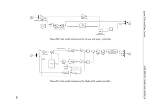


![Appendix C
Matlab: Scripts and figures
C.1 Simulation scripts
C.1.1 First set of simulation
1
2 %
3 % ∗ Matlab s c r i p t : 1 s t s e t of simulation . ∗
4 %
5 % Set up and run the Simulink model . This matlab s c r i p t corresponds to
6 % the f i r s t simulation , in which we aim to t e s t three values of each
7 % of the alphas keeping the order of magnitude of the o r i g i n a l value .
8 % In order to provide us enoough information , t h i s simulation i s
9 % s t r u c t u r e d in a way that f o r each alpha we t e s t a sm al le r and a
10 % bigger value than the o r i g i n a l .
11
12
13 c l e a r a l l ;
14 c l o s e a l l ;
15 c l c ;
16
17 %% D e f i n i t i o n of the parameters .
18
19 TMax = 6 0 0 ;
20 % Simulation time , 600 s or 10 min
21 alpha_1 = 0 . 1 ;
22 % O r i g i n a l value of the v a r i a b l e alpha 1 [−]
23 alpha_2 = 2 0 0 ;
24 % O r i g i n a l value of the v a r i a b l e alpha 2 [−]
25 alpha_3 = 1 ;
26 % O r i g i n a l value of the v a r i a b l e alpha 3 [−]
27 alpha_4 = 5 ;
28 % O r i g i n a l value of the v a r i a b l e alpha 4 [−]
29 i_min = 1 ;
30 i_max = 3 ;
31 % Set number of r e p e t i t i o n s
147](https://image.slidesharecdn.com/d5dea01b-1c58-4cb9-b6c8-8c7a99c48f71-161121112012/85/BACHELOR_THESIS_ACCELERATIOM-BASED_CONTROL_OF_OFFSHORE_WT-159-320.jpg)
![APPENDIX C. MATLAB: SCRIPTS AND FIGURES Ignasi Cifre and Àlex Garcia
32 counter = 0 ;
33
34
35 %% S e n i s t i v e a n a l y s i s of the f i r s t v a r i a b l e , alpha 1 , keeping the other
36 % v a r i a b l e s values as they were in the o r i g i n a l study . Also keeping the
37 % order of magnitude of the v a r i a b l e in the o r i g i n a l study .
38
39 alpha_1_min = 0 . 5 ;
40 % Set minimum alpha
41 alpha_1_max = 3 ;
42 % Set maximum alpha
43 alpha_1 = alpha_1_min ;
44 % Set alpha it ’ s being used
45 inc_alpha_1 = ( alpha_1_max−alpha_1_min ) / ( i_max−i_min ) ;
46 % Compute the required increment of the alpha .
47
48 f o r i = i_min : i_max ;
49 % Loop to t e s t values in alpha_1
50 FAST_InputFileName = ’ Test21 . fst ’ ;
51 % C a l l i n g t e s t 21
52 sim ( ’ STAFine . mdl ’ , [ 0 , TMax ] ) ;
53 % C a l l i n g Simulink
54 counter = counter + 1
55 f i n i s h =0;
56 % Set v a r i a b l e to check i f finished , to f a l s e
57 set_param ( ’ STAFine ’ , ’ SimulationCommand ’ , ’ Start ’ ) ;
58 % S t a r t s Simulink
59 while f i n i s h ==0
60 % Loop that f i n i s h e s once f i n i s h i s true
61 pause ( 6 0 0 ) ;
62 % Check each 10 minutes i f f i n i s h e d
63 s t a t e =get_param ( ’ STAFine ’ , ’ SimulationStatus ’ ) ;
64 % Get the s t a t e of the simulation
65 f i n i s h =strcmp ( state , ’ stopped ’ ) ;
66 % I f s t a t e g i v e s stopped , f i n i s h i s true
67 end
68
69 filename = s t r c a t ( ’ RB_a1_ ’ , num2str ( i ) ) ;
70 % Give a d i f f e r e n t name of f i l e f o r every i used
71 filename = s t r c a t ( filename , ’ . mat ’ ) ;
72 % Add . mat
73 save ( filename )
74 % Save the f i l e
75 alpha_1 = alpha_1 + inc_alpha_1 ;
76 % I n c r e a s e to next value of alpha
77 end
78
79 %% S e n i s t i v e a n a l y s i s of the second v a r i a b l e , alpha 2 , keeping the other
80 % v a r i a b l e s values as they were in the o r i g i n a l study . Also keeping the
81 % magnitude of the v a r i a b l e in the o r i g i n a l study .
82
83 alpha_1 = 0 . 1 ;
148](https://image.slidesharecdn.com/d5dea01b-1c58-4cb9-b6c8-8c7a99c48f71-161121112012/85/BACHELOR_THESIS_ACCELERATIOM-BASED_CONTROL_OF_OFFSHORE_WT-160-320.jpg)
![Ignasi Cifre and Àlex Garcia APPENDIX C. MATLAB: SCRIPTS AND FIGURES
84 %Reset alpha_1 to i t s i n i t i a l value .
85
86 % From that point , i t f o l l o w s e x a c t l y the
87 % same s t r u c t u r e as the f i r s t s e n s i t i v e a n a l y s i s .
88
89 alpha_2_min = 1 0 0 ;
90 alpha_2_max = 3 0 0 ;
91 alpha_2 = alpha_2_min ;
92 inc_alpha_2 = ( alpha_2_max−alpha_2_min ) / ( i_max−i_min ) ;
93
94 f o r i = i_min : i_max ;
95 FAST_InputFileName = ’ Test21 . fst ’ ;
96 sim ( ’ STAFine . mdl ’ , [ 0 , TMax ] ) ;
97 counter = counter + 1
98 f i n i s h =0;
99 set_param ( ’ STAFine ’ , ’ SimulationCommand ’ , ’ Start ’ ) ;
100 while f i n i s h ==0
101 pause ( 6 0 0 ) ;
102 s t a t e =get_param ( ’ STAFine ’ , ’ SimulationStatus ’ ) ;
103 f i n i s h =strcmp ( state , ’ stopped ’ ) ;
104 end
105 filename = s t r c a t ( ’ RB_a2_ ’ , num2str ( i ) ) ;
106 filename = s t r c a t ( filename , ’ . mat ’ ) ;
107 save ( filename )
108 alpha_2 = alpha_2 + inc_alpha_2 ;
109 end
110
111 %% S e n i s t i v e a n a l y s i s of the t h i r d v a r i a b l e , alpha 3 , keeping the other
112 % v a r i a b l e s values as they were in the o r i g i n a l study . Also keeping the
113 % magnitude of the v a r i a b l e in the o r i g i n a l study
114
115 alpha_2 = 200 ;
116
117 %Reset alpha_2 to i t s i n i t i a l value .
118
119 % From that point , i t f o l l o w s e x a c t l y the
120 % same s t r u c t u r e as the other s e n s i t i v e a n a l y s i s .
121
122 alpha_3_min = 0 . 0 1 ;
123 alpha_3_max = 5 ;
124 alpha_3 = alpha_3_min ;
125 inc_alpha_3 = ( alpha_3_max−alpha_3_min ) / ( i_max−i_min ) ;
126
127 f o r i = i_min : i_max ;
128 FAST_InputFileName = ’ Test21 . fst ’ ;
129 sim ( ’ STAFine . mdl ’ , [ 0 , TMax ] ) ;
130 counter = counter + 1
131 f i n i s h =0;
132 set_param ( ’ STAFine ’ , ’ SimulationCommand ’ , ’ Start ’ ) ;
133 while f i n i s h ==0
134 pause ( 6 0 0 ) ;
135 s t a t e =get_param ( ’ STAFine ’ , ’ SimulationStatus ’ ) ;
149](https://image.slidesharecdn.com/d5dea01b-1c58-4cb9-b6c8-8c7a99c48f71-161121112012/85/BACHELOR_THESIS_ACCELERATIOM-BASED_CONTROL_OF_OFFSHORE_WT-161-320.jpg)
![APPENDIX C. MATLAB: SCRIPTS AND FIGURES Ignasi Cifre and Àlex Garcia
136 f i n i s h =strcmp ( state , ’ stopped ’ ) ;
137 end
138 filename = s t r c a t ( ’ RB_a3_ ’ , num2str ( i ) ) ;
139 filename = s t r c a t ( filename , ’ . mat ’ ) ;
140 save ( filename )
141 alpha_3 = alpha_3 + inc_alpha_3 ;
142
143 end
144
145 %% S e n i s t i v e a n a l y s i s of the fourth v a r i a b l e , alpha 4 .
146
147 alpha_3 = 1 ;
148 %Reset alpha_2 to i t s i n i t i a l value .
149
150 % From that point , i t f o l l o w s e x a c t l y the
151 % same s t r u c t u r e as the other s e n s i t i v e a n a l y s i s .
152
153 alpha_4_min = 1 ;
154 alpha_4_max = 2 0 ;
155 alpha_4 = alpha_4_min ;
156 inc_alpha_4 = ( alpha_4_max−alpha_4_min ) / ( i_max−i_min ) ;
157
158 f o r i = i_min : i_max ;
159 FAST_InputFileName = ’ Test21 . fst ’ ;
160 sim ( ’ STAFine . mdl ’ , [ 0 , TMax ] ) ;
161 counter = counter + 1
162 f i n i s h =0;
163 set_param ( ’ STAFine ’ , ’ SimulationCommand ’ , ’ Start ’ ) ;
164 while f i n i s h ==0
165 pause ( 6 0 0 ) ;
166 s t a t e =get_param ( ’ STAFine ’ , ’ SimulationStatus ’ ) ;
167 f i n i s h =strcmp ( state , ’ stopped ’ ) ;
168 end
169 filename = s t r c a t ( ’ RB_a4_ ’ , num2str ( i ) ) ;
170 filename = s t r c a t ( filename , ’ . mat ’ ) ;
171 save ( filename )
172 alpha_4 = alpha_4 + inc_alpha_4 ;
173
174 end
C.1.2 Second set of simulation
1
2 %
3 % ∗ Matlab s c r i p t : 2nd s e t of s i m u l a t i o n . ∗
4 %
5 % Set up and run the Simulink model . This matlab s c r i p t c o r r e s p o n d s to
6 % the second simulation , in which we aim to t e s t a v a l u e f o r each alpha
7 % changing the order of magnitude .
8
150](https://image.slidesharecdn.com/d5dea01b-1c58-4cb9-b6c8-8c7a99c48f71-161121112012/85/BACHELOR_THESIS_ACCELERATIOM-BASED_CONTROL_OF_OFFSHORE_WT-162-320.jpg)
![Ignasi Cifre and Àlex Garcia APPENDIX C. MATLAB: SCRIPTS AND FIGURES
9 clear a l l ;
10 close a l l ;
11 clc ;
12
13 %% D e f i n i t i o n of the parameters .
14
15 TMax = 6 0 0 ;
16 % S i m u l a t i o n time , 600 s or 10 min
17 alpha_1 = 0 . 1 ;
18 % O r i g i n a l v a l u e of the v a r i a b l e alpha 1 [−]
19 alpha_2 = 2 0 0 ;
20 % O r i g i n a l v a l u e of the v a r i a b l e alpha 2 [−]
21 alpha_3 = 1 ;
22 % O r i g i n a l v a l u e of the v a r i a b l e alpha 3 [−]
23 alpha_4 = 5 ;
24 % O r i g i n a l v a l u e of the v a r i a b l e alpha 4 [−]
25 counter = 0 ;
26
27
28 %% A n a l y s i s of the f i r s t v a r i a b l e , alpha 1 , keeping the o t h e r
29 % v a r i a b l e s v a l u e s as they were in the o r i g i n a l study .
30
31 alpha_1 = 2 0 ;
32 % Set alpha 1 to 20 to t e s t i t .
33
34 FAST_InputFileName = ’ Test21 . f s t ’ ;
35 % C a l l i n g t e s t 21
36 sim ( ’STAFine_CONTROL . mdl ’ , [ 0 , TMax ] ) ;
37 % C a l l i n g Simulink model
38 counter = counter + 1
39 f i n i s h =0;
40 % Set v a r i a b l e to check i f f i n i s h e d , to f a l s e
41 set_param ( ’STAFine_CONTROL ’ , ’ SimulationCommand ’ , ’ S t a r t ’ ) ;
42 % S t a r t s Simulink
43 while f i n i s h ==0
44 % Loop t h a t f i n i s h e s once f i n i s h i s t r u e
45 pause ( 6 0 0 ) ;
46 % Check each 10 minutes i f f i n i s h e d
47 s t a t e =get_param ( ’STAFine_CONTROL ’ , ’ SimulationStatus ’ ) ;
48 % Get the s t a t e of the s i m u l a t i o n
49 f i n i s h =strcmp ( state , ’ stopped ’ ) ;
50 % I f s t a t e g i v e s stopped , f i n i s h i s t r u e
51 end
52
53 filename = s t r c a t ( ’ R2_a1 ’ ) ;
54 % Give a d i f f e r e n t name of f i l e f o r every i used
55 filename = s t r c a t ( filename , ’ . mat ’ ) ;
56 % Add . mat
57 save ( filename )
58 % Save the f i l e
59
60
151](https://image.slidesharecdn.com/d5dea01b-1c58-4cb9-b6c8-8c7a99c48f71-161121112012/85/BACHELOR_THESIS_ACCELERATIOM-BASED_CONTROL_OF_OFFSHORE_WT-163-320.jpg)
![APPENDIX C. MATLAB: SCRIPTS AND FIGURES Ignasi Cifre and Àlex Garcia
61 %% A n a l y s i s of the second v a r i a b l e , alpha 2 , keeping the o t h e r
62 % v a r i a b l e s v a l u e s as they were in the o r i g i n a l study .
63
64 alpha_1 = 0 . 1 ;
65 % Set alpha 1 to i t s i n i t i a l v a l u e .
66 alpha_2 = 1 0 0 0 ;
67 % Set alpha 2 to 1000 to t e s t i t .
68
69 FAST_InputFileName = ’ Test21 . f s t ’ ;
70 % C a l l i n g t e s t 21
71 sim ( ’STAFine_CONTROL . mdl ’ , [ 0 , TMax ] ) ;
72 % C a l l i n g Simulink
73 counter = counter + 1
74 f i n i s h =0;
75 % Set v a r i a b l e to check i f f i n i s h e d , to f a l s e
76 set_param ( ’STAFine_CONTROL ’ , ’ SimulationCommand ’ , ’ S t a r t ’ ) ;
77 % S t a r t s Simulink
78 while f i n i s h ==0
79 % Loop t h a t f i n i s h e s once f i n i s h i s t r u e
80 pause ( 6 0 0 ) ;
81 % Check each 10 minutes i f f i n i s h e d
82 s t a t e =get_param ( ’STAFine_CONTROL ’ , ’ SimulationStatus ’ ) ;
83 % Get the s t a t e of the s i m u l a t i o n
84 f i n i s h =strcmp ( state , ’ stopped ’ ) ;
85 % I f s t a t e g i v e s stopped , f i n i s h i s t r u e
86 end
87 filename = s t r c a t ( ’ R2_a2 ’ ) ;
88 % Give a d i f f e r e n t name of f i l e f o r every i used
89 filename = s t r c a t ( filename , ’ . mat ’ ) ;
90 % Add . mat
91 save ( filename )
92 % Save the f i l e
93
94
95 %% A n a l y s i s of the t h i r d v a r i a b l e , alpha 3 , keeping the o t h e r
96 % v a r i a b l e s v a l u e s as they were in the o r i g i n a l study .
97
98 alpha_2 = 2 0 0 ;
99 % Set alpha 2 to i t s i n i t i a l v a l u e .
100 alpha_3 = 2 0 ;
101 % Set alpha 3 to 20 to t e s t i t .
102
103
104 FAST_InputFileName = ’ Test21 . f s t ’ ;
105 % C a l l i n g t e s t 21
106 sim ( ’STAFine_CONTROL . mdl ’ , [ 0 , TMax ] ) ;
107 % C a l l i n g Simulink
108 counter = counter + 1
109 f i n i s h =0;
110 % Set v a r i a b l e to check i f f i n i s h e d , to f a l s e
111 set_param ( ’STAFine_CONTROL ’ , ’ SimulationCommand ’ , ’ S t a r t ’ ) ;
112 % S t a r t s Simulink
152](https://image.slidesharecdn.com/d5dea01b-1c58-4cb9-b6c8-8c7a99c48f71-161121112012/85/BACHELOR_THESIS_ACCELERATIOM-BASED_CONTROL_OF_OFFSHORE_WT-164-320.jpg)
![Ignasi Cifre and Àlex Garcia APPENDIX C. MATLAB: SCRIPTS AND FIGURES
113 while f i n i s h ==0
114 % Loop t h a t f i n i s h e s once f i n i s h i s t r u e
115 pause ( 6 0 0 ) ;
116 % Check each 10 minutes i f the s i m u l a t i o n has f i n i s h e d
117 s t a t e =get_param ( ’STAFine_CONTROL ’ , ’ SimulationStatus ’ ) ;
118 % Get the s t a t e of the s i m u l a t i o n
119 f i n i s h =strcmp ( state , ’ stopped ’ ) ;
120 % I f s t a t e g i v e s stopped , f i n i s h i s t r u e
121 end
122 filename = s t r c a t ( ’ R2_a3 ’ ) ;
123 % Give a d i f f e r e n t name of f i l e f o r every i used
124 filename = s t r c a t ( filename , ’ . mat ’ ) ;
125 % Add . mat
126 save ( filename )
127 % Save the f i l e
128
129
130
131 %% S e n i s t i v e a n a l y s i s of the f o u r t h v a r i a b l e , alpha 4 , keeping the o t h e r
132 % v a r i a b l e s v a l u e s as they were in the o r i g i n a l study .
133
134 alpha_3 = 1 ;
135 % Set alpha 3 to i t s i n i t i a l v a l u e .
136 alpha_4 = 5 0 ;
137 % Set alpha 4 to 50 to t e s t i t .
138
139 FAST_InputFileName = ’ Test21 . f s t ’ ;
140 % C a l l i n g t e s t 21
141 sim ( ’STAFine_CONTROL . mdl ’ , [ 0 , TMax ] ) ;
142 % C a l l i n g Simulink
143 counter = counter + 1
144 f i n i s h =0;
145 % Set v a r i a b l e to check i f f i n i s h e d , to f a l s e
146 set_param ( ’STAFine_CONTROL ’ , ’ SimulationCommand ’ , ’ S t a r t ’ ) ;
147 % S t a r t s Simulink
148 while f i n i s h ==0
149 % Loop t h a t f i n i s h e s once f i n i s h i s t r u e
150 pause ( 6 0 0 ) ;
151 % Check each 10 minutes i f f i n i s h e d
152 s t a t e =get_param ( ’STAFine_CONTROL ’ , ’ SimulationStatus ’ ) ;
153 % Get the s t a t e of the s i m u l a t i o n
154 f i n i s h =strcmp ( state , ’ stopped ’ ) ;
155 % I f s t a t e g i v e s stopped , f i n i s h i s t r u e
156 end
157 filename = s t r c a t ( ’ R2_a4 ’ ) ;
158 % Give a d i f f e r e n t name of f i l e f o r every i used
159 filename = s t r c a t ( filename , ’ . mat ’ ) ;
160 % Add . mat
161 save ( filename )
162 % Save the f i l e
153](https://image.slidesharecdn.com/d5dea01b-1c58-4cb9-b6c8-8c7a99c48f71-161121112012/85/BACHELOR_THESIS_ACCELERATIOM-BASED_CONTROL_OF_OFFSHORE_WT-165-320.jpg)
![APPENDIX C. MATLAB: SCRIPTS AND FIGURES Ignasi Cifre and Àlex Garcia
C.1.3 Third set of simulation
1
2 %
3 % ∗ Matlab s c r i p t : 3 rd s e t of s i m u l a t i o n . ∗
4 %
5 % Set up and run the Simulink model . This matlab s c r i p t c o r r e s p o n d s to
6 % the t h i r d simulation , in which we aim to t e s t four d i f f e r e n t s v a l u e s
7 % f o r alpha 2 , changing each time the magnitude order of the v a l u e .
8
9
10 clear a l l ;
11 close a l l ;
12 clc ;
13
14 %% D e f i n i t i o n of the parameters .
15
16 TMax = 6 0 0 ;
17 % S i m u l a t i o n time , 600 s or 10 min
18 alpha_1 = 0 . 1 ;
19 % O r i g i n a l v a l u e of the v a r i a b l e alpha 1 [−]
20 alpha_3 = 1 ;
21 % O r i g i n a l v a l u e of the v a r i a b l e alpha 3 [−]
22 alpha_4 = 5 ;
23 % O r i g i n a l v a l u e of the v a r i a b l e alpha 4 [−]
24 counter = 0 ;
25
26 %% F i r s t t e s t : alpha_2 = 0 . 0 1 .
27
28 alpha_2 = 0 . 0 1 ;
29 % Set the v a l u e of alpha_2
30
31 FAST_InputFileName = ’ Test21 . f s t ’ ;
32 % C a l l i n g t e s t 21
33 sim ( ’STAFine_CONTROL . mdl ’ , [ 0 , TMax ] ) ;
34 % C a l l i n g Simulink
35 counter = counter + 1
36 f i n i s h =0;
37 % Set v a r i a b l e to check i f f i n i s h e d , to f a l s e
38 set_param ( ’STAFine_CONTROL ’ , ’ SimulationCommand ’ , ’ S t a r t ’ ) ;
39 % S t a r t s Simulink
40 while f i n i s h ==0
41 % Loop t h a t f i n i s h e s once f i n i s h i s t r u e
42 pause ( 6 0 0 ) ;
43 % Check each 10 minutes i f f i n i s h e d
44 s t a t e =get_param ( ’STAFine_CONTROL ’ , ’ SimulationStatus ’ ) ;
45 % Get the s t a t e of the s i m u l a t i o n
46 f i n i s h =strcmp ( state , ’ stopped ’ ) ;
47 % I f s t a t e g i v e s stopped , f i n i s h i s t r u e
48 end
49
50 filename = s t r c a t ( ’ R3_a2_1 ’ ) ;
154](https://image.slidesharecdn.com/d5dea01b-1c58-4cb9-b6c8-8c7a99c48f71-161121112012/85/BACHELOR_THESIS_ACCELERATIOM-BASED_CONTROL_OF_OFFSHORE_WT-166-320.jpg)
![Ignasi Cifre and Àlex Garcia APPENDIX C. MATLAB: SCRIPTS AND FIGURES
51 % Give a name f o r the f i l e .
52 filename = s t r c a t ( filename , ’ . mat ’ ) ;
53 % Add . mat
54 save ( filename )
55
56 %% Second t e s t t e s t : alpha_2 = 1 0 0 0 0 .
57
58 % I t f o l l o w s the same s t e p s as in the f i r s t t e s t of t h i s s c r i p t .
59
60 alpha_2 = 1 0 0 00 ;
61
62
63 FAST_InputFileName = ’ Test21 . f s t ’ ;
64 sim ( ’STAFine_CONTROL . mdl ’ , [ 0 , TMax ] ) ;
65 counter = counter + 1
66 f i n i s h =0;
67 set_param ( ’STAFine_CONTROL ’ , ’ SimulationCommand ’ , ’ S t a r t ’ ) ;
68 while f i n i s h ==0
69 pause ( 6 0 0 ) ;
70 s t a t e =get_param ( ’STAFine_CONTROL ’ , ’ SimulationStatus ’ ) ;
71 f i n i s h =strcmp ( state , ’ stopped ’ ) ;
72 end
73
74 filename = s t r c a t ( ’ R3_a2_2 ’ ) ;
75 filename = s t r c a t ( filename , ’ . mat ’ ) ;
76 save ( filename )
77
78 %% Third t e s t t e s t : alpha_2 = 1 0 0 0 0 0 .
79
80 % I t f o l l o w s the same s t e p s as in the f i r s t t e s t of t h i s s c r i p t .
81
82 alpha_2 = 100000;
83
84 FAST_InputFileName = ’ Test21 . f s t ’ ;
85 sim ( ’STAFine_CONTROL . mdl ’ , [ 0 , TMax ] ) ;
86 counter = counter + 1
87 f i n i s h =0;
88 set_param ( ’STAFine_CONTROL ’ , ’ SimulationCommand ’ , ’ S t a r t ’ ) ;
89 while f i n i s h ==0
90 pause ( 6 0 0 ) ;
91 s t a t e =get_param ( ’STAFine_CONTROL ’ , ’ SimulationStatus ’ ) ;
92 f i n i s h =strcmp ( state , ’ stopped ’ ) ;
93 end
94 filename = s t r c a t ( ’ R3_a2_3 ’ ) ;
95 filename = s t r c a t ( filename , ’ . mat ’ ) ;
96 save ( filename )
97
98
99 %% Fourth t e s t : alpha_2 = 1 0 0 0 0 0 0 .
100
101 % I t f o l l o w s the same s t e p s as in the f i r s t t e s t of t h i s s c r i p t .
102
155](https://image.slidesharecdn.com/d5dea01b-1c58-4cb9-b6c8-8c7a99c48f71-161121112012/85/BACHELOR_THESIS_ACCELERATIOM-BASED_CONTROL_OF_OFFSHORE_WT-167-320.jpg)
![APPENDIX C. MATLAB: SCRIPTS AND FIGURES Ignasi Cifre and Àlex Garcia
103 alpha_2 = 1000000 ;
104
105 FAST_InputFileName = ’ Test21 . f s t ’ ;
106 sim ( ’STAFine_CONTROL . mdl ’ , [ 0 , TMax ] ) ;
107 counter = counter + 1
108 f i n i s h =0;
109 set_param ( ’STAFine_CONTROL ’ , ’ SimulationCommand ’ , ’ S t a r t ’ ) ;
110 while f i n i s h ==0
111 pause ( 6 0 0 ) ;
112 s t a t e =get_param ( ’STAFine_CONTROL ’ , ’ SimulationStatus ’ ) ;
113 f i n i s h =strcmp ( state , ’ stopped ’ ) ;
114 end
115 filename = s t r c a t ( ’ R3_a2_4 ’ ) ;
116 filename = s t r c a t ( filename , ’ . mat ’ ) ;
117 save ( filename )
C.1.4 Fourth set of simulation
1
2 %
3 % ∗ Matlab s c r i p t : 4 th s e t of s i m u l a t i o n . ∗
4 %
5 % Set up and run the Simulink model . This matlab s c r i p t c o r r e s p o n d s to
6 % the f o u r t h simulation , in which we aim to t e s t some combinations of
7 % alpha 2 and alpha 4 . Each of the alphas i s t e s t e s betweeen a
8 % d e s i r e d range . This range i s d e f i n e d with the i n f o r m a t i o n obtained
9 % from p r e v i o u s s i m u l a t i o n s .
10
11
12 clear a l l ;
13 close a l l ;
14 clc ;
15
16 %% D e f i n i t i o n of the parameters .
17
18 TMax = 6 0 0 ;
19 % S i m u l a t i o n time , 600 s or 10 min
20 alpha_1 = 0 . 1 ;
21 % O r i g i n a l v a l u e of the v a r i a b l e alpha 1 [−]
22 alpha_3 = 1 ;
23 % O r i g i n a l v a l u e of the v a r i a b l e alpha 3 [−]
24
25 i_min = 1 ;
26 i_max = 4 ;
27 % Set number of r e p e t i t i o n s of alpha 2
28 j_min = 1 ;
29 j_max = 4 ;
30 % Set number of r e p e t i t i o n s of alpha 4
31 counter = 0 ;
32
156](https://image.slidesharecdn.com/d5dea01b-1c58-4cb9-b6c8-8c7a99c48f71-161121112012/85/BACHELOR_THESIS_ACCELERATIOM-BASED_CONTROL_OF_OFFSHORE_WT-168-320.jpg)
![Ignasi Cifre and Àlex Garcia APPENDIX C. MATLAB: SCRIPTS AND FIGURES
33
34 %% S e n s i t i v e a n a l y s i s of both alpha 2 and alpha 4 . We d e f i n e a double loop
35 % in which we make combinations of some v a l u e s of the parameters .
36
37
38
39 alpha_2_min = 7 5 0 ;
40 % Set minimum alpha 2
41 alpha_2_max = 1 2 5 0 ;
42 % Set maximum alpha 2
43 alpha_2 = alpha_2_min ;
44 % Set alpha 2 t h a t i s used at the b e g i n n i n g
45 inc_alpha_2 = ( alpha_2_max−alpha_2_min ) / ( i_max−i_min ) ;
46 % Compute the r e q u i r e d increment
47
48 for i = i_min : i_max ;
49 % Loop to t e s t v a l u e s in alpha_2
50 alpha_4_min = 5 ;
51 % Set minimum alpha 4
52 alpha_4_max = 5 0 ;
53 % Set maximum alpha 4
54 alpha_4 = alpha_4_min ;
55 % Set alpha 4 t h a t i s used at the b e g i n n i n g
56 inc_alpha_4 = ( alpha_4_max−alpha_4_min ) / ( j_max−j_min ) ;
57 % Compute the r e q u i r e d increment
58 for j = j_min : j_max ;
59 % Loop to t e s t v a l u e s in alpha_2
60 FAST_InputFileName = ’ Test21 . f s t ’ ;
61 % C a l l i n g t e s t 21
62 sim ( ’STAFine_CONTROL . mdl ’ , [ 0 , TMax ] ) ;
63 % C a l l i n g Simulink
64 counter = counter + 1
65 f i n i s h =0;
66 % Set v a r i a b l e to check i f f i n i s h e d , to f a l s e
67 set_param ( ’STAFine_CONTROL ’ , ’ SimulationCommand ’ , ’ S t a r t ’ ) ;
68 % S t a r t s Simulink
69 while f i n i s h ==0
70 % Loop t h a t f i n i s h e s once f i n i s h i s t r u e
71 pause ( 6 0 0 ) ;
72 % Check each 10 seconds i f f i n i s h e d
73 s t a t e =get_param ( ’STAFine_CONTROL ’ , ’ SimulationStatus ’ ) ;
74 % Get the s t a t e of the s i m u l a t i o n
75 f i n i s h =strcmp ( state , ’ stopped ’ ) ;
76 % I f s t a t e g i v e s stopped , f i n i s h i s t r u e
77 end
78
79 filename = s t r c a t ( ’ R4_ ’ , num2str ( i ) , num2str ( j ) ) ;
80 % Give a d i f f e r e n t name of f i l e f o r every i used
81 filename = s t r c a t ( filename , ’ . mat ’ ) ;
82 % Add . mat
83 save ( filename )
84 % Save the f i l e
157](https://image.slidesharecdn.com/d5dea01b-1c58-4cb9-b6c8-8c7a99c48f71-161121112012/85/BACHELOR_THESIS_ACCELERATIOM-BASED_CONTROL_OF_OFFSHORE_WT-169-320.jpg)
![APPENDIX C. MATLAB: SCRIPTS AND FIGURES Ignasi Cifre and Àlex Garcia
85 alpha_4 = alpha_4 + inc_alpha_4 ;
86 % I n c r e a s e to next v a l u e of alpha 4
87 end
88 alpha_2 = alpha_2 + inc_alpha_2 ;
89 % I n c r e a s e to next v a l u e of alpha 4
90 end
C.1.5 Fifth set of simulation
1
2 %
3 % ∗ Matlab s c r i p t : 5 th s e t of s i m u l a t i o n . ∗
4 %
5 % Set up and run the Simulink model . This matlab s c r i p t c o r r e s p o n d s to
6 % the f i f t h simulation , in which we aim to t e s t t h r e e v a l u e s of alpha 1
7 % to t r y to a c c u r a t e the o p e r a t i n g range of t h i s parameter .
8
9 clear a l l ;
10 close a l l ;
11 clc ;
12
13
14 TMax = 6 0 0 ;
15 % S i m u l a t i o n time , 600 s or 10 min
16 alpha_2 = 1 2 5 0 ;
17 % O r i g i n a l v a l u e of the v a r i a b l e alpha 1 [−]
18 alpha_3 = 1 ;
19 % O r i g i n a l v a l u e of the v a r i a b l e alpha 3 [−]
20 alpha_4 = 5 ;
21 % O r i g i n a l v a l u e of the v a r i a b l e alpha 4 [−]
22 i_min = 1 ;
23 i_max = 3 ;
24 % Set number of r e p e t i t i o n s
25 counter = 0 ;
26
27
28 %% S e n i s t i v e a n a l y s i s of alpha 1 , keeping the o t h e r
29 % v a r i a b l e s v a l u e s as they were in the o r i g i n a l study .
30
31 alpha_1_min = 1 ;
32 % Set minimum alpha
33 alpha_1_max = 1 0 ;
34 % Set maximum alpha
35 alpha_1 = alpha_1_min ;
36 % Set alpha i t ’ s being used
37 inc_alpha_1 = ( alpha_1_max−alpha_1_min ) / ( i_max−i_min ) ;
38 % Compute the r e q u i r e d increment
39 for i = i_min : i_max ;
40 % Loop to t e s t v a l u e s in alpha_1
41 FAST_InputFileName = ’ Test21 . f s t ’ ;
158](https://image.slidesharecdn.com/d5dea01b-1c58-4cb9-b6c8-8c7a99c48f71-161121112012/85/BACHELOR_THESIS_ACCELERATIOM-BASED_CONTROL_OF_OFFSHORE_WT-170-320.jpg)
![Ignasi Cifre and Àlex Garcia APPENDIX C. MATLAB: SCRIPTS AND FIGURES
42 % C a l l i n g t e s t 21
43 sim ( ’STAFine_CONTROL . mdl ’ , [ 0 , TMax ] ) ;
44 % C a l l i n g Simulink
45 counter = counter + 1
46 f i n i s h =0;
47 % Set v a r i a b l e to check i f f i n i s h e d , to f a l s e
48 set_param ( ’STAFine_CONTROL ’ , ’ SimulationCommand ’ , ’ S t a r t ’ ) ;
49 % S t a r t s Simulink
50 while f i n i s h ==0
51 % Loop t h a t f i n i s h e s once f i n i s h i s t r u e
52 pause ( 6 0 0 ) ;
53 % Check each 10 minutes i f f i n i s h e d
54 s t a t e =get_param ( ’STAFine_CONTROL ’ , ’ SimulationStatus ’ ) ;
55 % Get the s t a t e of the s i m u l a t i o n
56 f i n i s h =strcmp ( state , ’ stopped ’ ) ;
57 % I f s t a t e g i v e s stopped , f i n i s h i s t r u e
58 end
59
60 filename = s t r c a t ( ’ R5_a1_ ’ , num2str ( i ) ) ;
61 % Give a d i f f e r e n t name of f i l e f o r every i used
62 filename = s t r c a t ( filename , ’ . mat ’ ) ;
63 % Add . mat
64 save ( filename )
65 % Save the f i l e
66 alpha_1 = alpha_1 + inc_alpha_1 ;
67 % I n c r e a s e to next v a l u e of alpha 1
68 end
159](https://image.slidesharecdn.com/d5dea01b-1c58-4cb9-b6c8-8c7a99c48f71-161121112012/85/BACHELOR_THESIS_ACCELERATIOM-BASED_CONTROL_OF_OFFSHORE_WT-171-320.jpg)