This document is a thesis submitted by Mark Kenneth Quinn to the University of Manchester for the degree of Doctor of Philosophy. It investigates shock diffraction phenomena and their measurement through a combination of experimental and numerical techniques. The thesis contains literature on shock waves, shock tubes, shock diffraction, shear layers, and numerical simulations. It then describes the experimental techniques of schlieren, particle image velocimetry (PIV), pressure measurements, and pressure-sensitive paint (PSP) used to study the phenomena. The apparatus and simulation setup are also outlined. Results are then presented and discussed for shock diffraction around sharp and round geometries based on density and particle-based measurements for a range of Mach numbers.


![List of Figures
2.1 Schematic of shockwave frame of reference . . . . . . . . . . . . . . . 6
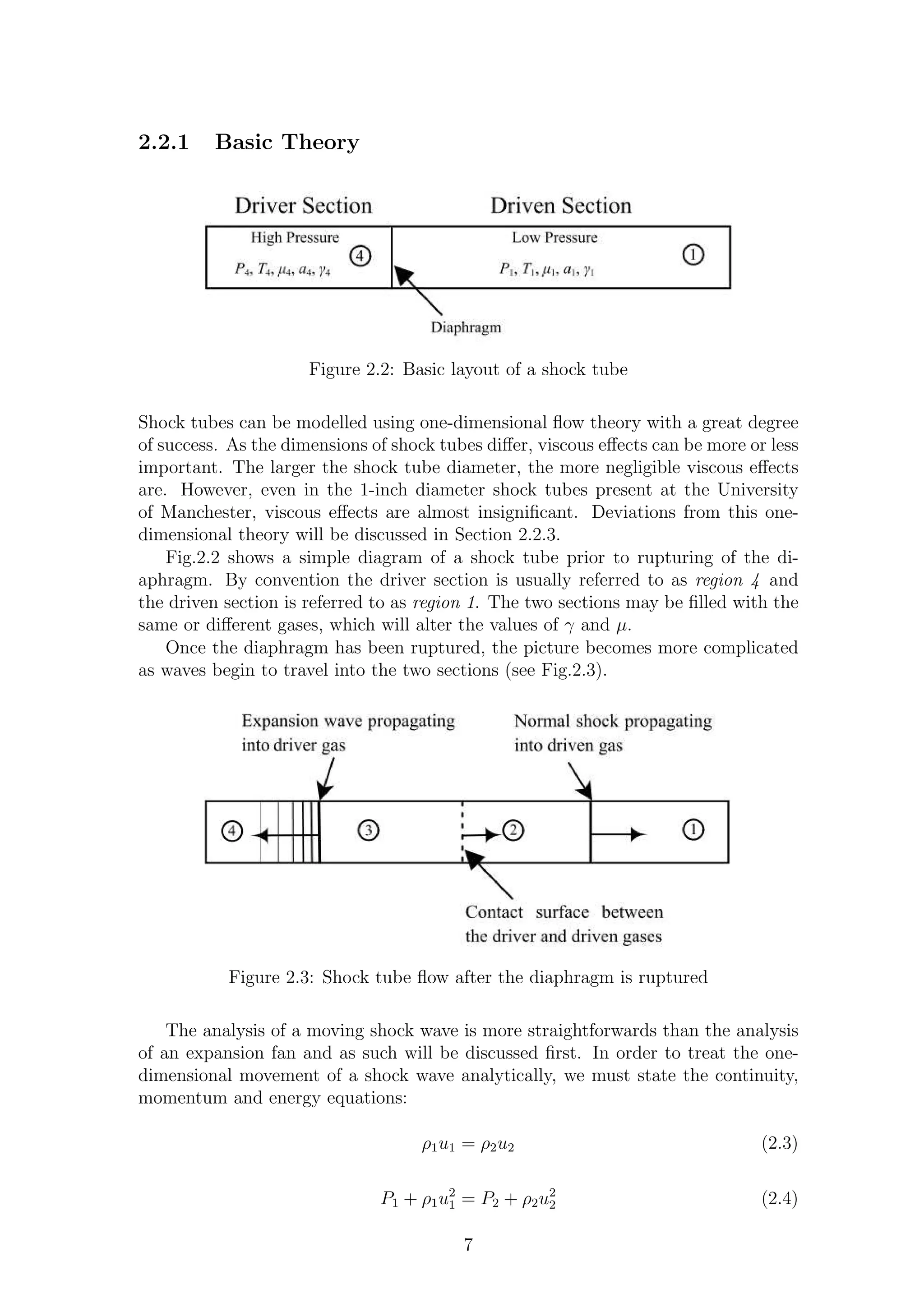
2.2 Basic layout of a shock tube . . . . . . . . . . . . . . . . . . . . . . . 7
2.3 Shock tube flow after the diaphragm is ruptured . . . . . . . . . . . . 7
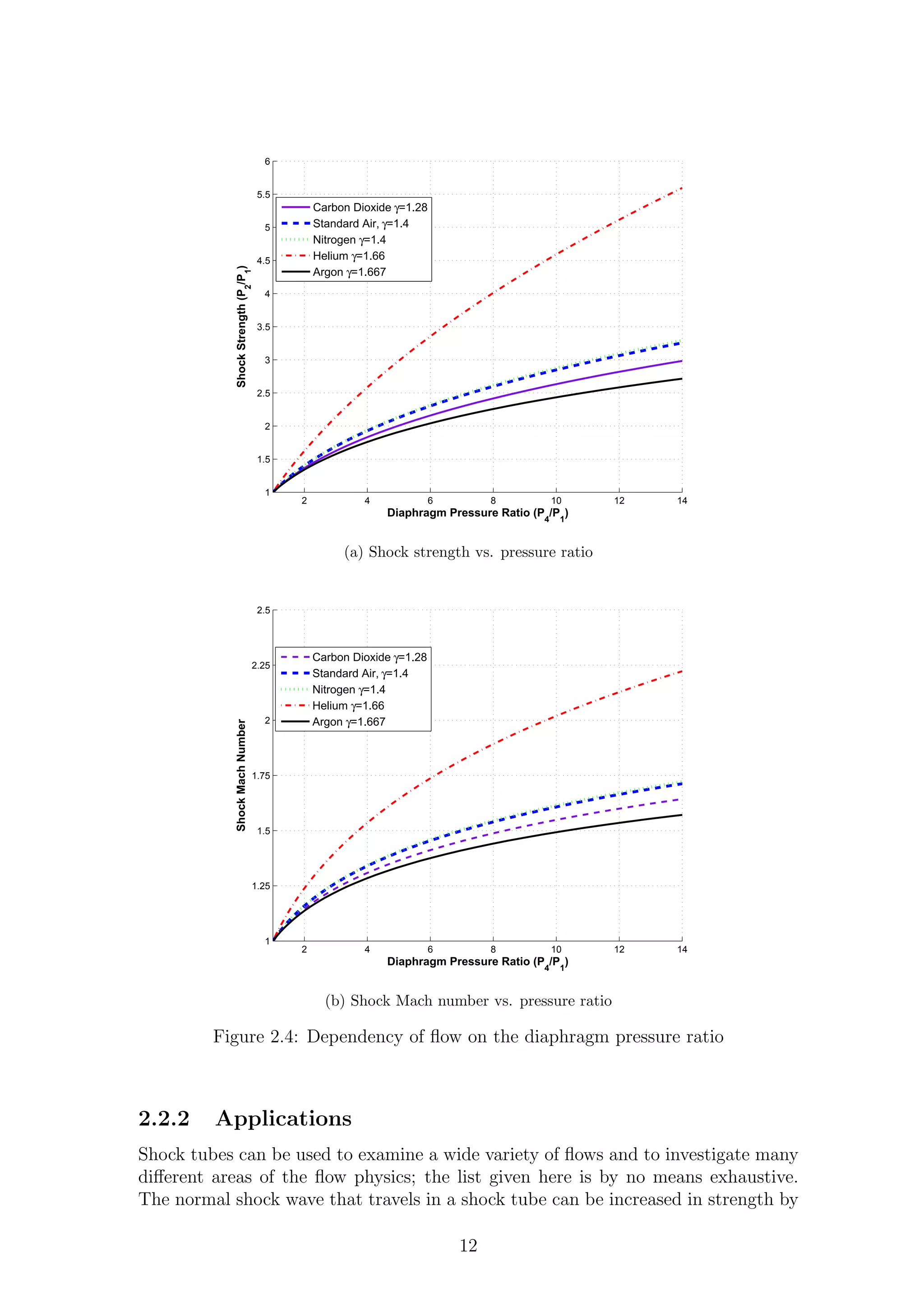
2.4 Dependency of flow on the diaphragm pressure ratio . . . . . . . . . . 12
2.4 Dependency of flow on the diaphragm pressure ratio . . . . . . . . . . 13
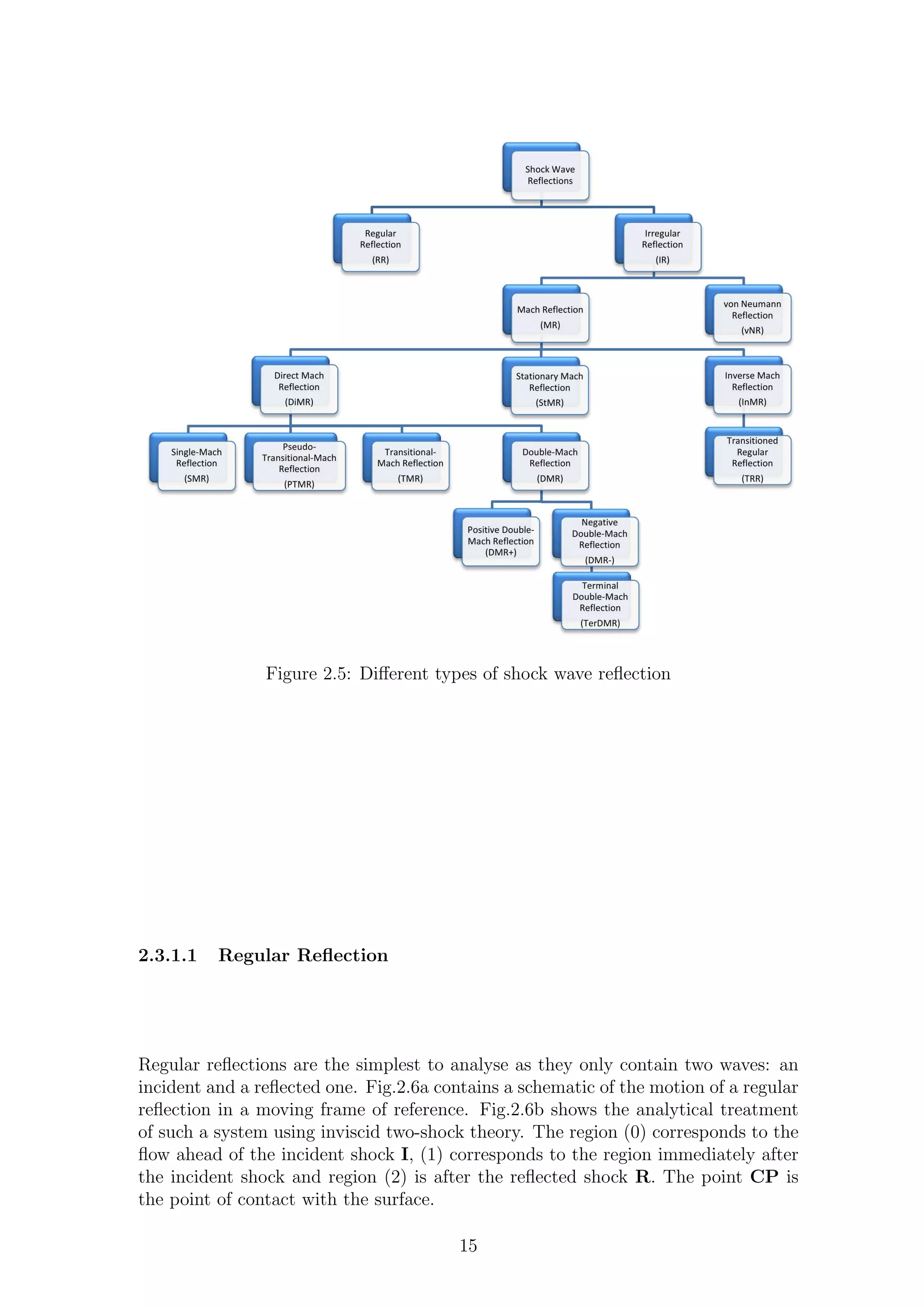
2.5 Different types of shock wave reflection . . . . . . . . . . . . . . . . . 15
2.6 Analysis of regular reflection: (a) lab frame of reference and (b) show-
ing two-shock theory . . . . . . . . . . . . . . . . . . . . . . . . . . . 16
2.7 Shock polar with θw = 9◦
and M0 = 2 . . . . . . . . . . . . . . . . . . 17
2.8 Analysis of a pseudo-steady Mach reflection . . . . . . . . . . . . . . 18
2.10 Position of curved shocks and rays . . . . . . . . . . . . . . . . . . . . 18
2.9 Shock polar with θw = 19◦
and M0 = 2.5 . . . . . . . . . . . . . . . . 19
2.11 Shock front profile after a sharp corner . . . . . . . . . . . . . . . . . 20
2.12 Basic flow structure behind a shock wave diffracting around a sharp
corner . . . . . . . . . . . . . . . . . . . . . . . . . . . . . . . . . . . 21
2.13 Close-up of the expansion wave . . . . . . . . . . . . . . . . . . . . . 22
2.14 Flow structure created by a rounded corner . . . . . . . . . . . . . . 24
2.15 Kelvin-Helmholtz instability images on Saturn taken by the Cassini
Orbiter . . . . . . . . . . . . . . . . . . . . . . . . . . . . . . . . . . 26
2.16 Schematic of the flow showing a discontinuity in the velocity profile
and the assumed disturbance . . . . . . . . . . . . . . . . . . . . . . . 26
2.17 Stability contour as calculated by Miles [1] . . . . . . . . . . . . . . . 30
2.18 Starting vortices generated by Pullin & Perry [2] . . . . . . . . . . . . 32
2.19 Planar shock I impacting on vortex V . . . . . . . . . . . . . . . . . 34
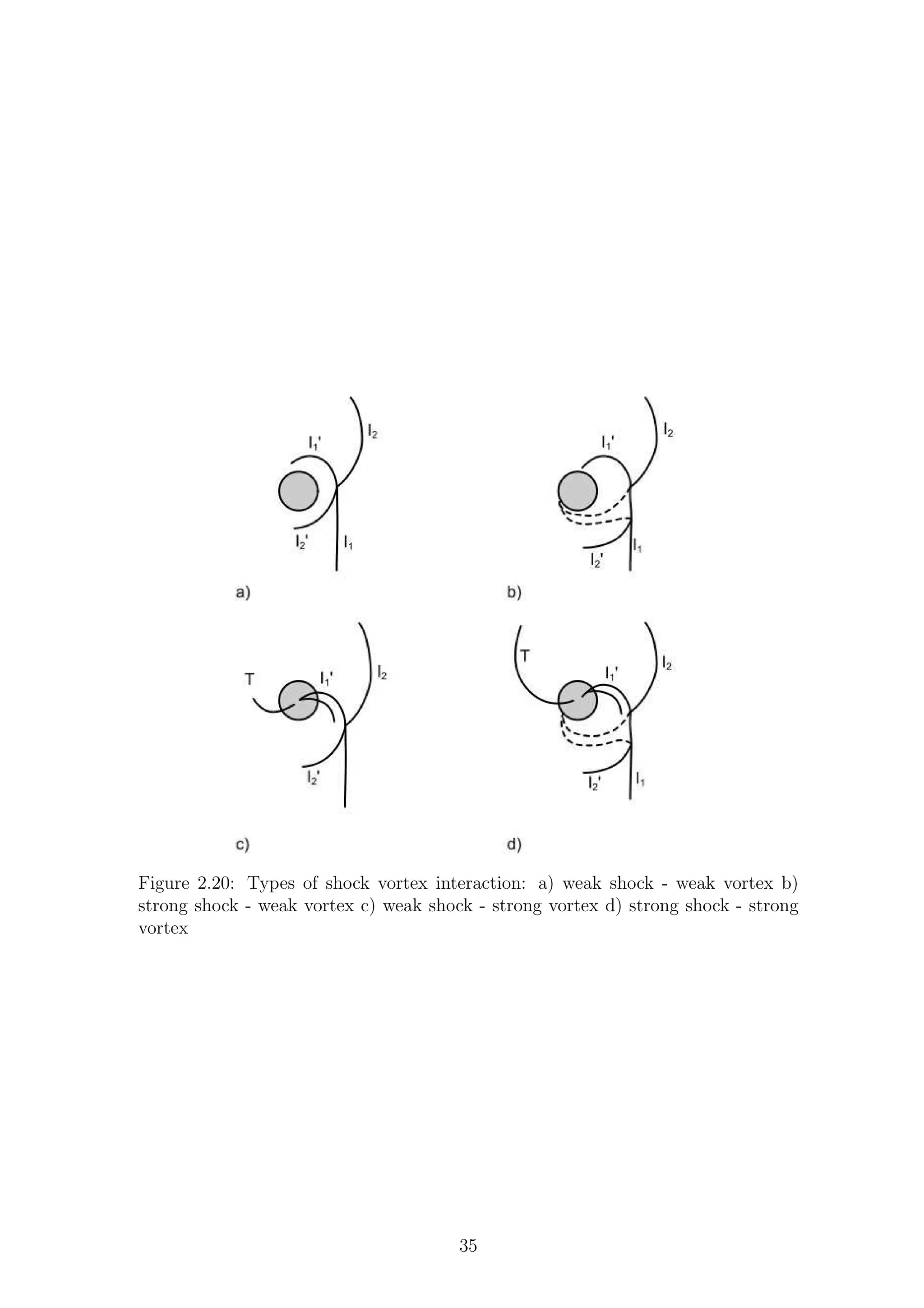
2.20 Types of shock vortex interaction: a) weak shock - weak vortex b)
strong shock - weak vortex c) weak shock - strong vortex d) strong
shock - strong vortex . . . . . . . . . . . . . . . . . . . . . . . . . . . 35
3.1 Original sketches of shadowgraphs seen by Marat [3] . . . . . . . . . . 45
3.2 Diagram of refraction of light through a change in refractive index . . 47
3.3 Principle of shadowgraphy . . . . . . . . . . . . . . . . . . . . . . . . 48
3.4 Homemade shadowgraph of a lighter flame . . . . . . . . . . . . . . . 49
3.5 Principle of focused shadowgraphy . . . . . . . . . . . . . . . . . . . 49
3.6 Principle of schieren imaging . . . . . . . . . . . . . . . . . . . . . . . 50
3.7 Diagram of knife-edge plane . . . . . . . . . . . . . . . . . . . . . . . 50
3.8 x-t diagram for a Mi = 1.46 shock . . . . . . . . . . . . . . . . . . . . 52
3.9 Schlieren setup . . . . . . . . . . . . . . . . . . . . . . . . . . . . . . 53
3.10 Depth of field of a shadowgraph system . . . . . . . . . . . . . . . . . 54
3.11 Field of view of the schlieren system (all dimensions in mm) . . . . . 55
ix](https://image.slidesharecdn.com/4a6f74b5-6bbb-4ffd-b3f5-7486cdb057cd-150303082443-conversion-gate01/75/Mark-Quinn-Thesis-10-2048.jpg)
![3.12 Two identical shadowgraph images before and after processing . . . . 56
3.13 Experimental vs. theoretical incident shock Mach number . . . . . . 57
3.14 Experimental x-t diagrams resliced from 101 frames . . . . . . . . . . 58
3.15 Shock wave propagation measured from the x-t diagrams . . . . . . . 59
3.16 PIV particle relaxation characteristics . . . . . . . . . . . . . . . . . . 65
3.17 Laser confocal microscope images of Al2O3 particles with and without
baking . . . . . . . . . . . . . . . . . . . . . . . . . . . . . . . . . . . 66
3.18 Position of laser sheet in shock tube . . . . . . . . . . . . . . . . . . . 68
3.19 Field of view of the PIV system (all dimensions in mm) . . . . . . . . 69
3.20 Comparison of two PIV setups to a Mi = 1.28 shock front . . . . . . 69
3.21 Shock front profile as measured by Al2O3 particles . . . . . . . . . . . 71
3.21 Shock front profile as measured by Al2O3 particles . . . . . . . . . . . 72
3.22 PIV of vortex ring emanating from a shock tube . . . . . . . . . . . . 73
3.23 Nine repeats for Mi = 1.28 with the same delay in order to gain
adequate seeding everywhere in the flow . . . . . . . . . . . . . . . . 74
3.24 Location of the pressure taps in relation to the splitter edge and the
PSP test field of view (all dimensions in mm) . . . . . . . . . . . . . 76
3.25 Transducer calibration curves . . . . . . . . . . . . . . . . . . . . . . 77
3.26 Pressure history repeatability . . . . . . . . . . . . . . . . . . . . . . 79
3.27 Jablonsky energy level diagram . . . . . . . . . . . . . . . . . . . . . 82
3.28 Different types of PSP configuration . . . . . . . . . . . . . . . . . . . 87
3.29 Mechanical damage to several initial TLC plates after 10 runs of the
shock tube . . . . . . . . . . . . . . . . . . . . . . . . . . . . . . . . . 88
3.30 Ru(dpp)2+
3 molecule . . . . . . . . . . . . . . . . . . . . . . . . . . . . 90
3.31 Excitation and emission spectra of Ru(II) and PtTFPP[4] . . . . . . 90
3.32 The fate of a UG5 400 nm short-pass filter after 20 seconds’ exposure
to a 1 kW beam after a water and blue dichroic filters . . . . . . . . . 92
3.33 PSP setup . . . . . . . . . . . . . . . . . . . . . . . . . . . . . . . . . 94
3.34 PSP filters used in this project . . . . . . . . . . . . . . . . . . . . . . 94
3.35 Dynamic calibration of PSP samples for sharp geometry . . . . . . . 97
3.36 Dynamic calibration of PSP samples for round geometry . . . . . . . 98
3.37 Shock fronts measured using PSP . . . . . . . . . . . . . . . . . . . . 100
3.38 Three repeats of the same strength shock measured using PSP . . . . 101
4.1 x-t diagrams for experimental Mach numbers . . . . . . . . . . . . . . 104
4.2 Diagram of test section and shock tube . . . . . . . . . . . . . . . . . 105
4.3 M= 1.46 shock at same time step and 4 different spanwise locations . 106
4.4 Pressure profile computed for different discretisation schemes . . . . . 107
4.5 Shock tube simulation . . . . . . . . . . . . . . . . . . . . . . . . . . 108
4.6 Numerical schlieren showing grid dependency of shear layer roll-up . . 110
4.7 Numerical schlieren of inviscid simulation around round geometry . . 111
4.8 Initial grid of round geometry . . . . . . . . . . . . . . . . . . . . . . 112
4.9 Grid dependency of laminar simulations of round geometry . . . . . 113
5.1 Full-field shadowgraph of Mi = 1.28 shock diffraction process around
a sharp geometry . . . . . . . . . . . . . . . . . . . . . . . . . . . . . 116
5.1 Full-field shadowgraph of Mi = 1.28 shock diffraction process around
a sharp geometry . . . . . . . . . . . . . . . . . . . . . . . . . . . . . 117
x](https://image.slidesharecdn.com/4a6f74b5-6bbb-4ffd-b3f5-7486cdb057cd-150303082443-conversion-gate01/75/Mark-Quinn-Thesis-11-2048.jpg)

![Nomenclature
a = Speed of sound [m/s]
a = Acceleration [m/s2
]
A = Generic coefficient
B = Generic coefficient
c = Circle of confusion [m]
¯c = Molecular speed [m/s]
c0 = Speed of light [m/s]
cp = Specific heat capacity [J/KgK]
C = Generic coefficient, Contrast
Cu = Cunningham compressibility correction
d = Diameter of particle
D = Diffusivity
e = Internal energy [kJ/Kg]
E = Illuminance [m2
/J]
EAx = Activation energy of x
f = Focal length [m]
f# = f number
g = Acceleration due to gravity [m/s2
]
h = Enthalpy [kJ/Kg]
H = Hyperfocal distance [m]
I = Luminescent intensity
K = Rate constant, Chisnell function
Kn = Knudsen number
k = Gladstone-Dale coefficient [m3
/kg]
L = Characteristic length [m], Luminophore molecule
n = Refractive index
N0 = Avogadro’s number 6.02 × 10²³
M = Mach number, Molecular mass
MC = Convective Mach number
MR = Relative Mach number
m = Magnification factor
P = Pressure [Pa]
Q = Quencher molecule
r = Velocity ratio
R = Specific gas constant [J/kgK]
Re = Reynolds number [ρV L/µ] or [V L/ν]
t = Time [s]
T = Temperature [K]
xix](https://image.slidesharecdn.com/4a6f74b5-6bbb-4ffd-b3f5-7486cdb057cd-150303082443-conversion-gate01/75/Mark-Quinn-Thesis-20-2048.jpg)
![s = Density ratio, Distance to focal plane [m]
St = Strouhal number [fL/V ]
Stk = Stokes number τU/L
U = Velocity in x direction [m/s]
up = Induced velocity [m/s]
V = Velocity in y direction [m/s], Velocity [m/s]
W = Velocity in z direction [m/s], Wave speed [m/s]
Symbols
α = Wave number, Image scale [px/mm]
δ = Generic angle
δw = Vorticity thickness
γ = Ratio of specific heat capacity
ǫ = Refraction angle
θ = Deflection angle
Θ = Adsorption fraction
µ = Molecular mass [kg/mol], Dynamic viscosity [kg/ms]
ν = Kinematic viscosity [m2
/s]
ρ = Density [kg/m3
]
σ = Uncertainty component
τ = Time constant, Luminescent lifetime
φ = Quantum yield, Incidence angle to shock, velocity potential
χ = Triple point trajectory
χx = Molar fraction of x
Ψ = Total uncertainty
ω = Angular velocity [1/s]
ℜ = Universal gas constant [8.314J/Kmol]
Subscripts
i = Inlet/incident quantity
ie = Experimental incident quantity
it = Theoretical incident quantity
i = Unit vector
nr = Non-radiative process
p = Tracer particle
q = Quenching process
r = Radiative process
ref = Reference value
t = Theoretical Value
0 = Stagnation value, Vacuum value
1 = Driven gas value
2 = Gas ahead of contact surface
3 = Gas behind contact surface
4 = Driver gas value
Superscript
xx](https://image.slidesharecdn.com/4a6f74b5-6bbb-4ffd-b3f5-7486cdb057cd-150303082443-conversion-gate01/75/Mark-Quinn-Thesis-21-2048.jpg)


![Chapter 1
Introduction
It is a miracle that curiosity survives formal education - Albert Einstein
1.1 Shock Waves
High-speed fluid dynamics are dominated by the effects of compressibility i.e. change
in density. The effects of compressibility were strong enough to cause aileron reversal
on the Supermarine Spitfire, causing pilots to lose control [5]. More modern aircraft
often operate in the transonic regime and regularly encounter shock waves. The
interaction of shockwaves influence the design of high-speed aircraft including space
vehicles, projectiles, and the use of explosives.
The movement of shock waves around objects is crucial in understanding of
unsteady processes such as weapons discharge and suppressors. Regular firearms
are operated by detonating a small explosive charge which propels a small projectile
at high speed. The explosive wave generated by the propellant is the largest source
of noise from firearms. Silencers or suppressors, reduce the pressure behind the blast
wave by allowing it to expand in the suppressor chamber. As the expanding shock
wave is traveling down the barrel of the weapon, it is constrained to expand only in
the direction of the barrel. The suppressor chamber is significantly larger than the
barrel of the weapon allowing the gas to expand and therefore reducing the strength
of the pressure wave that is ejected to the atmosphere. The design of suppressors
frequently includes the use of baffles and vanes to slow the shock wave down.
The use of pulse-detonation engines has gathered significant interest over recent
years and continues to be an active area of research. The potential increase in
thermal efficiency over conventional turbofan or turbojet engines is well known but
has proved difficult to exploit. The cycle performance and flow phenomena have been
shown by Ma et al. [6] for a range of flight envelopes. The repetitive discharge of a
pulse-detonation engine is very difficult to model using a conventional shock tube.
Despite this, working with single-shot shock tubes allows us to investigate some
of the fundamental flow phenomena involved and show the applicability various
experimental techniques.
The book by Professor I. I. Glass [7] details mans endeavors with shock waves
and how we are affected by them. Unfortunately almost all of the examples given in
this book are destructive. The destructive power of shock waves has been utilized
for hundreds of years, however over the past 20 years mankind has found more
1](https://image.slidesharecdn.com/4a6f74b5-6bbb-4ffd-b3f5-7486cdb057cd-150303082443-conversion-gate01/75/Mark-Quinn-Thesis-32-2048.jpg)
![constructive uses for them. Shock waves are commonly used to treat kidney stones
[8] and are beginning to be used to treat sporting injuries and tendinitis [9].
The supply of energy is of the utmost concern to engineers and society in general,
especially in times of economic hardship. One of the most tantalizing forms of
energy that has, so far, evaded mankind is nuclear fusion. Fusion reactions are
what power the sun and have led engineers and scientists to build several attempts
to harness the same power source here on Earth. There two main methods of
containing a fusion reaction; inertial confinement and magnetic confinement. One of
the, as yet unresolved, issues with inertial confinement fusion (ICF) is the presence
of hydrodynamic instabilities present when shock waves compress the fuel pellet.
Some of these instabilities can be explored using conventional shock tubes [10].
1.2 Experiments versus CFD
Wind tunnels are expensive to run, equipment is expensive to buy and models are
expensive to build. It is well known that experimental aerodynamics is an expensive
business. After (often prohibitively) high initial costs, the running costs (depending
on the wind tunnel) are often quite manageable. Experiments are expensive and
often inflexible, but if conducted correctly can give fantastic results. Computational
fluid dynamics (CFD) is beginning to take over from experimental aerodynamics in
research institutions and industry alike due to its low initial cost and high flexibility.
As our knowledge of fluid dynamic problems evolves over time we understand
more and more about basic large-scale phenomena. In order to advance our knowl-
edge we need to look at smaller, finer phenomena which are often extremely difficult
to capture. This lends itself to numerical simulations as grid sizes and time steps are
at the users discretion whereas camera resolution and frame rate are finite values not
under the control of the engineer. However, numerical results alone are not enough
to give us a complete picture as there is no such thing as a perfect CFD code (not
yet at least).
Although CFD has its place in examining simple phenomena, its results when
applied to complex geometries are still limited. A recent proof that CFD cannot be
used exclusively for complex designs can be seen in Formula One. In 2010 a new
team entered the Formula One arena, the Virgin Racing team. Lead by Nick Wirth,
a well-renowned engineer, the team designed their first car, the VR-01, using a only
CFD [11]. After a predictably difficult rookie season in F-1, the team designed their
second car, the VR-02, in the same fashion [12]. The performance of this car did
not (ironically for CFD) improve on the previous iteration and lead to a running
joke that CFD stood for can’t find downforce [13]. It was in the middle of the 2011
F-1 season that Virgin racing abandoned their CFD only design ethos in favor of a
more conventional approach [14].
Great advances have been made in CFD since the original panel methods up to
modern large-eddy simulations and this trend will surely continue as long as Moore’s
law holds. However, until the computational power available allows for an unsteady,
molecular-scale Lagragian simulation of fluid flow, CFD will never be completely
reliable. To this end, it is the aim of the author to investigate unsteady, small-scale,
high-speed phenomena using the latest experimental equipment in order to show
that experimental studies are as important today as they ever were and how CFD
2](https://image.slidesharecdn.com/4a6f74b5-6bbb-4ffd-b3f5-7486cdb057cd-150303082443-conversion-gate01/75/Mark-Quinn-Thesis-33-2048.jpg)


![(a) Frame of reference attached to the shock (b) Frame of reference attached to the lab
Figure 2.1: Schematic of shockwave frame of reference
2.2 Shock Tube
The shock tube is a simple yet very cost-effective device for delivering high-speed,
high-temperature flow. It is comprised of a driver and a driven section. The driver
section contains high-pressure gas and is separated from the driven section by means
of a non-permeable diaphragm. The type of diaphragm used here is acetate, al-
though at extremely high pressures the thickness of acetylene required to separate
the two gases becomes very significant and can interfere with the flow physics and
cause deviations from simple theory. This problem can be overcome by using a
multiple-stage shock tube, where the diaphragms do not have to withstand ex-
tremely large pressure differences.
The driven section can either be a tube of open air (i.e. open at one end and
atmospheric pressure) or it can be closed off and evacuated, allowing for a greater
pressure differential across the diaphragm. Once the diaphragm has been ruptured,
compression waves begin to propagate into the driven section. The compression
wave causes an increase in temperature and pressure, meaning that the compression
wave immediately behind it travels at a slightly higher velocity. These compression
waves eventually coalesce into a discontinuous shockwave. In contrast to this, an
expansion wave propagates into the driver section. As the expansion wave lowers
the temperature and the pressure in the gas, each expansion wave propagates slower
than the one preceeding it, causing expansion fans to spread rather than coalesce.
Shock tubes can have either one or two diaphragms. Single-diaphragm shock
tubes are commonplace and can be ruptured either by mechanical means (a plunger),
electrical means (vaporising the diaphragm) or by using a combustible mixture in
the driver section and igniting it. The use of two diaphragms can create stronger
shockwaves by causing reflection of the incident shockwaves, creating an effective
driver section of higher pressure and temperature. There are various methods of
triggering multiple-diaphragm shock tubes. They are commonly triggered using
mechanical means, as mentioned previously. Conversely, they can be triggered using
a stepped pressure differential and evacuating the intermediate chamber. The reader
is directed to Wright [15] for more information on multiple-diaphragm shock tubes.
6](https://image.slidesharecdn.com/4a6f74b5-6bbb-4ffd-b3f5-7486cdb057cd-150303082443-conversion-gate01/75/Mark-Quinn-Thesis-37-2048.jpg)
![Mi =
γ1 + 1
2γ1
P2
P1
− 1 + 1 (2.15)
Multiplying by the sound speed, we get the wave speed:
W = a1
γ1 + 1
2γ1
P2
P1
− 1 + 1 (2.16)
If we return to Eq.2.6 and solve for W, we can introduce Eqs. 2.14 & 2.16. With
some rather tedious simplification we arrive at a relationship for the induced particle
velocity:
up =
a1
γ1
P2
P1
− 1
2γ1
γ1+1
P2
P1
+ γ1+1
γ1−1
(2.17)
The above equations have allowed us to look at the flow induced by a moving
shock wave created after the burst of a diaphragm in a shock tube. In order to
understand the flow completely, we must now look at the expansion wave travelling
in the opposite direction. To do this, we need to consider the movement of a finite
wave as set out by Anderson [16]. Expansion waves tend to spread out rather than
coalesce as each individual finite wave lowers the temperature meaning that the
sonic velocity is lower for the subsequent wave. Using the method of characteristics,
we can reduce the partial differential equations of momentum and continuity to
an ordinary differential equation (the compatibility equation) which we can solve
along a specific curve (characteristic line). We have two characteristic lines and
compatibility equations: one relating to left-moving waves and one relating to right-
moving waves. If we integrate the compatibility equation along a characteristic line,
we acquire functions known as Riemann invariants. Riemann invariants are constant
along a given line (in our case, the characteristic line) and are given in Eqs. 2.18,
2.19.
J+ = u +
2a
γ − 1
= constant along a C+characteristic line (2.18)
J− = u −
2a
γ − 1
= constant along a C−characteristic line (2.19)
If we assume that this problem is completely one-dimensional and that the wave
is propagating into a uniform region, then we can assume that one family of char-
acteristics is made up of straight lines. This is known as a simple wave and is
applicable for this problem before the expansion wave reaches the end of the shock
tube. The J+ Riemann invariant is constant throughout a centred expansion wave,
which leaves us with:
u +
2a
γ − 1
= constant through the wave (2.20)
In region 4 of the shock tube the flow is initially at rest, meaning u4 = 0. We
can now evaluate Equation 2.20 in region 4 and at a generic location inside the
expansion wave to give us:
9](https://image.slidesharecdn.com/4a6f74b5-6bbb-4ffd-b3f5-7486cdb057cd-150303082443-conversion-gate01/75/Mark-Quinn-Thesis-40-2048.jpg)

![2 4 6 8 10 12 14
0
50
100
150
200
250
300
350
400
450
500
Diaphragm Pressure Ratio (P
4
/P
1
)
InducedVelocity(ms)
Carbon Dioxide γ=1.28
Standard Air, γ=1.4
Nitrogen γ=1.4
Helium γ=1.66
Argon γ=1.667
(c) Induced velocity vs. pressure ratio
Figure 2.4: Dependency of flow on the diaphragm pressure ratio
increasing the initial diaphragm pressure ratio. If this pressure ratio is high enough
then the shockwave will become so strong that the temperature rise across it can be
enough to cause dissociation in the gases. This dissociation results in ionised flow,
allowing for the study of real gas effects; a good example is given by Lin [17].
Shock tubes are commonly used to investigate compressible vortex rings, as they
are an almost ideal way to generate them. This type of testing has been performed
extensively at the University of Manchester with a great deal of success [18], [19].
Shock tubes have also been used to characterise the response time of pressure-
sensitive paint (PSP), as they give a predictable and discrete pressure jump.
Shock tubes can be modified by attaching a convergent divergent nozzle to the
driven end. This variant is known as a shock tunnel and can generate extremely
high-speed flows. The initial shock wave generated by the diaphragm rupture is
reflected from the throat of the nozzle, causing a second compression and almost
decelerating the flow to a stand still. This highly compressed region now acts as a
reservoir for the nozzle.
2.2.3 Deviations from Theory
The one-dimensional theory presented in Section 2.2.1 is adequate, providing that
the shock strength is not too great and that the length of the shock tube is not too
big. As the pressure ratio and the length (especially of the driven section) increase,
viscous effects come to play a more important role in the flow physics. As the shock
strength increases, the boundary layer inside the shock tube thickens. This causes
blockage of the flow and can cause pressure gradients in regions 2 & 3, whereas
the theory assumes that the flow in this region is isobaric. As the boundary layer
13](https://image.slidesharecdn.com/4a6f74b5-6bbb-4ffd-b3f5-7486cdb057cd-150303082443-conversion-gate01/75/Mark-Quinn-Thesis-44-2048.jpg)
![thickens, it reduces the effective area that is open to the flow. This blockage reduces
the mass flow rate which in turn slows the shock and the induced velocity. This
process is commonly called attenuation.
Glass [20] showed that strong shock waves experience two major deviations from
the theoretical values that weaker counterparts do not.1
Glass called these two
phenomena formation decrement and distance attenuation.
Formation decrement is the deficit of wave velocity from its maximum value to
its theoretical value. Distance attenuation is the tendency for strong shocks to slow
down as they pass further down the tube. From the results presented by Glass,
it is clear that formation decrement is mainly significant for pressure ratios higher
than 20. If the pressure ratios are significantly higher than 50, the assumption of
the shock to be adiabatic and travelling through a calirocally perfect gas becomes
questionable. In this case, real gas effects may need to be taken into account, as the
ratio of specific heats of the gasses is not longer constant.
When the diaphragm of a shock tube is ruptured, it is assumed that the compres-
sion waves are instantly planar and normal to the axis of the shock tube. However,
prior to the rupture of the diaphragm there is a large pressure gradient across it
and it is stressed almost to breaking point. This leads to the conclusion that the
diaphragm is curved when it is ruptured, giving rise to curved compression waves.
These curved compression waves quickly coalesce into a normal moving shock; how-
ever, the effects of initial curvature are not modelled at all by the one-dimensional
theory. Surplus to curvature effects, the diaphragm rupture process can have sev-
eral other impacts on the resulting flow field. When the diaphragm is ruptured,
pieces often break off into the flow. These pieces absorb energy from the flow and
can attenuate the shock strength. Therefore, in order to reduce the impact of this
source of error, the diaphragm material must be as light as possible. This reduces
the energy needed to accelerate the fragments of the shattered diaphragm to the
speed of the induced flow.
2.3 Unsteady Shock Wave Motion
2.3.1 Shock Wave Reflection
When shock waves impinge on a solid boundary they are reflected back from it.
There are many types of shock wave reflection; the type generated will depend on
the flow conditions and the surface inclination. Reflections can broadly be broken
down into two different categories: regular reflection (RR) and irregular reflection
(IR). There are many different types of irregular reflection. Fig.2.5 shows the tree
of possible reflections and their abbreviations. This diagram by Prof. G. Ben Dor
[21] has received one update since its first publication [22] and it would not be
unexpected if further revisions and additions were to appear in the future.
1
Glass classified strong shocks as those with P2/P1 > 3
14](https://image.slidesharecdn.com/4a6f74b5-6bbb-4ffd-b3f5-7486cdb057cd-150303082443-conversion-gate01/75/Mark-Quinn-Thesis-45-2048.jpg)
![(a) Regular shock wave reflection (b) Two-shock theory
Figure 2.6: Analysis of regular reflection: (a) lab frame of reference and (b) showing
two-shock theory
In the moving frame of reference the flow in region (0) is inclined to the incident
shock at an angle Φ1. Once the flow has passed through this shock it is deflected
towards the wall by an angle of θ1. The flow then encounters the reflected shock
with an angle of incidence of Φ2 and is now deflected by an angle θ2, causing it to
fall parallel to the wall. When the reflected shock R cannot deflect the flow enough
to make it parallel to the wall, transition to an irregular reflection occurs.
Shock polars are a graphical representation of the possibilities of shock wave
reflections and can be useful when analysing reflection systems. Shock polars are a
representation of flow deflection against pressure and show both weak and strong
shock solutions. Fig.2.7 is a typical pressure-deflection shock polar for a regular
reflection, as shown in Fig.2.6. This example has a wedge angle of θw = 9◦
and a
Mach number ahead of the incident shock M0 = 2. In this example, point a on
the incident shock polar corresponds to a Mach wave (i.e. a wave with infinitesimal
strength). As we have regular reflection in this example we will have a deflection
angle that is equal to the wedge angle. At this point we can read off the shock
strength from the y-axis. Moving then to the reflected shock polar, we reach the
point where there is no net flow deflection (the point where the flow returns to
being parallel with the wall). Clearly there are two solutions along the reflected
polar which correspond to zero net deflection: the weak and the strong solution.
The weak solution (2w
) corresponds to a supersonic flow in region 2. The strong
solution (2s
) corresponds to a sub-sonic flow in region 2. Although both solutions are
theoretically possible, it is an experimental fact that the weak shock solution almost
always occurs [21]. Point s represents the deflection angle which will leave the flow
in region 2 exactly sonic. Point m represents the point of maximum deflection that
can be achieved by an oblique shock. From this it is clear to see that between points
a and s the flow is supersonic, whereas between points s and b the flow is subsonic.2
2
It should be noted that the positions of m and s in Fig.2.7 are only for illustration. They are
16](https://image.slidesharecdn.com/4a6f74b5-6bbb-4ffd-b3f5-7486cdb057cd-150303082443-conversion-gate01/75/Mark-Quinn-Thesis-47-2048.jpg)
![Figure 2.7: Shock polar with θw = 9◦
and M0 = 2
2.3.1.2 Irregular Reflection
Irregular reflections of shock waves are more complex than regular reflections as
there are many different specific types, as shown in Fig.2.5. The most common
irregular reflection is the Single-Mach Reflection (SMR). Mach reflections are based
around a three-shock theory, as they contain both the incident and reflected shocks
(see Fig.2.8) and a third shock, known as the Mach stem (M). These three shocks
meet at the triple point (TP). A contact discontinuity known as the slipstream (S)
arises, as the gas in region 3 has passed through a different shock wave system from
that in region 2 and therefore has a different velocity and the same pressure.
Irregular reflections form because the reflected shock wave cannot return the flow
to its original direction. This can be seen in Fig.2.9, as the reflected shock polar does
not touch the y-axis. Fig.2.9 is comparable to Fig.2.7 as the flow Mach numbers are
similar; however, the wedge angle is significantly different.
Aside from the common Mach reflection, there are other forms of irregular reflec-
tion such as the von Neumann reflection which has localised supersonic flow behind
the incident shock wave. This leads to an unusual wave configuration; however, it
is extremely difficult to capture experimentally due to the very small length scales
involved close to the triple point [23].
2.4 Shock Wave Diffraction
An overview of unsteady shock wave interactions is given in the excellent review by
Bazhenova, Gvozdeva and Nettleton [24]. This review covers shock wave diffraction,
types of reflection and the boundaries between them. This section will mainly focus
on the wave profiles created during planar shock wave diffraction and the perturbed
usually found within a fraction of a degree of each other and as such are often treated as a single
point.
17](https://image.slidesharecdn.com/4a6f74b5-6bbb-4ffd-b3f5-7486cdb057cd-150303082443-conversion-gate01/75/Mark-Quinn-Thesis-48-2048.jpg)
![(a) Direct Mach wave reflection (b) Three-shock theory
Figure 2.8: Analysis of a pseudo-steady Mach reflection
region behind the shock wave. Experimental and analytical studies will be discussed
here, with numerical simulations discussed in Section 2.7.
Diffraction of planar shock waves has been treated analytically by Whitham
[25],[26] in the method now famously known as Geometrical Shock Dynamics. A full
derivation of this method, although relatively algebraically simple, is rather long-
winded, and the reader is directed to the excellent book on shock dynamics by Han
& Yin [27]. The derivation of this method involves a change from dimensional to
curvilinear coordinates along and orthogonal to the shock front at any given moment
in time (see Fig.2.10). The area bounded by the shock position and rays, as they are
known, is called a ray tube. The edges of this ray tube are assumed, for simplicity,
to be solid walls. This is one of the most limiting assumptions of this theory, as
the rays are not particle paths. This method was compared to experimental shock
wave profiles by Skews [28], who found that the theory underpredicted weak shock
wave propagation and overpredicted that of strong shock waves. The Mach number
of diffracting weak shock waves were predicted to quickly vanish to M = 1 whereas,
in reality, this takes significantly longer to occur.
Figure 2.10: Position of curved shocks and rays
18](https://image.slidesharecdn.com/4a6f74b5-6bbb-4ffd-b3f5-7486cdb057cd-150303082443-conversion-gate01/75/Mark-Quinn-Thesis-49-2048.jpg)
![Figure 2.9: Shock polar with θw = 19◦
and M0 = 2.5
This theory was expanded on by Oshima et al. [29], who used a more general
version of the characteristic solution presented by Rosciszewski [30]. The shape of
a diffracting shock front is then predicted by:
˜x =
x
M0a0t
= cos θ cosh θ
K
2
− θ
K
2
sin θ sinh θ
K
2
+
1 −
1
M2
0
cos θ sinh θ
K
2
− θ
K
2
sin θ cosh θ
K
2
(2.28)
˜y =
y
M0a0t
= sin θ cosh θ
K
2
+ θ
K
2
cos θ sinh θ
K
2
+
1 −
1
M2
0
sin θ sinh θ
K
2
+ θ
K
2
cos θ cosh θ
K
2
(2.29)
where K is a slowly varying function of Mach number given by Chisnell [31]. It
is convenient to present these equations in terms of x
a0t
, making it easy to see at
which point theory predicts degeneration into a sound wave.
19](https://image.slidesharecdn.com/4a6f74b5-6bbb-4ffd-b3f5-7486cdb057cd-150303082443-conversion-gate01/75/Mark-Quinn-Thesis-50-2048.jpg)
![Figure 2.11: Shock front profile after a sharp corner
Figure 2.11 shows the predicted wave shape after diffracting around a sharp
corner until they fall below the sonic speed (denoted by the dashed line). The
variation can be accounted for by looking at the variation in K with Mach number.
The growth of a shock front undergoing this kind of expansion is assumed to be
self-similar in time; as such, Fig.2.11 can be representative of any wave.
Although the shape of a diffracted shock wave is interesting in its own right, in
this project we are more concerned with the complex region behind the shock wave.
It makes sense at this point to divide the discussion into the two geometries under
investigation, namely a sharp and a round corner, to examine the flow features found
in what Skews termed the perturbed region behind a diffracting shock wave [32]. If
the flow has no associated length scale, it will grow self-similarly in time. However,
if there is an associated length scale, then this assumption is no longer valid. Sharp
and round corners will be discussed separately in subsequent sections.
2.4.1 Sharp Geometries
Sharp changes in geometry, i.e. changes of infinitesimal radius, create a self-similar
flow structure that is only dependent on incident shock Mach number. This dis-
cussion will present the flow structure created by weak waves and then build upon
this until strong waves are shown. The seminal work on this flow type was con-
ducted by Prof. Beric Skews in 1967 [32], in which he showed experimentally the
flow features present behind a diffracting shock wave. In this work he showed how
complex flow features varied with differing corner angle and Mach number. The
research highlighted that past a critical corner angle of θ > 75◦
, the flow features
are largely independent of corner angle for a given incident shock speed. Therefore,
the flow past a corner angle greater than 75◦
is directly comparable. Past this value
of θ > 75o
the flow becomes dependent only on incident shock Mach number. As we
will discuss later, this may not necessarily be the case. Professor Skews himself has
recently cast doubt on the self-similarity of the whole flow field [33]; reasons for this
20](https://image.slidesharecdn.com/4a6f74b5-6bbb-4ffd-b3f5-7486cdb057cd-150303082443-conversion-gate01/75/Mark-Quinn-Thesis-51-2048.jpg)
![will be discussed in Section 2.5.1. For now at least, we will assume that the flow is
self-similar in time until there are any changes in geometry.
Many researchers have investigated the flow generated by a shock wave diffract-
ing around a 90◦
corner. Notable experimental works were carried out by Skews
([28],[32], [34], [33]), Bazhenova et al. [35] and Sun & Takayama [36]. All of the
experiments undertaken have used some form of density-based optical diagnostics.
Possible weaknesses of these techniques will be discussed in Section 3.1. However,
all of the experimental work performed does confirm the existence of the basic flow
features that will be discussed in this section. Disagreements between the results
of different researchers will be discussed later after simulations of this type of flow
have been introduced in Section 2.7.
Fig.2.12 shows the wave diagrams for three differing incident Mach numbers.
Figs. 2.12a, 2.12b & 2.12c all have subsonic flow behind the incident shock.
(a) 1 < Mi ≤ 1.35 incident shock wave (b) 1.35 < Mi ≤≈ 1.8 incident shock wave
(c) ≈ 1.8 < Mi < 2.07 incident shock wave
Figure 2.12: Basic flow structure behind a shock wave diffracting around a sharp
corner
In Fig.2.12, I is the planar incident shock, Ds is the diffracted (curved) shock,
Rs is the reflected expansion wave and can be thought of as the influence of the
corner, Cs is the contact surface separating the gas shocked by I and Ds, Ss is the
slipstream created by flow separating from the corner apex, Mv is the main vortex
created, ET is a train of expansion waves, EW is the last running expansion wave
and S is the terminating (secondary) shock. Localized pockets of supersonic flow
21](https://image.slidesharecdn.com/4a6f74b5-6bbb-4ffd-b3f5-7486cdb057cd-150303082443-conversion-gate01/75/Mark-Quinn-Thesis-52-2048.jpg)
![are shaded grey. Different regions of the flow are labeled according to the waves
they have encountered. Region (0) is quiescent air ahead of any shock waves, (1)
has passed through the planar shock wave I and is uniform, region (2) is the most
complex region as it has been effected by I and Rs and includes the complex vortex
roll-up process, (2’) has been influenced by Ds only and has strong variations in
all flow parameters. If the incident shock Mach number is increased to Mi > 2.07
the same flow patterns are seen as in Fig.2.12c, however induced flow is supersonic
everywhere. For more information on this, see Section 2.2 and refer to Skews [32].
Region (2), bounded by Cs and Rs, is what Skews termed the perturbed region
and is one of the main focuses of this work. For very weak shock waves (Fig.2.12a)
the perturbed region is relatively simple as it is subsonic throughout and only con-
tains a shear layer that rolls up into a strong vortex. The shear layer is shed from
the corner as the induced flow behind I is unable to navigate the sharp turn. The
extreme velocity changes required for the flow to remain attached around such a
sharp corner are clearly not possible, so the flow separates leading to the creation of
a shear layer. The dynamics and stability of an impulsively started shear layer will
be discussed in Section 2.5.1.
If Mi > 2.07 then the induced flow is supersonic everywhere and when flow
reaches an area expansion it would be expected that an expansion fan is formed
leading to the creation of a secondary shock as shown in Fig.2.12c. However, it
has been noted that secondary shocks can appear in flow which is subsonic; clues
were shown by Skews [32] but it was shown more conclusively by Kleine et al. [37].
In order to resolve this apparent confusion, Sun and Takayama [36] treated this
problem in the same way as we treated the centered expansion wave in Section
2.2.1. The reflected sound wave, Rs, represents the head of a centered expansion
wave traveling back upstream in the shock tube into region (2). If we assume that
gradients away from the wall are negligible, i.e. the flow is one-dimensional, we can
use the same analysis we derived in the previous section. This is shown in Fig.2.13.
Figure 2.13: Close-up of the expansion wave
Equation 2.20 can be applied to across the expansion wave between the flow in
(2) (Fig.2.13) and the shaded, supersonic region, (c).
U2 +
2a2
γ − 1
= Uc +
2ac
γ − 1
(2.30)
22](https://image.slidesharecdn.com/4a6f74b5-6bbb-4ffd-b3f5-7486cdb057cd-150303082443-conversion-gate01/75/Mark-Quinn-Thesis-53-2048.jpg)
![Dividing by a2 and then ac and the rearranging for Mc gives us
Mc = M2 +
2
γ − 1
a2
ac
−
2
γ − 1
(2.31)
Using the isentropic flow relation 2.32, the local speed of sound can be eliminated
from 2.31 to give 2.33.
a2
ac
=
P2
Pc
γ−1
2γ
(2.32)
Mc = M2 +
2
γ − 1
P2
Pc
γ−1
2γ
−
2
γ − 1
(2.33)
M2 is the Mach number of the induced flow behind the incident shock wave which
can be written as a combination of (2.13) and (2.17) to give
Mc =
1
γ
P2
P1
− 1
2γ
γ+1
P2
P1
+ γ+1
γ−1
1
2
1 + γ+1
γ−1
P2
P1
γ+1
γ−1
P2
P1
+ P2
P1
2
1
2
(2.34)
Assuming we know the incident shock wave strength which can be calculated
from Eq.2.27 we can estimate the Mach number induced by the expansion wave if
we know the pressure ratio across the expansion wave. Skews [32] stated that the
pressure in the region of the slipstream is almost equal to the pressure ahead of the
incident shock. This has also been proved numerically by Sun & Takayama [36].
This allows us to assume that Pc ≈ P1. Substituting this and Eq.2.34 into Eq.2.33
gives us a relationship between the induced Mach number in region (c) and the
incident shock strength. Given that for a secondary shock to exist the flow must
be supersonic, we can set Mc = 1, giving us a minimum incident shock strength of
1.947. From Eq.2.27 the minimum diaphragm pressure ratio is ≈ 4 corresponding
to an incident shock Mach number of Mi = 1.346.
This result means that any diffracting shock waves with Mi > 1.346 are expected
to have pockets of supersonic flow in the expansion region below the shear layer.
Fig.2.12b has several regions of supersonic flow bounded by expansion waves and
shocks. This psuedo-shock train is similar to those seen in underexpanded nozzle
flows as the flow is not correctly expanded to the correct pressure. The expansion
wave grows in strength as Mi is increased leading to an increase in Mc. Eventually
the supersonic regions grow in size until there is only one region. This is the strong
shock wave diffraction pattern seen by Skews [32] and others. This shock wave is
essentially required to match the pressure of the expanded flow to the post shock
condition [38].
Although the 90◦
corner is a standard test case, there has been comparatively
little experimental work done on much larger corner angles. Skews [32] showed some
images of the flow, however, these were far from extensive. Bazhenova et al. [35]
[39] showed visualization of the flow created by very strong shock waves diffracting
around large corners. However, the strong shocks created such large density changes
that they overranged the schlieren system (see Section 3.1.2.2) meaning that the
perturbed region cannot be investigated in detail. Chang et al. [40] showed two
23](https://image.slidesharecdn.com/4a6f74b5-6bbb-4ffd-b3f5-7486cdb057cd-150303082443-conversion-gate01/75/Mark-Quinn-Thesis-54-2048.jpg)
![brief frames of the shock wave diffraction process of a Mi = 1.4 shock wave, however
the main focus of this work was on shock vortex interaction, which will be mentioned
later. More recent studies have been performed by Gongora-Orozco et al. [41] in
which high-speed schlieren and PIV were used to evaluate the flow. The results
of this study were inconclusive as the frame rate of the high-speed camera was
too low and the PIV particle inertia was too high to acquire reliable quantitative
measurements in such a transient flow.
2.4.2 Round Geometries
Compared to sharp geometries, there has been relatively little work on the diffraction
process and perturbed region created by round geometries. Unlike sharp corners
where there is no associated length scale, this flow contains a length scale (the
corner radius) meaning that the flow is not self similar in time and is therefore
significantly more challenging to investigate. The earliest work, to the authors
knowledge, on the topic is a brief conference paper by Skews in 1968 [42]. In this
paper, Professor Skews developed important conclusions based on his experimental
results and comparisons with Whitham’s theory. Similar to sharp geometries, Skews
concluded that that the shock does not decay as fast as is predicted by Whitham’s
theory resulting in the theory over predicting the curvature of the diffracted shock.
The shape of the incident and diffracted waves are similar to that of the previous
section [43], however, the perturbed region is significantly different.
Figure 2.14: Flow structure created by a rounded corner
The perturbed region, as shown by Skews [42] is given in Fig.2.14. The main
waves I, Rs and Ds are almost identical to Fig.2.12. Due to the distribution of
curvature, the separation point has moved along the curved surface meaning that the
expansion wave is no longer centered. The separation point is known to move along
the radius of curvature with time [44]. This has the effect of delaying the creation of
the slipstream, Ss as the pressure rise is moved downstream [24]. The main vortex,
MV, is not as large as the sharp corner and is in much closer proximity to the corner.
The lower level of vorticity produced was mentioned by Sun & Takayama [45]. There
is a recompression shock, R, due to the proximity of the vortex to the wall. The
recompression shock equalizes the pressure above and below the shear layer. This
24](https://image.slidesharecdn.com/4a6f74b5-6bbb-4ffd-b3f5-7486cdb057cd-150303082443-conversion-gate01/75/Mark-Quinn-Thesis-55-2048.jpg)
![is similar to the vortex shock seen during diffraction around a 90◦
sharp corner [38].
Skews also noted that the contact surface is no longer swept up into the main vortex
[42]. Instead, it contains a sharp kink, K, after which it meets the wall at an oblique
angle. The kink and the recompression shock were conveniently explained by Law
et al. [44] as a function of the main vortex strength. The main vortex will entrain
fluid towards the core; however, some of the entrained fluid will impinge on the
surface leading to the creation of a stagnation point. This stagnation point will
cause a jetting effect parallel to the surface, pushing the contact surface away at
that point. The jet heading towards the main vortex can be heavily accelerated
by the converging streamlines in that region. The low pressure created there must
be balanced with the pressure on the other side of the slipstream, leading to the
creation of a recompression shock.
Muritala et al. [46] showed experimental schlieren pictures of the perturbed
region created and mentioned the importance of turbulence to the flow. No specific
details are given about the experimental setup in this work such as the camera,
light source and exposure time used. As a result of this it is difficult to interpret
the mentioned patches of turbulence as they could be periodic structures. The
lack of a recompression shock in the experimental images is ascribed to a patch of
turbulence obscuring the shock wave seen in simulations. This is doubtful based on
the appearance of the schlieren images.
25](https://image.slidesharecdn.com/4a6f74b5-6bbb-4ffd-b3f5-7486cdb057cd-150303082443-conversion-gate01/75/Mark-Quinn-Thesis-56-2048.jpg)
![2.5 Shear Layers
Shear layers have become increasingly important to a variety of engineering appli-
cations. Applications range from essentially incompressible low-speed shear flows,
such as those found in automotive engineering, to high-speed compressible mixing
layers such as those found in scramjets. The stability of shear layers has pervaded
scientific and engineering literature over the past 150 years since Helmholtz origi-
nally posed the problem of shear layer instability in 1868 and Lord Kelvin solved
it in 1871. The features of this kind of flow can be seen regardless of length scale.
The same kind of instabilities are found in micro-fluidic devices up to atmospheric
scale (Fig. 2.153
). The Kelvin-Helmholtz instability is even predicted at planetary
scale between the solar wind and Earth’s magnetosphere [47].
Figure 2.15: Kelvin-Helmholtz instability images on Saturn taken by the Cassini
Orbiter
Figure 2.16: Schematic of the flow showing a discontinuity in the velocity profile
and the assumed disturbance
The most basic shear layer, a step change in velocity at a perturbed interface
between two inviscid fluids (as shown in Fig. 2.16), can be solved to give the stability
criteria.
The basic flow can be set up as follows:
U =
U2i
U1i
ρ =
ρ2
ρ1
P =
p0 − gρ2y y > 0
p0 − gρ1y y < 0
(2.35)
3
Photo credit to NASA/JPL/Space Science Institute - http://photojournal.jpl.nasa.gov/catalog/PIA06502
26](https://image.slidesharecdn.com/4a6f74b5-6bbb-4ffd-b3f5-7486cdb057cd-150303082443-conversion-gate01/75/Mark-Quinn-Thesis-57-2048.jpg)
![Equations 2.39-2.41, 2.43 and 2.45 now represent the nonlinear equations for
instability of the basic flow (Eq.2.35). We now aim to introduce perturbations and
linearise the equations by assuming that the interface initial displacements are very
small. Our perturbations are given by
φ1 = U1x + φ′
1(x, y, t) and φ2 = U2x + φ′
2(x, y, t) (2.46)
Substitution of this into equations 2.39-2.41, 2.43 and 2.45 leaves us with
∆φ′
2 = 0 and ∆φ′
1 = 0 (2.47)
with boundary conditions of
y → −∞ ∇φ′
1 = 0 and y → +∞ ∇φ′
2 = 0 (2.48)
The interface conditions become
∂φ′
1
∂y
=
∂y′
∂t
+ U1
∂y′
∂x
(2.49)
∂φ′
2
∂y
=
∂y′
∂t
+ U2
∂y′
∂x
(2.50)
and the Bernoulli equation, when evaluated at the interface, becomes
ρ1 U1
∂φ′
1
∂x
+
∂φ′
1
∂t
= ρ2 U2
∂φ′
2
∂x
+
∂φ′
2
∂t
(2.51)
Now we need to solve the Laplacians of Equation 2.47. This is achieved by
separation of variables, followed by the realisation that the Laplace equation accepts
solutions of the form:
y′
= ˆyeiαx+st
(2.52)
φ′
1 = ˆφ1eiαx+st
(2.53)
φ′
2 = ˆφ2eiαx+st
(2.54)
After solving these equations and substituting back into the Bernoulli equation, we
end up with a quadratic equation for the eigenvalues of the system.
s = −iα
ρ1U1 + ρ2U2
ρ1 + ρ2
±
α2ρ1ρ2(U1 − U2)2
(ρ1 + ρ2)2
(2.55)
In this equation, the real part represents the amplification (growth) rate, the
complex part represents the frequency and α represents the wavenumber. As it is
clear to see, this equation will always have one positive real root and is therefore
unstable in one mode and asymptotically stable in the other. This saddle type
stability property means that the system is always unstable. This result is only true
for inviscid flow with a discontinuous velocity profile [48]. Real flows have a length
scale attached to them and as such can be stable to short wavelength oscillations
[49] depending on the ratio between the disturbance wavelength and shear layer
thickness [50].
28](https://image.slidesharecdn.com/4a6f74b5-6bbb-4ffd-b3f5-7486cdb057cd-150303082443-conversion-gate01/75/Mark-Quinn-Thesis-59-2048.jpg)
![Equation 2.55 does exhibit an interesting property regarding the sensitivity of
the shear layer to density ratio and velocity ratio. The complex part of the eigen-
values represent a measure of frequency of oscillation based on the normal modes
assumption used to solve Equation 2.47. This complex part is dependent on the
inverse square root of the density ratio ρ1
ρ2
and weakly, linearly dependent on the
velocity ratio U1
U2
. This means that even small changes in density can be significant.
This power of −1
2
is reduced to approximately −0.3 for shear layers of finite thick-
ness [51]. Papamoschou & Roshko [52] showed that the growth rate of compressible
shear layers is slower when the heavier gas is on the high-speed side. It was shown
by Monkewitz & Huerre [53] that increasing the velocity ratio has the effect of de-
creasing the spreading rate of the shear layer. However, this has little influence on
the complex root of the eigenvalue equation, as shown by Abraham & Magi [54].
They showed that the the slowing of spatial growth due to an increasing velocity
ratio had actually increased the frequency of shed structures.
The Kelvin-Helmholtz instability will grow from its initial small perturbation
into the well-known larger billowing structures. As the waves grow, the small-
amplitude theory used here begins to break down. The billows will grow in size,
forming Kelvin’s cat’s eyes until they reach a finite size and then begin to break
down into turbulence.
As has been hinted at in the previous discussion, viscous effects play an important
role in the development of shear layers. Only a completely inviscid flow can be
considered in the way shown in Fig. 2.16. Real flows have a distributed velocity
profile. This is commonly modelled using a hyperbolic tangent velocity profile or
by adding together several piecewise linear gradients. The analysis of these types of
velocity profiles is performed by solving the Orr-Sommerfeld equation (2.56).
(U − c)(v′′
− α2
v) − U′′
v +
iν
α
(v′′′′
− 2α2
v′′
+ α4
v) = 0 (2.56)
The majority of the shear layers found in this work are almost completely invis-
cid; as such, only a qualitative description of viscous effects will be given. However,
one interesting point to note is that if viscosity is neglected from Eq. 2.56, we are
left with the Rayleigh equation. This leads on to Rayleigh’s classical theory, stating
that an inflection point in the velocity profile is a necessary condition for instabil-
ity [55]. It has since been proved by many researchers that this is a necessary but
insufficient criteria for instability.
As mentioned earlier, viscous shear layers (finite thickness) can be stable for short
wavelength oscillations. However, if a free-shear layer is constructed of an extremely
thin boundary layer shed from a knife-edge corner (as we will see later), it may still
be unstable to extremely short wavelengths, despite the viscous characteristics of
the flow.
The effect of supersonic disturbances and general compressibility on shear layers
has been the focus of many studies. One of the earliest and most widely read works
is by John Miles in 1958 [1]. In this work Miles describes the effect of supersonic
disturbances on stability and derives a stability criteria based on the rather restric-
tive assumption that ρ1a1 = ρ2a2. His criteria does show that a flow of this type
is stabilised as the Mach number ratio between the two streams is increased. Fig.
2.17 shows the stability boundary based on the Mach number of the two streams.
29](https://image.slidesharecdn.com/4a6f74b5-6bbb-4ffd-b3f5-7486cdb057cd-150303082443-conversion-gate01/75/Mark-Quinn-Thesis-60-2048.jpg)
![Figure 2.17: Stability contour as calculated by Miles [1]
His Mach number requirement for stability is significantly higher than anything we
are likely to encounter in this research; nonetheless, it is useful for the purpose of
understanding the trend.
In the mid-1980s, there was a dramatic increase in interest in turbulent mixing
layer research which was initiated by work by Brown & Roshko [56] and Roshko [57].
Work on the structure of the compressible shear layer was presented by Bogdanoff
[58]. Bogdanoff’s paper lays the foundations for the derivation of a scaling parameter
which is now commonplace: the convective Mach number (MC). The definition of
the convective Mach number is given in Eq. 2.57 and is derived by equating the static
pressure on either side of a saddle point between moving large scale structures. The
work on compressible shear layers by Papamoschou & Roshko [52] used normalised
vorticity thickness (Eq. 2.60) as their definition of shear layer thickness and plotted
this against convective Mach number. This showed a predictable and repeatable
decline in growth rate with an increase in convective Mach number. Papamoschou
& Roshko explained the difference between a vortex sheet and a finite thickness shear
layer at supersonic speeds, showing how even a completely supersonic flow will have
a portion of convectively subsonic flow, allowing for the growth of subsonic-type
instabilities.
1 +
γ1 − 1
2
MC1
γ1
γ1−1
= 1 +
γ2 − 1
2
MC2
γ2
γ2−1
(2.57)
The effect of compressibility on the growth rate and turbulent fluctuations of
the shear layer seems to become significant around a convective Mach number of
MC ≈ 0.5. However, Elliott & Samimy [59] suggested that the effect on turbulent
fluctuations begins at much lower values of MC. Their study also showed that the
effects of compressibility were much more pronounced at higher convective Mach
numbers (MC = 0.86).
30](https://image.slidesharecdn.com/4a6f74b5-6bbb-4ffd-b3f5-7486cdb057cd-150303082443-conversion-gate01/75/Mark-Quinn-Thesis-61-2048.jpg)
![δw =
U1 − U2
dU
dY
(2.58)
y∗
=
y − y0.5
δw
(2.59)
y0.5 is where U =
U1 + U2
2
(2.60)
All of the analysis that has been conducted so far has been limited to plane
shear layers with no curvature. It is important to this work that we consider the
effects of curvature on shear layers and their stability. There has been comparatively
sparse literature on curved shear layers when compared to its planar counterpart,
especially considering how often this phenomenon occurs in engineering flows. The
linear stability of a curved shear layer has been considered by Liou [60]. He analysed
a hyperbolic tangent profile with the high-speed stream on both the inside and the
outside of curvature. This meant that the flow was not only subjected to a possible
Kelvin-Helmholtz instability but also to a centrifugal instability (similar to Taylor
vortices). However, if the high-speed stream is on the outside of the curvature (as
we are likely to find in this work), the Rayleigh criterion (Eq. 2.62) states that the
flow is stable.
d
dr
Ωr2
< 0 (2.61)
Ω1r2
2
> Ω2r2
2 (2.62)
This implies that Kelvin-Helmholtz should be the dominant mechanism for in-
stability. Liou showed that the curvature of the shear layer has a stabilising effect by
reducing the growth rate of Kelvin-Helmholtz instabilities over the entire frequency
range [60].
2.5.1 Induced Shear Layers
In order to facilitate our discussion on shock wave-induced shear layers, it makes
sense to initially consider the roll-up process of a shear layer into a starting vortex.
The now famous experiment by Prandtl [61] showed the evolution of a starting vortex
from an impulsively started airfoil. Mathematically speaking, this starting vortex
creates a loop with the wingtip vortices and the bound vortex, fulfilling Kelvin’s
theorem that vortex lines never end in the fluid and satisfying the Kutta condition.
Physically, this vortex is generated by a combination of pressure and viscous torques
acting on the fluid.
Pullin & Perry [2] showed some interesting flow visualisation on starting vor-
tices using dye injected into an impulsively started water tunnel. They showed the
familiar vortex sheet rolling up into a strong vortex. The results also showed a per-
turbed shear layer (Fig. 2.18a); however, Pullin & Perry ascribed this to equipment
vibration and not to an initial stage of shear layer instability. Nonetheless, they also
showed some secondary and even tertiary vortices (Fig. 2.18b). The secondary vor-
tex appears to be generated because of the comparatively shallow corner angle and
31](https://image.slidesharecdn.com/4a6f74b5-6bbb-4ffd-b3f5-7486cdb057cd-150303082443-conversion-gate01/75/Mark-Quinn-Thesis-62-2048.jpg)
![thus, the proximity of the main vortex to it. However, the tertiary vortex appeared
to be contained entirely within the shear layer. Lian & Huang [62] showed similar
flow structures albeit, with a much greater level of instability in the flow. Individual
vortices can easily be seen in the shear layer roll-up process.
(a) Starting vortex around thin wedge
(b) Starting vortex around large wedge
Figure 2.18: Starting vortices generated by Pullin & Perry [2]
Moore [63] gave an interesting discussion on the appearance of Kelvin-Helmholtz
instabilities on a curled up shear layer based on the classical analysis given by Kaden
[64]. Kaden proposed that the local vorticity in a spiral vortex, as we have here,
is a function of an ordinate along the spiral and is zero at the vortex core. This
means that at some location there may be Kelvin-Helmholtz instabilities, but they
may decay towards the vortex core.
Sun & Takayama [45] showed by way of iso-vorticity contours that the vorticity
produced by shock wave-induced shear layers is largely created by the slipstream
coming from the separated flow. The slipstream has a tangential velocity jump
across it, meaning that it will be a source of vorticity in the flow. The analysis
by Sun & Takayama showed that the effect of baroclinic torque is negligible when
compared with the effect of singularities in the flow, such as the shear layer shed from
a sharp corner. The shear layer connected to the corner apex feeds vorticity into
the main vortex core until the shear layer breaks down and the vortex propagates
as a free vortex.
As will be discussed in Section 2.7.4, there has been some debate about the
structure of the shear layer produced during the shock diffraction process. To this
end, recent experimental studies by Skews et al. [34][33] focused on the evolution
of shear layers created by shock diffraction around a 90◦
corner. This work used
32](https://image.slidesharecdn.com/4a6f74b5-6bbb-4ffd-b3f5-7486cdb057cd-150303082443-conversion-gate01/75/Mark-Quinn-Thesis-63-2048.jpg)

![2.6 Shock-Vortex Interaction
Initial experimental work on the interaction of a shock wave with a vortex by Dosanjh
& Weeks [65] has been expanded on significantly, primarily through numerical sim-
ulations. Experimental work on a problem of this type is extremely difficult to per-
form, primarily as density gradient-based optical techniques are easily overranged
by strong interactions, which is often the case with shock-vortex interactions. Most
numerical work has been focused on understanding the basics of shock-vortex in-
teraction by considering a discrete vortex and a planar shock wave with varying
strengths [66][67]. This situation, although a good basis for further study, is physi-
cally unrealistic.
Chang & Chang [68] showed that there are four main types of shock wave vortex
interactions, which depend on the strength of both the shock and the vortex. These
interactions were termed: weak shock-weak vortex, strong shock-weak vortex, weak
shock-strong vortex and strong shock-strong vortex.
Figure 2.19: Planar shock I impacting on vortex V
Fig. 2.20 shows the four main types of shock-vortex interaction. As the incident
shock wave I propagates toward the vortex V , it begins to deform. The region of
the shock with oncoming flow is retarded, I1, while the other side is accelerated, I2.
This causes the shock wave to take on a sinusoidal form in the vicinity of the shock
while remaining planar at regions further away. The accelerated portion, I2, causes
a reflection to occur as it passes around the vortex, resulting in the generation of two
new waves, I′
1 and I′
2. This reflection can be either a regular or Mach type depending
on the strength of the vortex and the shock [66]. As mentioned above, the structure
of this reflection is dependent on the shock strength. Sufficiently strong vortices
generate a transmitted wave, T, which appears upstream of the vortex. Numerical
shadowgraphs presented by Chang et al. [69] show the four different interactions
shown in Fig 2.20 very clearly. In this work the authors investigated the effects that
a vortex with regions of associated supersonic flow would have on a planar incident
shock. Rough boundaries between the different types of shock-vortex interactions
were shown by Chang et al. [69].
The generation of waves by shock-vortex interaction has been numerically studied
at length [66] [67] [68] [70]. All of these researchers showed that the interaction of
a planar shock wave with a vortex generates, initially, a dipole source of sound,
immediately followed by a quadrupole source emitting three distinct (out of phase)
waves. This is extremely difficult to investigate experimentally.
Skews [71] investigated, both experimentally and numerically, the interaction of a
curved shock wave with a spiral vortex at a single Mach number. His results showed
that there is an associated pressure spike created by the focusing together of several
34](https://image.slidesharecdn.com/4a6f74b5-6bbb-4ffd-b3f5-7486cdb057cd-150303082443-conversion-gate01/75/Mark-Quinn-Thesis-65-2048.jpg)
![shock waves as a result of the vortex curving them towards each other. Skews [71]
and Chang & Chang [40] found that when investigating shock-vortex interaction
using a shock tube generated spiral vortex, similar to those seen in Section 2.4, the
returning shock wave has a strong impact on the shear layer connected to the corner.
Immediately after the passage of the shock, two very strong vortices are created
which propagate along the shear layer. These vortices are likely to be baroclinic in
nature, due to the misalignment of pressure and density in the region. Leading on
from this result, Chang & Chang [72] showed the interaction of a series of vortices
with a shock wave. Their numerical results showed that the shock wave contained
a set of diverging acoustic waves. To the author’s knowledge, waves of this type
have not been seen experimentally, as they are relatively small waves surrounded by
much stronger interactions.
Barbosa & Skews [73] mentioned a spike in pressure caused by focusing the shock
waves after transit through a vortex. It is a well-known phenomena that as a shock
wave begins to exhibit a concave curvature, it will begin to focus in on itself, leading
to a pressure spike in the focal region. [74]. However, Barbosa & Skews succeeded
in showing, by careful experimentation, the magnitude of the pressure spike created.
36](https://image.slidesharecdn.com/4a6f74b5-6bbb-4ffd-b3f5-7486cdb057cd-150303082443-conversion-gate01/75/Mark-Quinn-Thesis-67-2048.jpg)
![2.7 Numerical Simulations
An extensive body of simulation work has been produced on shock wave diffraction.
This is hardly surprising, as the Sod shock tube problem is one of the most well-
known test cases for CFD codes. As has been previously shown in this literature
review, the flow generated by sharp and round corners are fundamentally different
and as such will be discussed in separate sections. However, initially we will discuss
general simulations of shock tubes, their applicability and any associated problems.
2.7.1 Shock Tube Simulations
As was mentioned in Section 2.2, shock tubes can be modelled using one-dimensional,
inviscid theory. This makes them ideal for testing out the response of numerical
simulations to step impulses. This was originally suggested as a test case by G. A.
Sod in 1978 [75], where he showed how some solvers overpredicted pressure peaks
and responded like under-damped or over-damped systems. A thorough test matrix
of simulation parameters is explored using the commercial code FLUENT as part
of ANSYS 13 in Section 4.3.
2.7.2 Simulations of Sharp Geometries
At the 18th
International Symposium on Shock Waves, Professor Kazuyoshi Takayama
proposed a poster session for numerical codes from around the world to examine at
the problem of shock wave diffraction over a 90◦
corner [76]. This work shows how
many different types of schemes and solvers can produce largely identical results.
The shape of the shock wave is almost exactly the same for all of the work presented.
There appeared to be no difference between the work based on the Euler equations
and Navier-Stokes equations, leading to the conclusion that all of the flow features
present in the perturbed region are inviscid in nature. Just before the conference
Professor Richard Hillier produced his well-known numerical work on shock wave
diffraction around a sharp corner [38] (a brief portion of which was presented at
ISSW 18). In this work he discusses the applicability of an Euler simulation to
shock diffraction around a 90◦
sharp corner. He states that sharp-edged separa-
tion (i.e. separation from sharp edge where attached flow would create completely
non-physical gradients in the flow) can be captured and resolved well by the Euler
equations. To the author’s knowledge, Hillier’s work was the first to show what has
now become known as the vortex shock.
Sun & Takayama [36] showed very similar wave structures to Hillier but seemed
to struggle with the exact prediction of the expansion wave train, ET. They ascribed
this to a mismatch between the artificial viscosity introduced in the simulation and
the physical viscosity of the flow. Numerical viscosity is found in Euler simulations
because large gradients are smeared over the finite grid size [77]. As the grid resolu-
tion is increased, the numerical viscosity is reduced and the flow tends towards the
completely inviscid case. However, this can lead to fractal-esque patterns in flow
features and overprediction of growth rates. As a result of this, the development
time of unsteady flow features is a function of the solver and the grid size. This time,
tff , is given in Equation 2.63, where ∆x is the grid spacing and α is a non-physical
constant and is a function of the scheme and solution method [78].
37](https://image.slidesharecdn.com/4a6f74b5-6bbb-4ffd-b3f5-7486cdb057cd-150303082443-conversion-gate01/75/Mark-Quinn-Thesis-68-2048.jpg)
![tff = α∆x (2.63)
Many other simulations have produced largely the same shock wave structure,
regardless of the solver or scheme employed [79] [80] [81] [82]. The only apparent
differences are in the prediction of the expansion wave train. This appears to be
poorly resolved by simulations using adaptive grids and better resolved by simula-
tions using uniform grids.
2.7.3 Simulations of Round Geometries
Similar to the experimental section (2.4.2), there is a lack of numerical simulations
on the diffraction of shock waves around rounded corners. This could be down to the
difficulty in predicting the location of the separation point, which has a dominant
effect on the flow development. The only two studies known to the author are
the combined experimental and simulation works produced by Law et al. [44] and
Muritala et al. [46]. Of note in these studies are some of the waves found between
the shear layer and the corner. These waves appear very clearly in the simulations
(particularly in [46]); however, they are not discernible in the experimental results.
A useful note to take away from these papers is the large density gradient present
in the perturbed region of the flow. These gradients appear to be so large that they
could well overrange any schlieren system.
2.7.4 Simulations of Shear Layers
The simulation of shock wave-induced shear layers has been a point of contention
within the shock wave community, as different numerical codes, schemes and solvers
appear to give contradictory results. In particular, the stability of the shear layer
and the appearance of Kelvin-Helmholtz instabilities in simulations but not in ex-
periments is difficult to explain. Of all the posters presented at the ISSW 18 session
dedicated to this type of flow, there was only one simulation that showed K-H in-
stabilities on the shear layer. Table 2.1 shows some of the other relevant numerical
studies.
From Table 2.1 there does not appear to be any real clear pattern as to what
causes some simulations to display K-H instabilities on the rolled-up shear layer.
The inclusion of turbulence models appears to have the property of smoothing out
the shear layer and suppressing the instability. Liang et al. [80] suggested that the
instabilities on the shear layer, could be a function of the grid resolution only. We
have already mentioned that the numerical diffusion present in Euler simulations
due to the grid resolution could have a damping effect on the flow. This, combined
with grid sizes too large to accurately resolve the instabilities, could account for
disagreements between simulations. Sun & Takayama [78] suggested several reasons
why their simulations could have spurious vortices on the shear layer; however, they
failed to produce a complete reason, and the problem remains as yet unsolved. De
and Thangadurai [82] showed instabilities present on the shear layer; however, they
4
Two vortices were formed after a reflected shock hit the shear layer, this is not a result of the
Kelvin-Helmholtz instability
5
Can be suppressed by adding in numerical dissipation into the ASUM+ formulation
38](https://image.slidesharecdn.com/4a6f74b5-6bbb-4ffd-b3f5-7486cdb057cd-150303082443-conversion-gate01/75/Mark-Quinn-Thesis-69-2048.jpg)
![Table 2.1: Numerical Simulation of Shear Layer
Author Formulation Grid Mi θ K-H Instabilities?
Hillier [38] Euler Uniform 1.65, 2 90 No
Uchiyama [83] Euler Adaptive dρ
dx
1.3, 1.5, 1.7 90 Yes
Jiang [84] Euler Uniform 1.5 90 No4
Sun [36] Euler Adaptive 1.7 90 No
Sun [78] Euler Adaptive 1.5 90 Yes, on fine grid
Liang [80] Euler Uniform 1.2 180 Yes
Tseng [81] Euler Non-uniform 1.5 90 No
Sun [78] N-S Laminar Adaptive 1.5 90 Yes, on fine grid
Liang [80] N-S Laminar Uniform 1.2 180 No
Tseng [81] N-S Laminar Non-uniform 1.5 90 No
De [82] N-S Laminar Uniform 1.5 180 Yes5
Sun [78] N-S K-ǫ Adaptive 1.5 90 No
De [82] N-S SST Uniform 1.5 180 No
De [82] N-S SST SAS Uniform 1.5 180 Yes
appeared to be functions of the formulation used, namely the flux vector splitting
scheme. Additional dissipation in the ASUM+ was found to suppress the instabilities
and reduce non-physical oscillations. They also found that introducing turbulence
models into the flow changed the rate of development of the shear layer.
39](https://image.slidesharecdn.com/4a6f74b5-6bbb-4ffd-b3f5-7486cdb057cd-150303082443-conversion-gate01/75/Mark-Quinn-Thesis-70-2048.jpg)

![Chapter 3
Experimental Techniques
CFD is a fantasy, whereas getting the correct results from a supersonic
wind tunnel is an art - Professor Konstantinos Kontis in a lecture to
undergraduate students
Experimental fluid dynamics is, like many areas of physics, an art of measuring
without disturbing. In order to achieve this effectively there must be as little in-
terference with the flow physics as possible. This is less of a problem in supersonic
flow, as the butterfly effect is less prominent when measuring downstream quanti-
ties. Despite this, in order to gain credible results, all care must be taken to reduce
measurement-induced errors. This consideration favours using optical measurement
techniques and measuring quantities using transducers which are flush to the wall.
Modern-day computing and the advancement of high-speed cameras have made this
a reality. Some modern-day cameras, such as the Shimadzu HPV-1, are capable of
recording at one million frames per second. Such high speeds allow the development
of transient phenomena in unsteady high-speed flows to be examined in great detail.
Using the HPV-1 in conjunction with a shadowgraph or schlieren optical system (see
Section 3.1) gives a fantastic insight into unsteady high-speed phenomena and will
be used to great effect in this project.
The development over the last two decades of particle image velocimetry (PIV)
and, more recently, pressure-sensitive paints (PSP) have unlocked new potential in
non-intrusive measurement and has allowed phenomena to be experimentally quan-
tified with an unprecedented accuracy. A review of flow measurement techniques
is given by Jensen [85] highlighting the advantages of modern flow diagnostic tech-
niques, while not forgetting the applications of traditional and far less expensive
systems.
3.1 Schlieren and Shadowgraph
Schlieren and shadowgraph techniques are two of the three main density-based flow
diagnostic techniques, the third one being interferometry. In this section, schlieren
and shadowgraph will be discussed at length; however, interferometry will not. This
is partially because of the complexity of the process, but also because interferometry
has a finite sensitivity, which is a significant drawback when compared to the other
43](https://image.slidesharecdn.com/4a6f74b5-6bbb-4ffd-b3f5-7486cdb057cd-150303082443-conversion-gate01/75/Mark-Quinn-Thesis-74-2048.jpg)
![techniques.1
3.1.1 History and Development
If you look down a road on a hot sunny day you can often see a heat haze. This
is caused by changes in density (and therefore changes in refractive index) brought
on by temperature gradients in the air. This simple phenomenon, based on density
change, is the basis for two of the most powerful and widely used imaging techniques
in fluid dynamics. Schlieren and shadowgraph are simple (at least, in theory) tech-
niques for imaging gradients in transparent media which have the power to make
the invisible visible. Their ability to highlight gradients in transparent media has
given scientists qualitative results leading to many breakthroughs and makes them
the weapons of choice in qualitative flow analysis.
The recorded history of phenomena visualised by changes in refractive index dates
back almost 350 years [87]. The refraction of light rays by changes in the properties of
air was first mentioned by Robert Hooke in his prodigious 1667 work, Micrographia
(specifically observation LVIII) [88]. Hooke used one candle as a light source to
visualise the plume from a second candle. Hooke brought in a demonstration of this
experiment to the Royal Society and described the plume from a candle as: “several
turnings, whirlings, or vortices in the ambient air” [89].
As with many of the achievements of Hooke, they have been forgotten or are often
accredited to others due to his argumentative personality and his battles with his
peers [90]. Approximately a decade later, the well-known Dutch scientist Christiaan
Huygens independently developed a similar technique for imaging the defects in
lenses and mirrors [91]. Despite their important and independent contributions to
the field, these men are seldom credited with their discovery which has become so
fundamental to compressible aerodynamics.
The findings of Hooke and Huygens remained unheeded until a Swiss born physi-
cist, Jean-Paul Marat developed what he called a helioscope. The helioscope is
essentially a solar-powered, projecting microscope [92]. Marat used this device ex-
tensively in his research and published what is the first recorded shadowgraph sketch
in his 1780 work, Recherches physiques sur le feu [3]. The original shadowgraphs,
shown in Fig.3.1, show the plume rising from two hot objects and the plume from
a candle. The transition to turbulence of the candle flame is clearly shown, over
a century before Sir Osbourne Reynolds published his seminal paper on turbulent
transition [93].
1
The application of interferometry is not only difficult due to the number of optical components
required, but also because in flows with discontinuities such as we have here, counting the number of
fringes becomes almost impossible. Kleine et al. [86] compared the three density-based techniques
and showed that the main disadvantage of interferometry is that the absolute sensitivity is finite.
As we will see, this is not the case with schlieren or shadowgraph imaging, and as a result they
are able to yield significantly better qualitative results.
44](https://image.slidesharecdn.com/4a6f74b5-6bbb-4ffd-b3f5-7486cdb057cd-150303082443-conversion-gate01/75/Mark-Quinn-Thesis-75-2048.jpg)
![Figure 3.1: Original sketches of shadowgraphs seen by Marat [3]
All the preceding work was not acted upon until a French physicist, L´eon Fou-
cault, developed a test to measure the surface shape and imperfections in mirrors
[94]. Foucault’s knife-edge test is the first known use of a knife-edge, and therefore is
the first recorded example of what we would recognise as a modern schlieren system
[95]. Foucault never made any comments or records on disturbances in the air which
he surely must have seen. Even though it was Foucault who first used a distinct
knife-edge, it is the German physicist, August T¨oepler, who is often accredited with
the invention of schlieren imaging, and it is he who had the distinction of naming
the technique [96].
T¨oepler was the first person to use this method to image optical heterogeneities
in any medium [97]. He named these Schlieren, meaning streak or striation in
German. The accreditation of the modern schlieren technique to T¨oepler was still
a point of contention in the early 20th
century. An article by Taylor & Waldram
[98], noting methods of improving the technique, was met with an angry response
by Smith of the National Physical Laboratory, who refused to acknowledge T¨oepler
as the true father of the technique [99].
T¨oepler used his technique to visualise shock waves [96], leading to numerous
publications. These articles proved to be both the starting point and inspiration for
many researchers to follow, notably including: Ernst Mach, Peter Salcher, Ludwig
Prandtl, Theodor Meyer, Carl Cranz and Hubert Schardin. Modern-day scientists
and engineers who have become famous in the field for their work on schlieren optics
include: Beric Skews, Anatol Roshko, Gary Settles and Harald Kleine. The latter
has published many works on colour schlieren which more closely resemble art than
science [86][100][101].
Development of quantitative schlieren was recently initiated by Meier and his col-
leagues at DLR, who championed a technique now known as background-oriented
45](https://image.slidesharecdn.com/4a6f74b5-6bbb-4ffd-b3f5-7486cdb057cd-150303082443-conversion-gate01/75/Mark-Quinn-Thesis-76-2048.jpg)
![schlieren (BOS) [102] [103] [104]. This technique, still relatively in its infancy, relies
on measuring deformations of a background pattern and correlating them to a ref-
erence image. The mathematics of image correlation is closely related to PIV image
cross-correlation, which will be briefly mentioned later (see Section 3.2.2). Recent
additions to this technique include the addition of colour to the background image
and using the different colour combinations to give more images to correlate between
[105].
There are two methods of illuminating a schlieren imaging system: spark light
source or continuous illumination. The setup of mirrors etc. is the same for both; the
only differences are the light sources and imaging systems used. Spark schlieren uses
a short-duration light pulse (≈ 10−8
s) and a high-resolution imaging device with the
shutter left open. This has the advantage of high spatial resolution but is limited to
a single image per run in most cases.2
Historically, this has been the only method
of visualising high-speed unsteady phenomena. Despite the single-shot nature of
spark schlieren, it has been used to gain great insight into unsteady shock wave
interactions. Continuous illumination schlieren uses a modern high-speed camera to
image the flow and has excellent temporal resolution. However, at such high frame
rates, spatial resolution is often compromised.
3.1.2 Theory
The working principles of schlieren and shadowgraph imaging will now be covered,
but for a more extensive derivation and further information the reader is directed
to the excellent book by Settles [107]. Light propagates in straight lines through
homogeneous media. If there is any non-uniformity then the light experiences a
change in refractive index. The refractive index of a medium, n, is a ratio of the
speed of light in a vacuum to the speed of light in the medium n = c0/c. The
relationship between the refractive index and density is a simple linear one:
n − 1 = kρ (3.1)
Where k is the Gladstone-Dale coefficient and is dependent on the wavelength
of light used, as well as the characteristics of the gas. For air, the Gladstone-Dale
coefficient is weakly dependent on the wavelength of light [108]; however, it does
mean that schlieren and shadowgraph optics are slightly more sensitive in infra-
red than they are in visible light. This can cause significant chromatic aberrations
around strong schliere.
As light passes through regions of gas with a different refractive index, the wave
front can be considered to be inclined.
2
Papamoschou [106] developed a twin-spark schlieren system using two spark sources and one
set of lenses.
46](https://image.slidesharecdn.com/4a6f74b5-6bbb-4ffd-b3f5-7486cdb057cd-150303082443-conversion-gate01/75/Mark-Quinn-Thesis-77-2048.jpg)
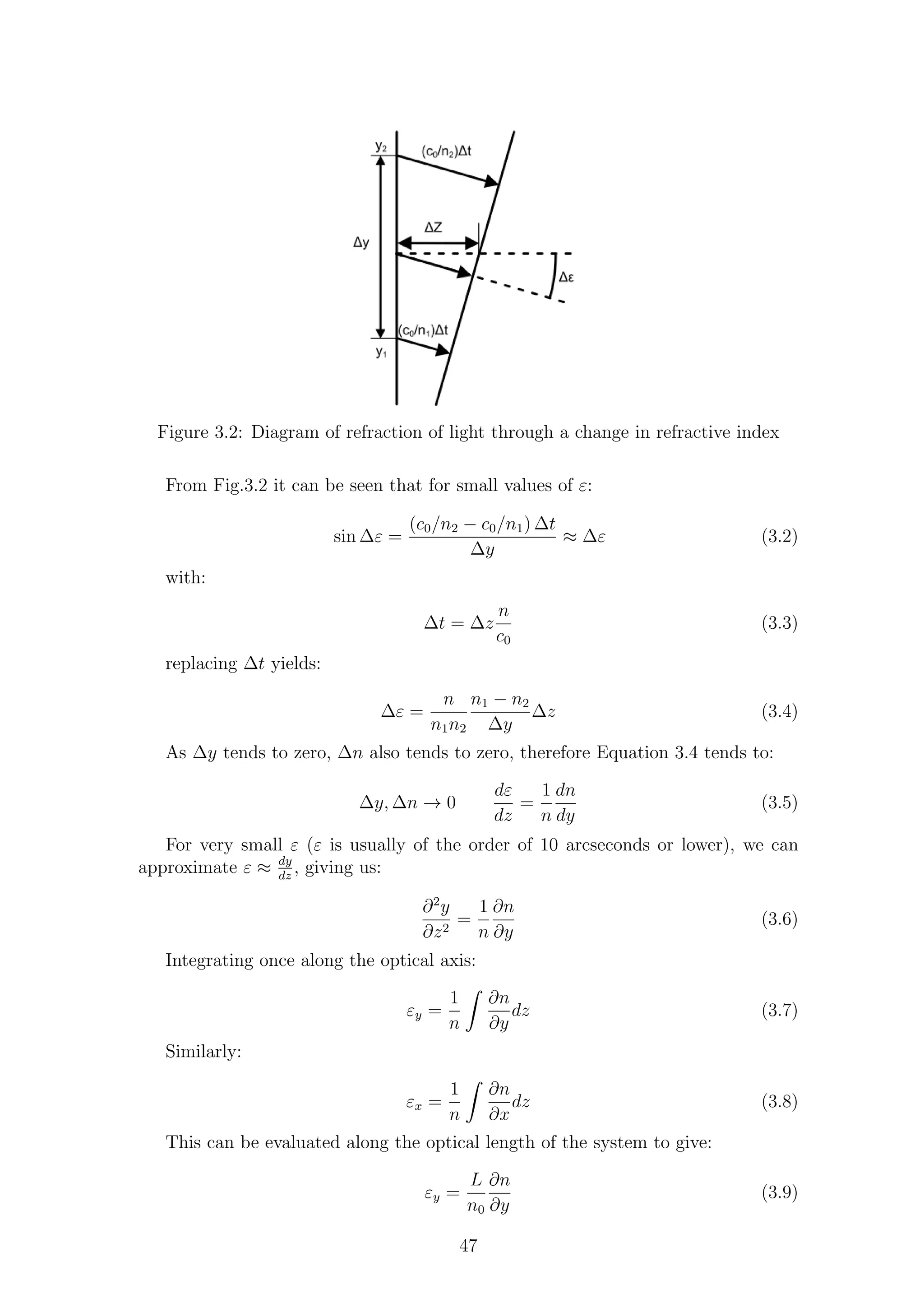
![εx =
L
n0
∂n
∂x
(3.10)
These equations are the basis for schlieren and shadowgraph systems as they
show the refraction of light with respect to change in refractive index normal to the
optical axis.
3.1.2.1 Shadowgraph Specifics
Shadowgraph imaging, as the name suggests, is based on the imaging of shadows.
The shadows are caused by the method shown in Fig.3.3. It shows that some light
has been refracted by a disturbance. Light slows in regions of higher refractive
index and speeds up in regions of lower refractive index. According to the induced
curvature of the wavefront seen in Fig.3.2, this means that light bends towards
regions of higher refractive index.
This explains the light pattern found in the shadowgraph of a flame seen by
Hooke [88], reproduced by the author on a wall illuminated by light reflected from
a nearby office block (Fig.3.4). The light is bent away from the flame as it has a
lower refractive index than the air around it, causing the inside of the plume to be
darker and the outside to be lighter.
Figure 3.3: Principle of shadowgraphy
As can be seen in Fig.3.3, the variation of ε with x or y is what is measured on
the screen. Differentiating Equations 3.9 and 3.10 gives:
dε
dy
=
L
n0
∂2
n
∂y2
(3.11)
dε
dx
=
L
n0
∂2
n
∂x2
(3.12)
This therefore shows that the shadowgraph technique is sensitive to the second
spatial derivative of refractive index, i.e. ray displacement. The only way to increase
the sensitivity of a shadowgraph system is to increase the distance between the
disturbance and the imaging plane; therefore, increasing ∆a. If this distance is too
large, flow features can become obscured, as large changes in density, such as shocks
or strong vortices, will appear as thick black shadows or become too blurred to give
the required information. This can be overcome by using the focused shadowgraph
technique, which is essentially the schlieren technique without a knife-edge.
48](https://image.slidesharecdn.com/4a6f74b5-6bbb-4ffd-b3f5-7486cdb057cd-150303082443-conversion-gate01/75/Mark-Quinn-Thesis-79-2048.jpg)
![Figure 3.4: Homemade shadowgraph of a lighter flame
Figure 3.5: Principle of focused shadowgraphy
If a point light source is used and the shadowgraph image is focused onto an
imaging plane (imagine Fig.3.6 without a knife-edge), then there will be no distur-
bances to image. Therefore, removing the knife-edge completely will produce what
is known as a focused shadowgraph. This is depicted in Fig.3.5. However, as ex-
tended light sources are finite in size, they have an associated depth-of-field. This
means that not all the field can be in focus at once. Biss et al. [109] showed that
if the camera focal plane and the test plane are coincident, almost no phenomena
are visible. However, as the distance between the focal plane and the test plane
is increased, the sensitivity of the focused shadowgraph is increased, albeit at the
cost of blurring the test plane. This increase in sensitivity can be introduced either
by deliberately defocussing the test plane or having an optical system with a short
depth-of-field. The trade-off between geometric blur and sensitivity yields the limit
of what can be measured using the focused shadowgraph technique. Section 3.1.5
will cover this in more detail.
49](https://image.slidesharecdn.com/4a6f74b5-6bbb-4ffd-b3f5-7486cdb057cd-150303082443-conversion-gate01/75/Mark-Quinn-Thesis-80-2048.jpg)
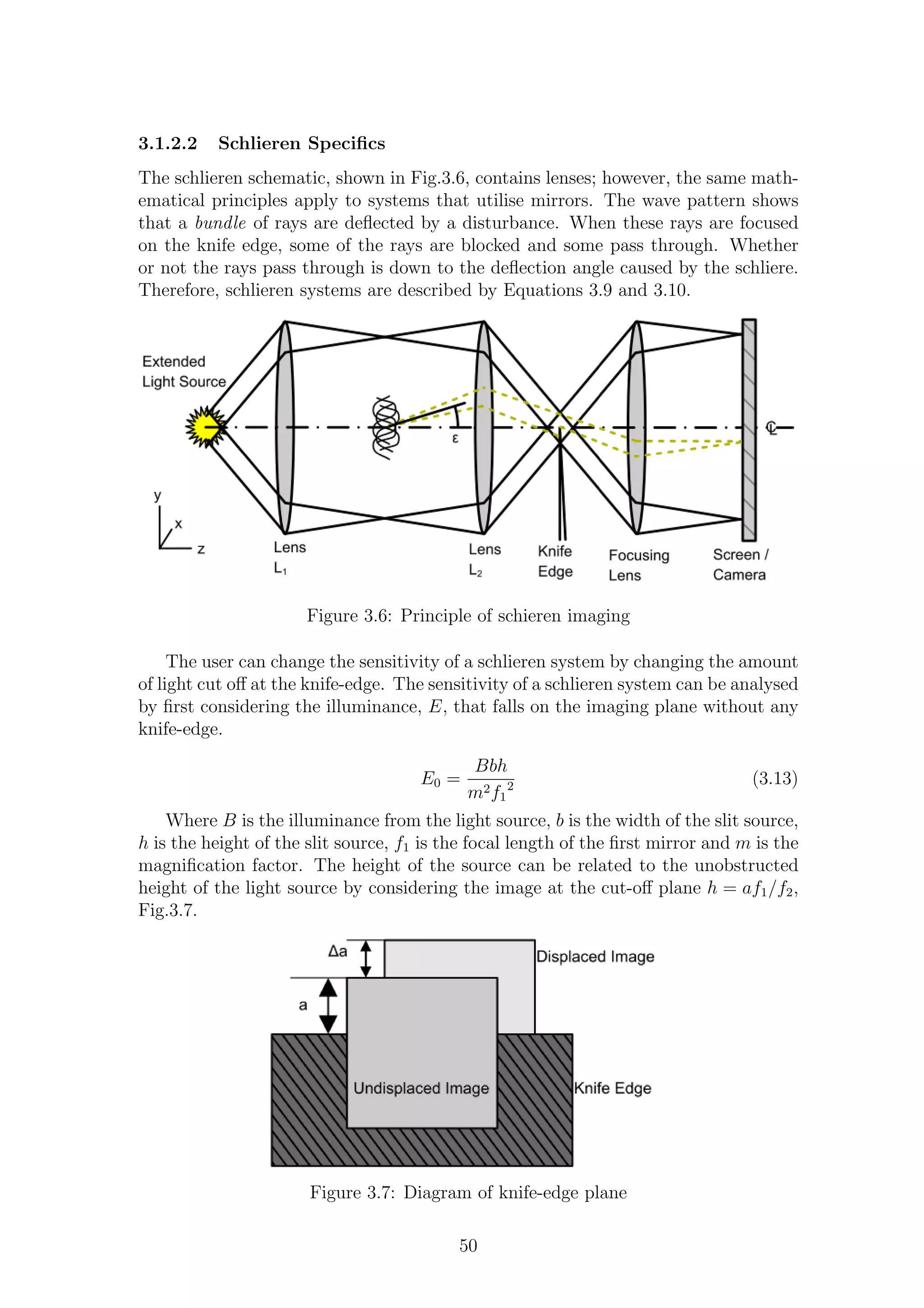
![E0 =
Bba
m2f1f2
(3.14)
Assuming a disturbance causes a refraction angle, εy, the image at the cut-off
plane will be displaced by ∆a = εyf2. Substituting ∆a for a in Equation 3.14 gives
the incremental change in illuminance on the imaging plane, ∆E.
∆E =
Bbεy
m2f1
(3.15)
Contrast is defined as the ratio of luminance difference to average luminance:
C ≡
∆E
E
=
f2εy
a
(3.16)
The sensitivity, S, of any system can be defined as the rate of change of output
with respect to input [107]. In terms of schlieren imaging, this can be defined as the
rate of change of contrast with respect to refraction angle:
S =
dC
dε
=
f2
a
(3.17)
From Equation 3.17, we can see that the sensitivity of a schlieren system can be
augmented either by reducing the unobscured image height (increasing the knife-
edge cut-off) or by increasing the focal length of the second lens or mirror. How-
ever, as the knife-edge cut-off is increased (a → 0) the overall measurement range
decreases [110]. The more the knife-edge is moved away from the 50% cut-off point
(i.e. a = h/2) the more nonuniform the measurement range becomes. As more light
is cut out, the darkening measurement range narrows and the lightening measure-
ment range widens. The system can then be described as over-ranged.
The ultimate limit on schlieren sensitivity is due to diffraction effects at the
knife-edge [111]. As a → 0, the knife-edge begins to act like a narrow slit and the
well-known diffraction effect begins to smear the image. Although the sensitivity
of the system is at its maximum, the resolving power is at its lowest. Therefore, a
compromise between these conflicting requirements is needed.
3.1.3 Limitations
Despite the capabilities of the schlieren and shadowgraph techniques, they are far
from the perfect diagnostic tool. The integration required to give Equations 3.9 &
3.10 assumes that changes along the optical axis are negligible. In three-dimensional
phenomena, this is not the case. Therefore, the integrative nature of both schlieren
and shadowgraph techniques mean that they are more applicable to two-dimensional
rather than three-dimensional phenomena. This can also give erroneous results if
there are any disturbances along the optical path apart from the test section. This
can be especially apparent when using a high-intensity arc lamp, as the convection
currents caused by the high temperatures involved can appear in the final schlieren
image.
Schlieren and shadowgraph techniques are regarded as qualitative techniques
rather than quantitative. It is true that it is extremely difficult to extract quan-
titative measurements of density from these techniques (interferometry is usually
51](https://image.slidesharecdn.com/4a6f74b5-6bbb-4ffd-b3f5-7486cdb057cd-150303082443-conversion-gate01/75/Mark-Quinn-Thesis-82-2048.jpg)
![required for that [112] [113]). However, other information can be gained, such as
shear layer spreading, wave propagation speeds and shock wave angles.
3.1.4 Applications
Schlieren systems are applicable to almost any type of flow, provided optical access is
available. This ranges from investigating shock waves, shear layers and turbulence
to seeing sound, as they can often be sensitive enough to pick up acoustic waves
[94] or even weaker phenomena [114]. They can also be used to see heat transfer
patterns, combustion and even microscopy.
Colour filters can be used as source masks as a replacement for a knife-edge
in a schlieren setup to produce colour images. Colour schlieren has the advantage
that it can not only show variations in refractive index very clearly, but if a two-
dimensional source mask is used, it can also give information about the direction
of the gradient [115]. Howes describes this as `‘the principle benefit of color is in
labeling the refraction with respect to direction and magnitude” [116].
If a fluid of different density can be introduced into the flow, it will be very
visible using schlieren and shadowgraph. Several researchers have made great use of
this fact (Pierce [117] and Roshko [57] are two excellent examples of this method).
Schlieren and shadowgraph systems can be used to create x-t diagrams (see
Section 2.2.1) by extracting a line of pixels from a stack of schlieren images and
superimposing them above each other. This can be completed quickly and easily
and is known as image re-slicing. From x-t diagrams, shock propagation speeds can
be calculated by measuring the gradient of the line present.
Figure 3.8: x-t diagram for a Mi = 1.46 shock
3.1.5 Setup
The schlieren and shadowgraph system used in this project is the ubiquitous Z-style
system. Illumination comes from an in-house-built 300W Xenon arc lamp. The
beam expands towards a hemispherical lens which condenses the beam to a slit
placed at the focal distance from the first mirror. The two mirrors are 8 inches in
diameter at f# = 4.5, giving a focal length of 3 feet. The imaging device is the
Shimadzu HPV-1, capturing at 250 kfps with an exposure time of 2µs. The HPV-1
is a fast frame CCD camera with an 8-bit dynamic range. Despite the powerful light
source, the full dynamic range of the HPV-1 could not be utilised with a 2µs exposure
time. However, a longer exposure time would have blurred the moving shock waves,
and so 2µs was found to be the best compromise between these requirements.
In order to eliminate the effect of coma and minimise astigmatism, the angles
shown in Fig.3.9 are: δ1 = δ2 = 3◦
. Astigmatism is a smearing effect caused by
having different optical lengths along the optical axis and the edge. This arises due
to the tilting of the mirrors seen in Fig.3.9. It is not possible to eliminate the problem
52](https://image.slidesharecdn.com/4a6f74b5-6bbb-4ffd-b3f5-7486cdb057cd-150303082443-conversion-gate01/75/Mark-Quinn-Thesis-83-2048.jpg)
![of astigmatism in Z-style schlieren setups; however, it is possible to minimise them
by having the smallest angle, δ, possible. The difference in optical path length is
given by Equation 3.18.
∆f = f
sin2
δ
cos δ
= 2.77mm (3.18)
This indicates that, for this system, astigmatism is not a significant problem
[107].
Figure 3.9: Schlieren setup
The beam is the passed through then test section to the second mirror and on
to the knife-edge. Two optical zooms will be employed in this project, with careful
attention paid to the depth-of-field in each case. The focusing lens for the full-field
images is a combination of 55mm +1 and +2 diopter macro lenses. These lenses
have an optical power of 3, giving them a focal length of 0.33m. For the close-up
images, the beam was allowed to expand further from the knife-edge before passing
through a +1 diopter lens to produce a sharp image. These lens combinations
were deliberately chosen to have a shallow depth-of-field. The imaging device is
the Shimadzu HPV-1. The sensor of this camera is 20.7 x 17.2 mm in size (pixel
size 66.7µm). The circle of confusion of the optical system is set to be the pixel
size of the HPV-1. This allows us to estimate the depth-of-field of the system once
we calculate the hyperfocal distance, H (Eq.3.19) and eventually the depth-of-field
[118].
H =
f2
f#c
+ f (3.19)
Where f is the lens focal length, f# is the f-number and c is the circle of
confusion. Now we can calculate the near (Dn) and far (Df ) distances of acceptable
sharpness
Dn =
s(H − f)
H + s − 2f
(3.20)
53](https://image.slidesharecdn.com/4a6f74b5-6bbb-4ffd-b3f5-7486cdb057cd-150303082443-conversion-gate01/75/Mark-Quinn-Thesis-84-2048.jpg)
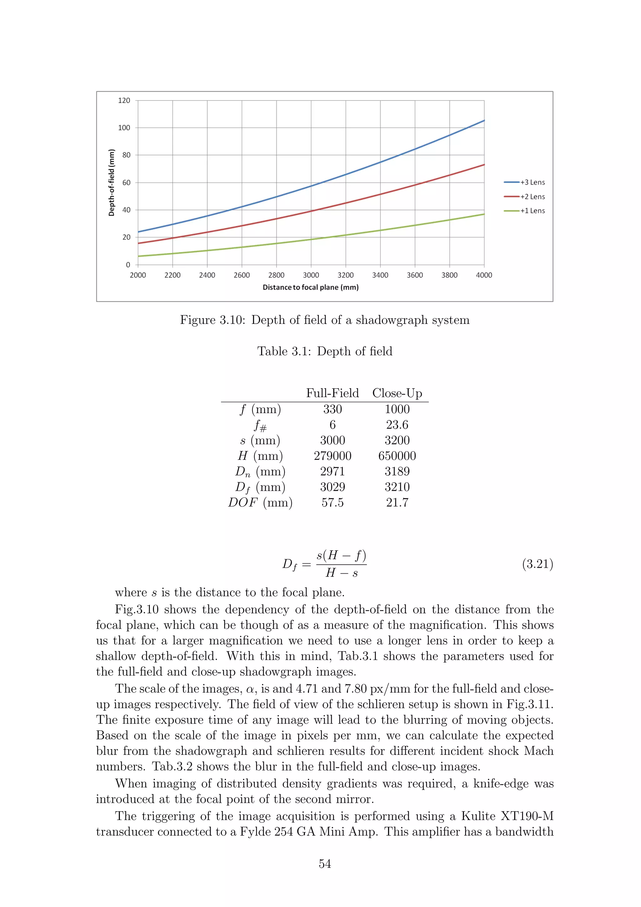
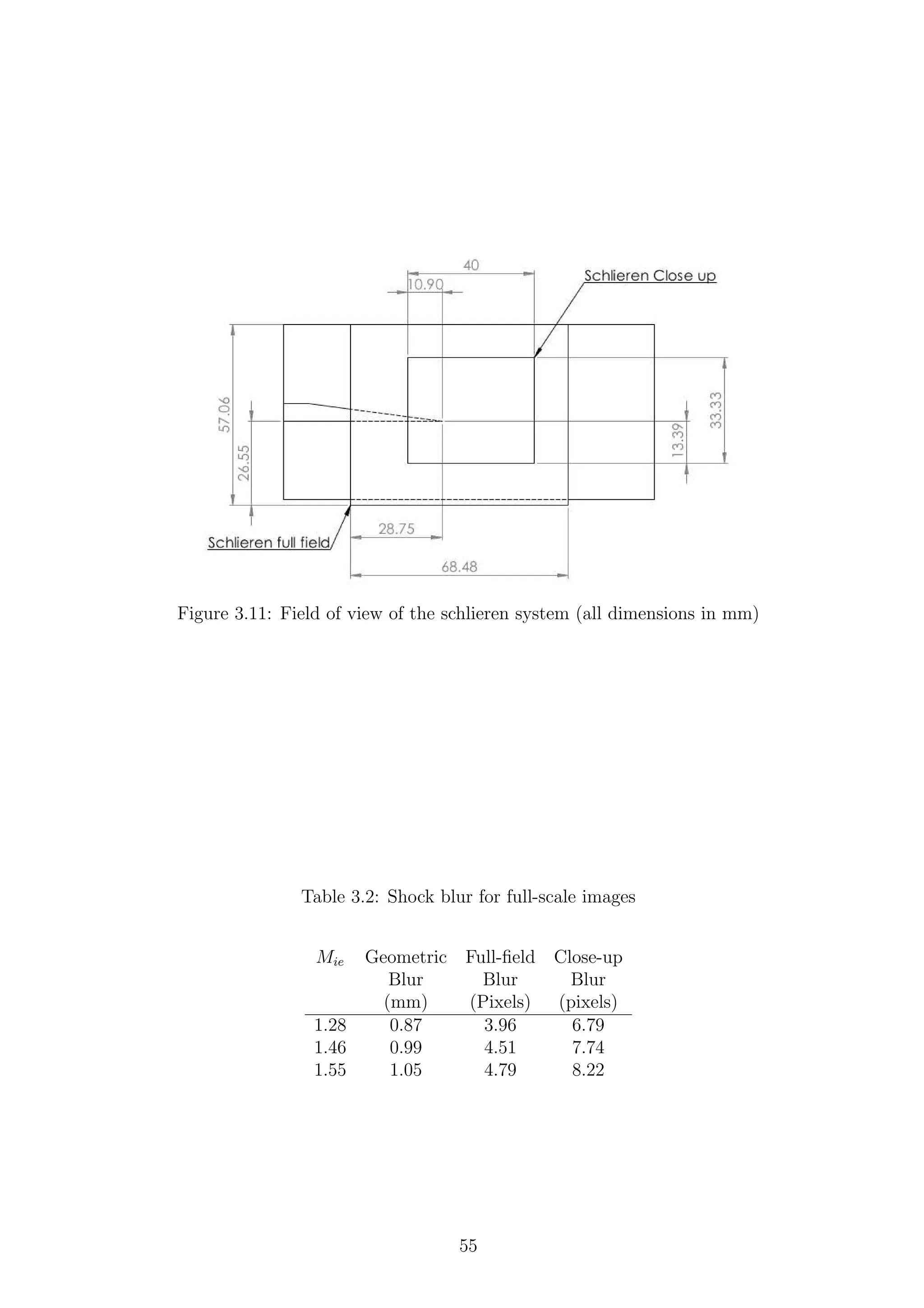
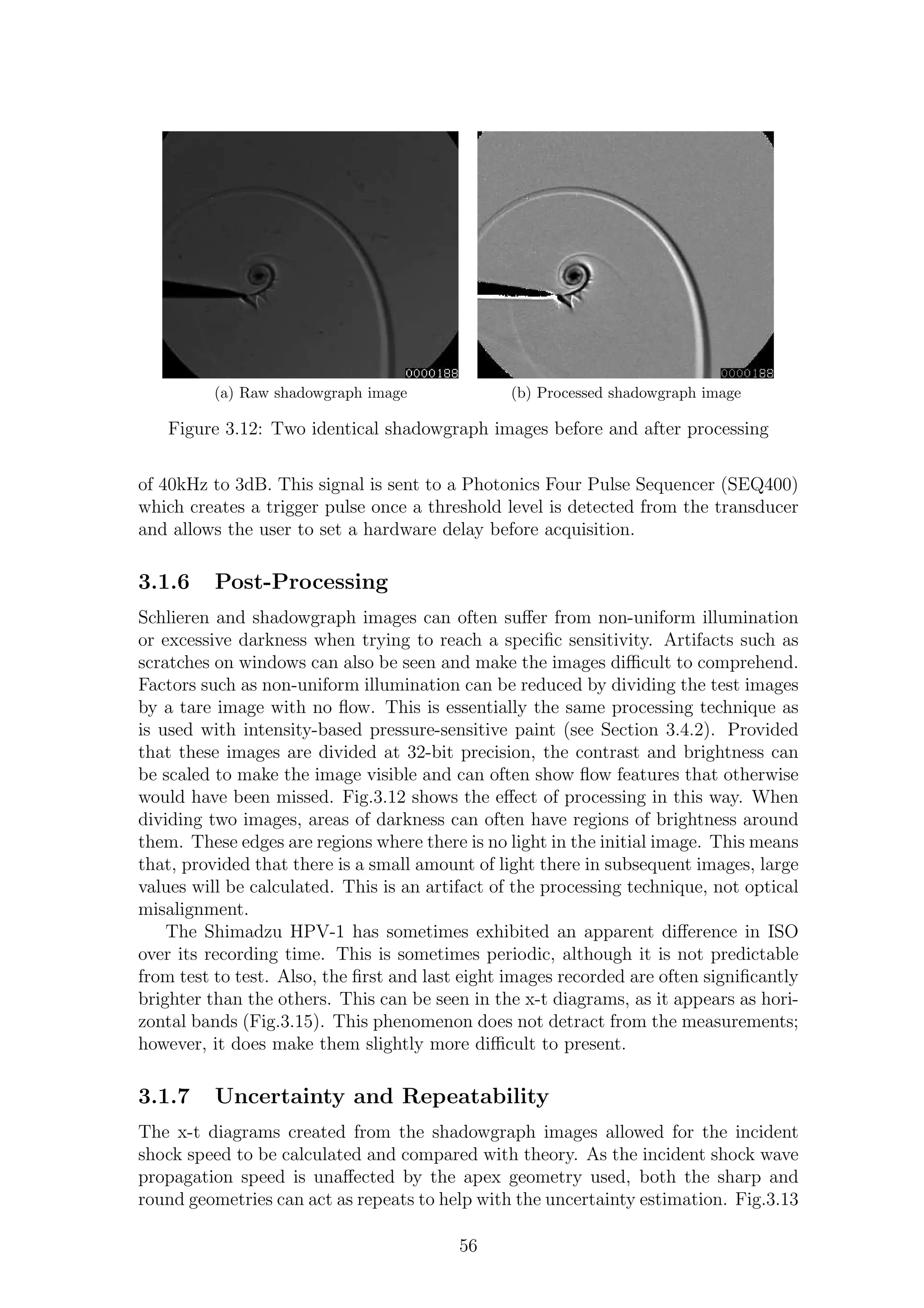
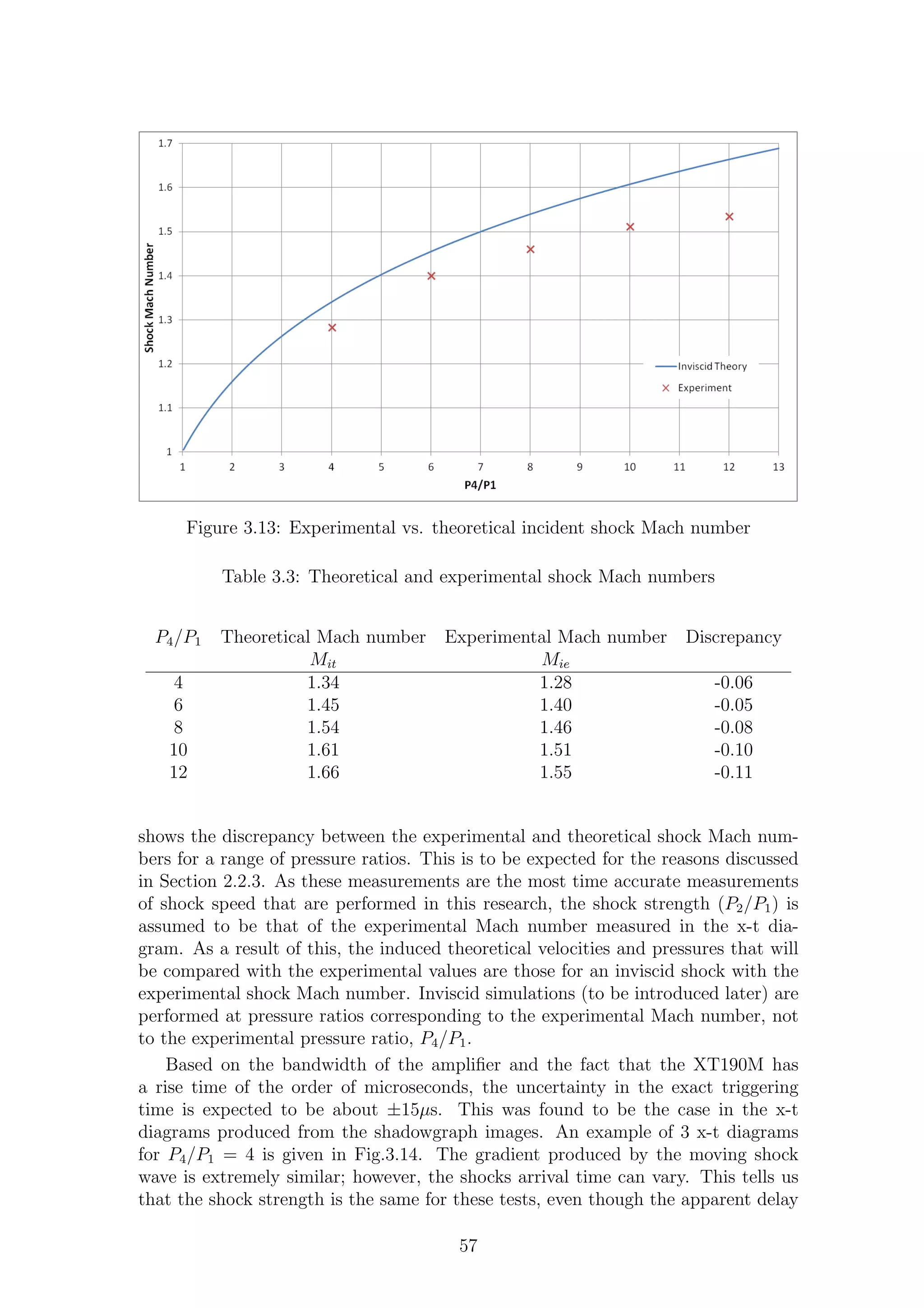
![(a) Run 1 (Shadowgraph)
(b) Run 2 (Shadowgraph)
(c) Run 3 (Schlieren)
Figure 3.14: Experimental x-t diagrams resliced from 101 frames
is different. The curved waves appearing at the top of the x-t diagrams are reflected
diffracted waves returning from the upper surface of the test section. The shock
position is only measured until the reflected expansion wave has reached the reslice
line (which is as low as it can be in the image). Abate & Shyy refer to this as when
the shock becomes critical [79]. It physically means that the shock wave is no longer
planar and will therefore have a different propagation velocity.
Fig.3.15 shows the shock position as a function of time for both full-field and
close-up tests for all three pressure ratios tested. The gradients of these lines rep-
resent the propagation speed of the shock wave. For each pressure ratio, five shock
speeds were analysed and the statistical uncertainty is presented in Tab.3.4. The
bias error is a combination of incorrectly estimating the scale of the images by .5
mm and incorrectly estimating the shock wave position by 2 pixels. The random
errors are calculated to 95% confidence (1.96σ).
Estimating the uncertainty in velocity estimations from schlieren measurements
is relatively simple. The images are scaled so that
ximage
α
= xreal, where α is the
scale of the images in pixels per mm. Substituting this into the simple equation
58](https://image.slidesharecdn.com/4a6f74b5-6bbb-4ffd-b3f5-7486cdb057cd-150303082443-conversion-gate01/75/Mark-Quinn-Thesis-89-2048.jpg)
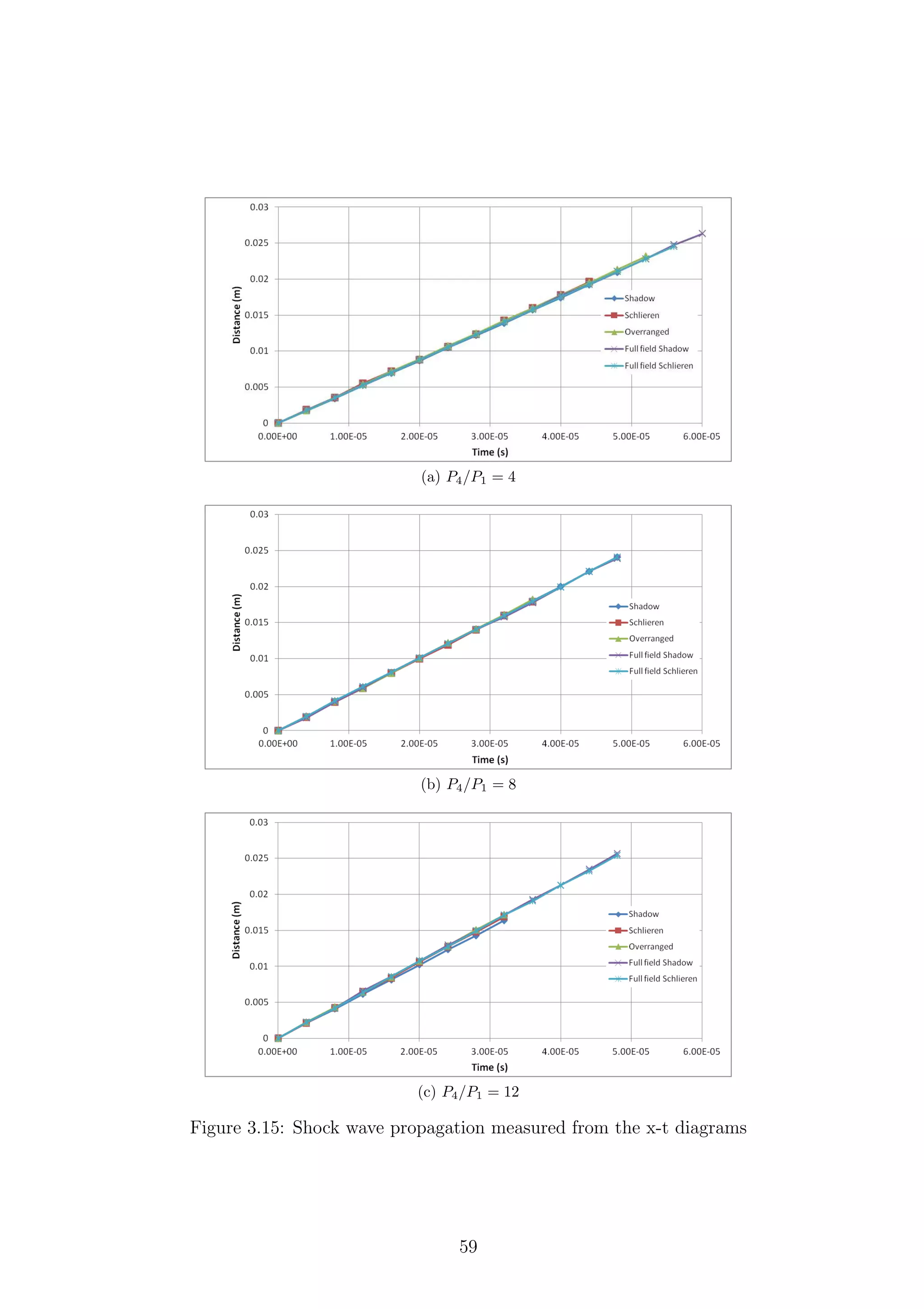
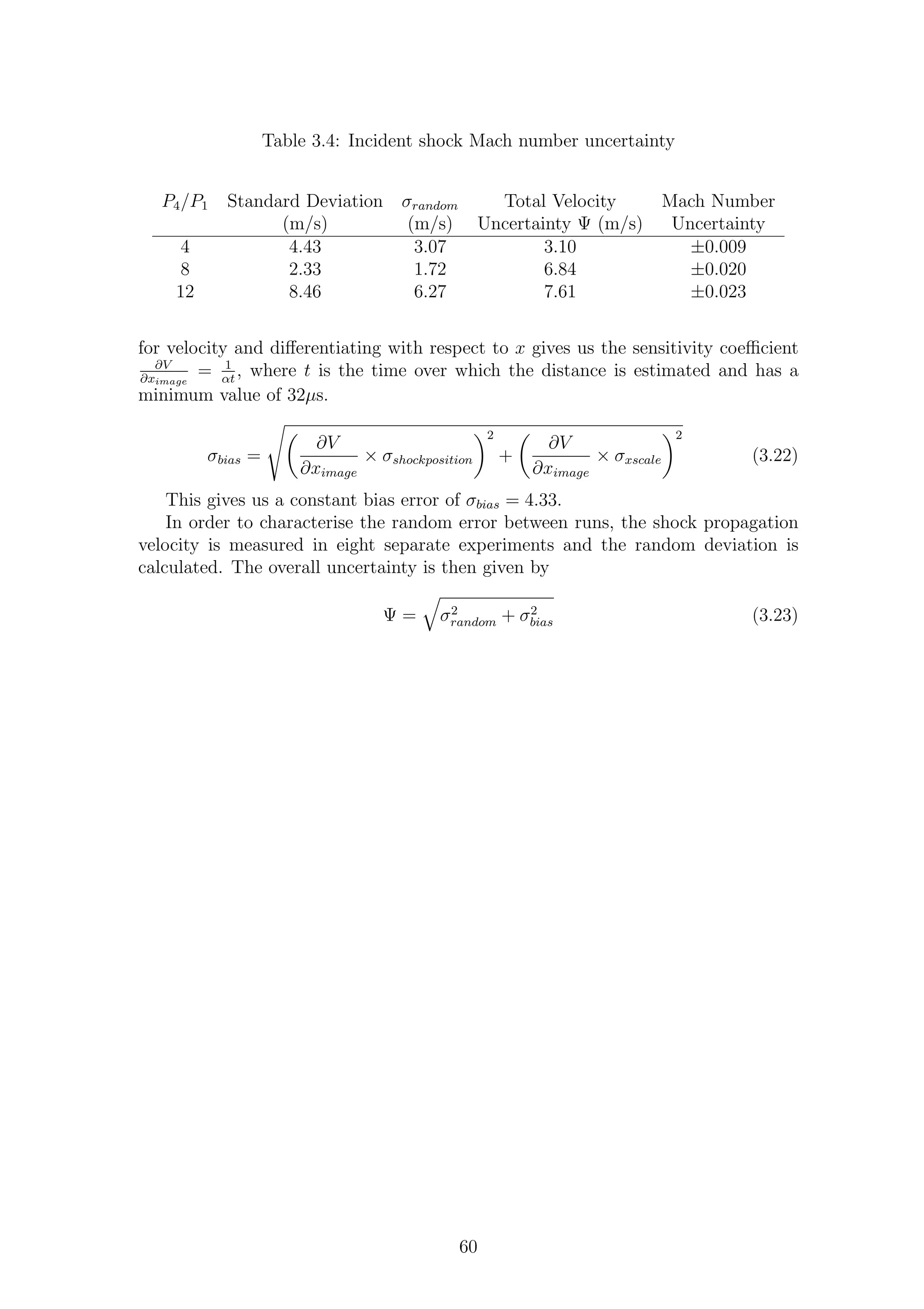
![3.2 Particle Image Velocimetry (PIV)
Particle Image Velocimetry (PIV) is an essentially non-intrusive method3
of mea-
suring the velocity components of a whole flow field in one test. This gives it
a distinct advantage over more traditional methods of measuring point velocities,
such as hot-wire anemometry (HWA), laser Doppler anemometry (LDA) and pitot
measurements. PIV is capable of capturing phenomena which are almost impossible
to capture with traditional point methods, such as the complex structures of shed
vortices. This increase in spatial resolution compared to traditional techniques is a
similar leap forward to the increased resolution of PSP over pressure tappings.
3.2.1 History and Development
The earliest recording of particle-based flow diagnostics can be traced back to the
work of Ludwig Prandtl in 1904 [119]. In this early work, a suspension of mica
particles in water was used to visualise the starting flow behind an airfoil. This led
him to develop theories about the starting vortices and also to show the effects of
flow separation and vortex streets.
Over the past 20 years PIV has become a powerful tool of scientists exploring fluid
flows. Initial attempts to quantitatively measure the velocity of a fluid using seeder
particles were performed using what is now known as laser speckle velocimetry. This
technique involved measuring the interference fringes created by pairs of displaced
speckles [120]. Laser speckle velocimetry requires the density of particles in the fluid
to be extremely high. This can lead to two-phase flow effects, which is not usually
the intention.
Modern PIV systems, previously called high-density PIV, have evolved from low-
density PIV, also known as particle-tracking velocimetry (PTV). The distinction is
based upon the concentration of seeding particles in the flow. PTV uses simpler
image processing algorithms than PIV, as there are much fewer particles in the flow.
The nature of PIV means that high-speed applications are more challenging than
low-speed applications, due to the more complicated imaging systems involved and
expensive, high-energy, double-pulsed lasers.
When compared with integrative diagnostic techniques such as schlieren imaging,
PIV has the advantage that the flow can be imaged in a 2D plane, showing structures
that could otherwise be missed. PIV is not only capable of measuring two velocity
components, but it is also capable of capturing all three velocity components in a
given plane by use of stereoscopic imaging. Recent advances in PIV technology have
shown the development of tomographic PIV, which involves using four cameras to
measure all three components of velocity in a given laser volume rather than a laser
plane [121]. Tomographic measurements require an enormous amount of processing
power and data storage and currently have not been applied to high-speed flow such
as the ones investigated in this project. Despite tomographic PIV appearing to be
the future of particle-based flow diagnostics, regular two-dimensional PIV will be
used in this project due to its robustness and lower processing time.
3
The use of large seeder particles can be intrusive, altering the flow; however, this can be avoided
by a proper choice of seeding material.
61](https://image.slidesharecdn.com/4a6f74b5-6bbb-4ffd-b3f5-7486cdb057cd-150303082443-conversion-gate01/75/Mark-Quinn-Thesis-92-2048.jpg)
![3.2.2 Theory
PIV is based on the displacement of particles suspended in the flow between two
images. Given a known delay between consecutive images and assuming that indi-
vidual particles can be identified in both images, the velocity of each particle can
be calculated. Assuming that the particles are small enough not to affect the flow,
but to accurately follow it, the velocity of the flow can be calulated. The simplicity
of the basic explanation above understates the complexity of the systems and math-
ematics involved in PIV experiments. A full derivation of the mathematics of PIV
and the image processing involved is beyond the scope of this project; however, an
error analysis and detailed discussion of seeder particle characteristics will follow.
The flow is illuminated by a high-power, double-pulse, typically ND:YAG laser
with a pulse energy of approximately 400mJ. This laser is passed through a series
of lenses to create a laser sheet. The flow is seeded with light-scattering particles.
These particles scatter light towards the imaging device, usually a high-speed cam-
era with a filter to cut out background noise. The imaging device records two images
separated by a short time (∆t). These images are then broken down into smaller
sections, called interrogation regions, to be analysed by the data acquisition system.
The smaller the size of the interrogation region, the smaller the flow features that
can be captured. However, if the interrogation region is too small then there is
the possibility of the particle moving from one window to another, causing large
errors. Some researchers [122] [123] have applied an iterative grid refinement tech-
nique based on the multi-grid method. This adaptive grid is crucial in high-speed
applications of PIV, as the presence of sharp gradients (i.e. shock waves) tends to
be smoothed out if large interrogation regions are used [124].
In order to ascertain the velocities of the particles in the flow, the two images
must be compared. The process of determining which particle has travelled to where
inside the interrogation region is called cross-correlation. This is a statistical analysis
that shows the probability that the particles in each image have been correctly
identified.
3.2.3 Seeder Particles
Seeder particles have two functions in PIV experiments:
• To follow the path of the flow as closely as possible
• To scatter light to the PIV imaging device
These two requirements are conflicting in that smaller particles follow the flow more
closely but larger particles scatter more light. Some seeder particles such as TiO2
perform both of these functions very well; however, they are difficult to seed into the
flow reliably. Therefore, the selection of seeder particles is a compromise between
these requirements and ease of use. Low-density particles are the best option for
vortical flows, as centrifugal forces tend to eject heavy particles [125].
The analysis of the seed particles’ performance as flow tracers is based upon
Stokes’ drag law and is shown by Raffel et al. [126]. Equation 3.24 shows the slip
velocity, Us, which is the difference between the seed particle velocity (Up) and the
flow velocity (U). The particle diameter is dp and the particle density is ρp.
62](https://image.slidesharecdn.com/4a6f74b5-6bbb-4ffd-b3f5-7486cdb057cd-150303082443-conversion-gate01/75/Mark-Quinn-Thesis-93-2048.jpg)
![This equation is valid for particles bigger than 1 micron in diameter; however,
below this size, the Knudsen number (based on the particle diameter Kn = λ/dp)
becomes sufficiently large that the assumption of continuum dynamics is no longer
valid [127]. In this case, Stokes’ drag law can be corrected using Cunninghams’
slip correction factor, Cu, which is an empirical relationship (Equation 3.25) based
on Knudsen number. If the seed particles are even smaller, i.e. smaller than the
mean free path length, then Brownian motion should be taken into consideration
[127]. The response of the seed particle to a step change in velocity, such as a shock
wave, can be modelled by a single exponential, as in Equation 3.26, where τs is the
relaxation time given by Equation 3.27.
Us = Up − U = dp
2 (ρp − ρ)
18µ
Cu (3.24)
where,
Cu = 1 + Kn A + Be− C
Kn (3.25)
where A, B and C are empirically derived constants. Jennings [128] showed values
of these constants estimated by previous researchers and showed their effect on Cu.
The values estimated by Jennings will be used in these calculations: A = 1.252,
B = 0.399, C = 1.10.
Up (t) = U 1 − e− t
τs (3.26)
τs = dp
2 ρp
18µ
Cu (3.27)
Melling [129] shows similar results to those in Table 3.5, stating that for super-
sonic flows the particle diameter should be sub-micron, otherwise the velocity lag
becomes prohibitively large. It was shown computationally by Samimy & Lele [130]
that the size of the particles shown in Table 3.5 should faithfully follow the flow for
the velocities of interest in compressible shear layer experiments. However, more
recent studies by Ragni et al. [131] and Ghaemi et al. [132] have shown that, even
when using nanoparticles, the relaxation time can still only be as low as ≈ 0.3µs.
Clearly, it is advantageous to have a relaxation time which is as short as possible.
However, smaller particles scatter less light, making it much harder to image them.
This is the reason that applications of PIV in gas flows require more powerful and
therefore more expensive lasers than liquid flows.
The values in Tab.3.5 are based on a normal shock in an isentropically expanded
Mach 1.5 flow with an initial temperature of 300K. This gives a shock strength of
2.46, giving a velocity drop of 200 m/s. The relaxation distances shown in Tab.3.5
are for steady flow. Fig 3.16 shows the dependency of the response characteristics
on particle diameter for various materials. If the flow is psuedo-steady, in that it is
oscillatory but can be time-averaged, the response times above still apply. However,
if the flow is transient, as in the case of shock wave diffraction, a slightly more
involved approach must be used.
During the characteristic rise time shown above, the particle is accelerating to-
wards the flow velocity. However, if the flow is induced by a moving shock wave, a
63](https://image.slidesharecdn.com/4a6f74b5-6bbb-4ffd-b3f5-7486cdb057cd-150303082443-conversion-gate01/75/Mark-Quinn-Thesis-94-2048.jpg)
![Table 3.5: Relaxation Characteristics of Seeder Particles
Particle ρp dp τs
[Kgm−3
] [µm] [µs]
Al2O3 3970 2 51.6
1 13.4
0.5 3.55
0.1 0.23
TiO2 3500 2 45.5
1 11.8
0.5 3.19
0.1 0.21
CaCO3 2830 2 36.8
1 9.57
0.5 2.58
Glass Balls 2600 2 3.38
1 8.79
0.5 2.37
Olive Oil 970 2 12.6
1 3.28
DEHS 912 2 11.9
1 3.08
theoretically instantaneous velocity change, the shock wave has propagated further
downstream during the rise time. In order to calculate the shock spreading distance
(i.e. the distance over which an instantaneous velocity change is spread), first we
must integrate Equation 3.26 with respect to time to attain the distance travelled
in the relaxation time, xr.
xr = U t + τs 1 − e− t
τs (3.28)
This distance should then be subtracted from the distance the shock has travelled
in this time. Fig.3.16b shows the spreading of a shock wave by particles commonly
used in PIV. The shock Mach number of this analysis is 1.34, giving an induced
velocity of ≈ 170 m/s. It should be noted that some of the particles cannot be
reliably generated at sizes smaller than those shown in Fig.3.16.
As shown in Table 3.5, olive oil is an excellent seeder material as it has very good
relaxation characteristics. Olive oil can be atomised by numerous methods; however,
a Laskin nozzle is the simplest and the most cost-effective. Olive oil is used as the
seeder material in the majority of experiments at the University of Manchester, as
it is reliable and simple to use. However, the relatively large particle size limits the
application of liquid seeder materials in extremely high-speed or transient flows; as
a result, solid particles are often used.
Generation of uniform seeder particles is often difficult to achieve when seeding
with solid particles such as Al2O3. Although solid seeder material is generally bought
in bulk from a supplier to sizes as small as 15nm, when they are seeded into the
64](https://image.slidesharecdn.com/4a6f74b5-6bbb-4ffd-b3f5-7486cdb057cd-150303082443-conversion-gate01/75/Mark-Quinn-Thesis-95-2048.jpg)
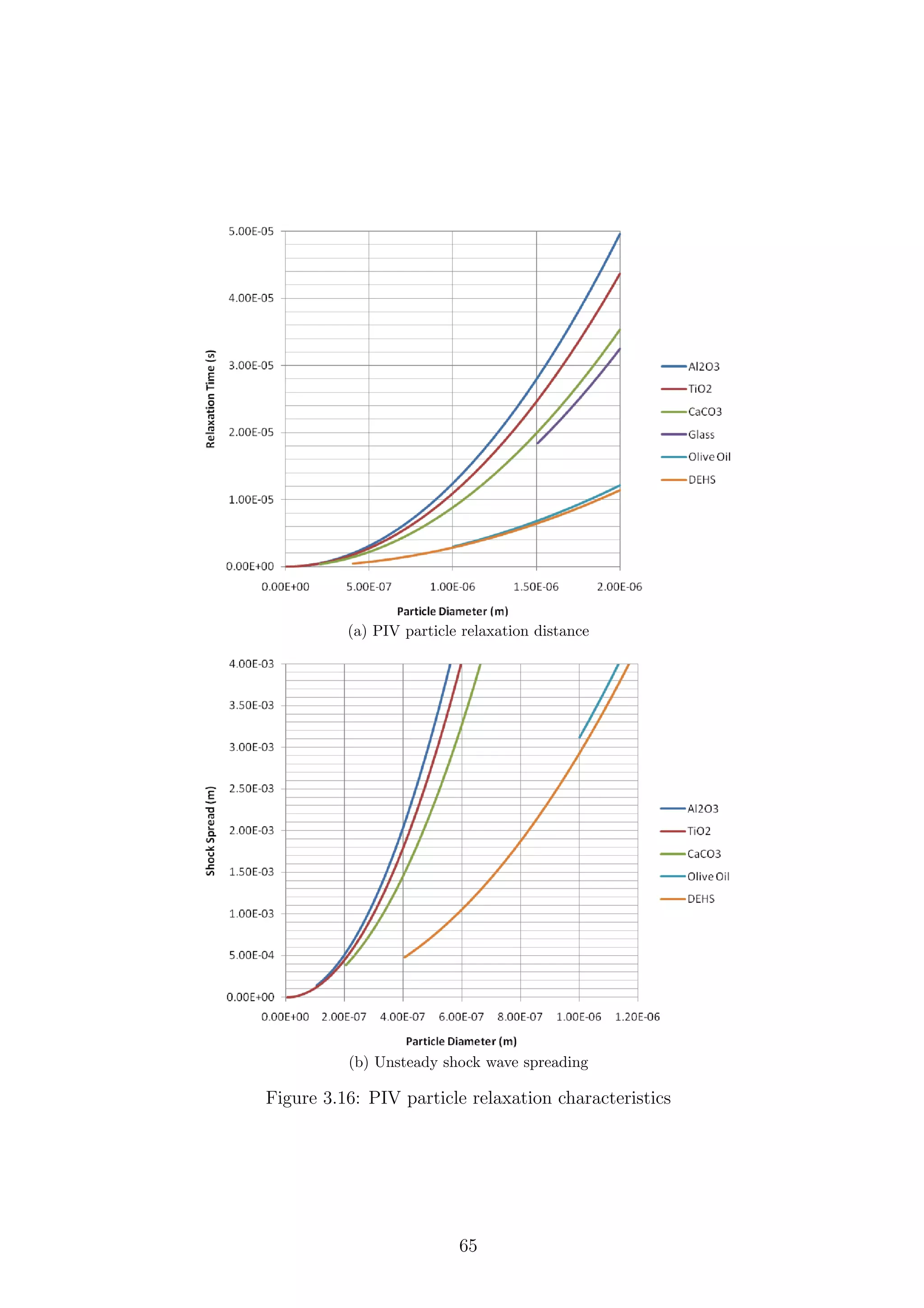
![flow they can agglomerate due to their hydrophilic nature to form larger, irregular
particles (see Fig.3.17). Ragni et al. [131] attempted to overcome this problem by
baking the seeding material in an oven before testing, hoping to dry the material
further. This proved successful in reducing the relaxation time of particles, with the
curious exception of the smallest TiO2 particles. Solid seeder material used in this
study will be baked overnight at 350K before testing. Both Fig.3.17a and Fig.3.17b
have been passed through the seeder described in Section 3.2.6; however, the particle
drum had been baked for Fig.3.17b and was not for Fig.3.17a.
(a) Particles before baking (b) Particles after baking
Figure 3.17: Laser confocal microscope images of Al2O3 particles with and without
baking
According to Melling [129], the ideal concentration of seeder particles for high-
speed measurements should be ≈ 15 particles per interrogation volume. Seeding
open-ended, continuous high-speed wind tunnels with an adequate number of seeder
particles is extremely challenging due to the flow rates of the atomisers involved.
However, seeding shock tubes and variants thereof (Ludwieg tubes, shock tunnels
etc.) is simpler as, the test section can be seeded before the test run [133].
3.2.4 Limitations
Despite the excellent data that can be captured with PIV systems, they do have
some limitations. Laser repetition rate sets the ultimate capture limit for a sys-
tem. Modern double-pulse lasers are capable of 10 kHz. The ∆t between images
is ultimately set by the imaging device. This sets the maximum velocity that can
be measured in a given interrogation region. The resolution of the imaging system
limits the number of vectors that can be produced. In high-speed flow, this is rarely
a reachable limit as the limit is usually set by the density of seeder particles. Two-
dimensional PIV is highly susceptible to out-of-plane velocity components, which
often mean that the particles can pass out of the laser sheet between the frames.
66](https://image.slidesharecdn.com/4a6f74b5-6bbb-4ffd-b3f5-7486cdb057cd-150303082443-conversion-gate01/75/Mark-Quinn-Thesis-97-2048.jpg)
![3.2.5 Applications
Researchers have applied PIV across a wide range of speed regimes, from incom-
pressible to hypersonic. Hale et al. [134] [135] applied PIV to a induced jet from a
plasma actuator in quiescent air, capturing velocities ranging from 0 − 8m/s. Ragni
et al. [136] applied PIV to a transonic airfoil with localised supersonic regions. Using
the isentropic relations, Ragni et al. were able to estimate the surface pressure on
each side of the airfoil and as a result estimate the lift, drag and pitching moment.
Application of PIV to high-speed flow, more relevant to this project, has been
performed despite the technical challenges involved. Gongora-Orozco et al. [41]
successfully applied PIV to shock tube flows with and without co-flow jets, albeit
using olive oil as the seeder material.
High-velocity shock tunnel flows have been investigated by Haertig et al. [137].
By their nature of compression by two normal shocks, shock tunnels have extremely
high enthalpy flow conditions that resemble actual hypersonic flight conditions. The
velocity of the flow after a convergent-divergent nozzle was ≈ 1500 m/s. The level
of accuracy of the PIV measurements was extremely good (more than 99% accu-
rate); however, the spatial resolution was limited. The improvement in laser and
CCD technology since this research has led to research of similar velocities with
significantly higher spatial resolution [124].
Schrijer et al. [122] applied PIV to hypersonic flow (Mach 7) over a double-
ramp generated by a Ludwieg tube. This research used the adaptive grid method
of interrogation (as mentioned in Section 3.2.2) and showed a freestream velocity
discrepancy of 10% with isentropic theory. This is unsurprising given the high Mach
number of the flow; however, the flow structures which were visible correlated well
with schlieren images. Later research by Schrijer et al. [138] applied stereoscopic PIV
to the same experimental rig and compared the results with CFD. Boundary/shock
layer measurements of the flow showed highly complex structures such as G¨ortler
type vortices and a large separation bubble.
Not only have freestream flow fields been investigated using PIV, but shock
wave turbulent boundary layer interactions have also been investigated by Humble
et al. [139] in a Mach 2.1 flow. The region of investigation in this research was
16mm high and 5mm wide. Despite this small area, the flow was well resolved
and highlighted instantaneous regions of reversed flow and unsteady shock wave
movement. Later work using a high-speed tomographic PIV system by Humble et
al. [140] detailed highly complex three-dimensional vortical structures. The results
were very promising; however, the author did highlight the technical difficulties
associated with this technique, such as the prohibitively large data storage required.
In addition to yielding quantitative velocity data, PIV can also give excellent
flow visualisation that is not readily available from other techniques. The particles
seeded into the flow will tend to be ejected from vortex cores, no matter how low
their inertia is. This means that we should expect the raw PIV images to highlight
the edges of any vortices present in the flow (see Fig.3.22), although this means that
it will not be possible to obtain any quantitative data in this region.
67](https://image.slidesharecdn.com/4a6f74b5-6bbb-4ffd-b3f5-7486cdb057cd-150303082443-conversion-gate01/75/Mark-Quinn-Thesis-98-2048.jpg)
![3.2.6 Setup
Figure 3.18: Position of laser sheet in shock tube
A light sheet was shone down the centre-line of the shock tube, as shown in Fig.3.18.
This light sheet was created using two lenses, and a slit-like cut-off was used to
produce a more top hat-like profile. The position of the second lens controlled the
position of the waist of the sheet. The waist of the beam should not be within the
measurement area of the experiment, as it is this area of the beam that exhibits the
largest gradients in power [141]. In this setup, the waist of the beam was before the
test section.
Several measurements were taken at different spanwise locations to ensure the
two-dimensionality of the flow. The flow measurements were indistuingishable at all
of the spanwise locations. This concurs with the conclusion at the start of Section
5.1 that two-dimensional simulations are suitable for investigating this flow.
The system often used at The University of Manchester is the TSI high-speed,
high-resolution particle image velocimetry system. This system consists of the Pe-
gasus double pulse laser with the Photron APX-RS as the imaging device, which has
a resolution of 512 x 512 pixels. Initial tests were performed using this system with
olive oil as the seed and it was found that ∆tmin = 2.5µs. This minimum value was
imposed by the interframe time of APS-RX. It was found from these initial tests
that olive oil droplets do not respond quickly enough to accurately capture the flow,
and that the spatial and temporal resolution of the APX-RS is not sufficient to give
accurate enough results.
The only PIV system available with a small enough ∆t was the LaVision Flow-
Master with an Imager Pro X2M camera coupled with a Litron Nano-L-200-15 PIV
Nd:YAG laser. This system allows ∆tmin = 110 ns and has an image resolution of
1600 x 1200 pixels. The field of view of the PIV system is shown in Fig.3.19. Values
of ∆t were changed from 1µs for P4/P1 = 4 to 0.5µs for P4/P1 = 8 and 0.3µs for
P4/P1 = 12. This kept the effective CFL number down to manageable values. Solid
Al2O3 nanoparticles were passed through the SciTech Consultants PS-10 powder
68](https://image.slidesharecdn.com/4a6f74b5-6bbb-4ffd-b3f5-7486cdb057cd-150303082443-conversion-gate01/75/Mark-Quinn-Thesis-99-2048.jpg)
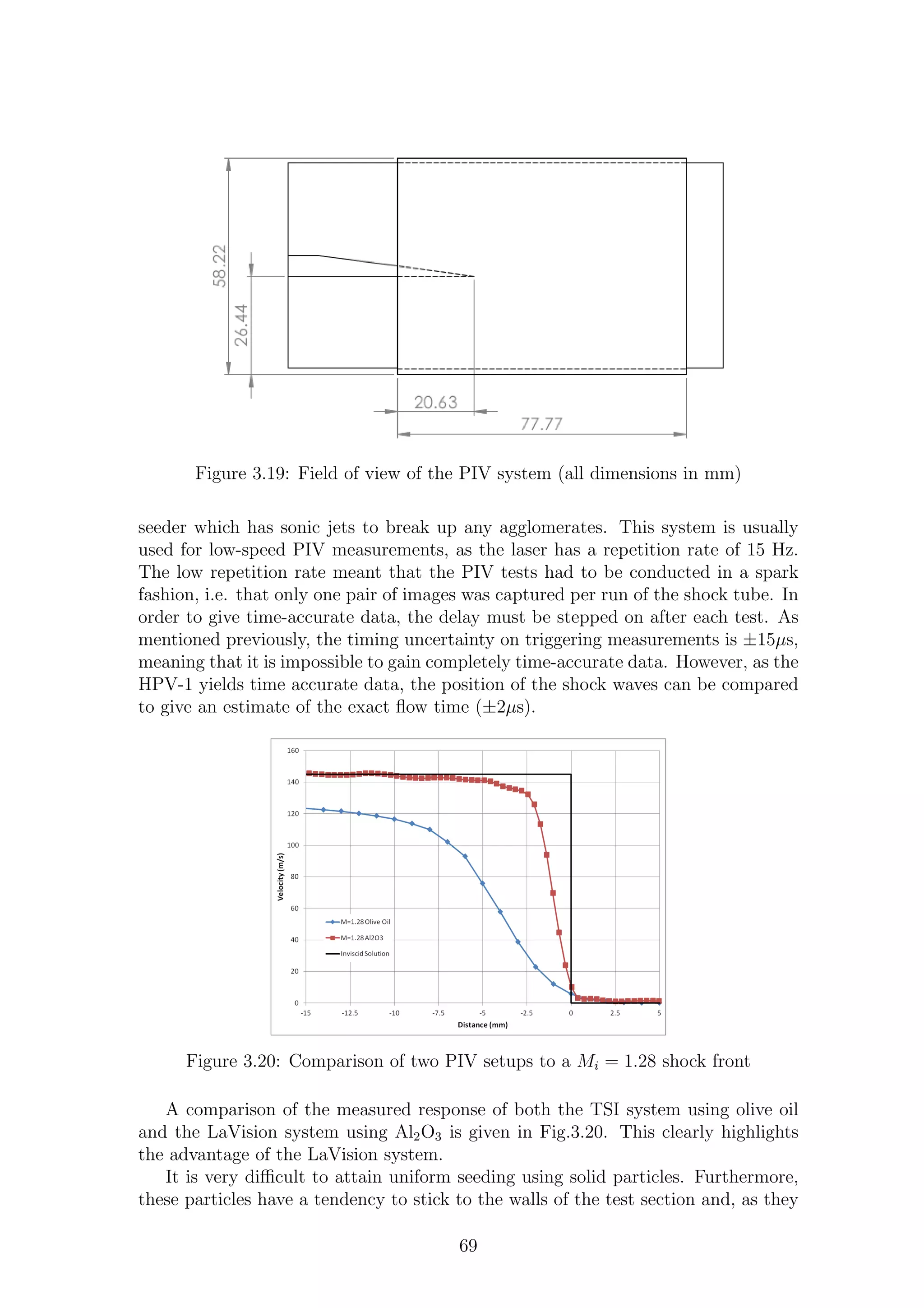
![are not transparent, block the signal from the laser sheet. This meant that after
every five runs, the shock tube had to be cleaned using anti-static screen wipes and
allowed to dry before testing could continue.
3.2.7 Post-Processing
The acquired raw PIV images were processed using LaVision’s Davis 7 software.
Initial coarse grids were refined using an iterative multi-grid method. The best
interrogation window was found to be 32 × 32 pixels (1.56 × 1.56 mm). When
combined with a 0.75 overlap factor between windows, this gives a vector plot of
150 × 200 vectors.
Post-processing of the velocity vectors was performed using Tecplot 2011. This
software allowed for the calculation of streamlines and vorticity magnitude. It was
found that the shock positions are most easily highlighted by calculating the ǫxy
component of the strain tensor.
ǫxy =
1
2
dU
dy
+
dV
dx
(3.29)
Statistical errors and the repeatability of the system were analysed using Tecplot
by extracting sub-zones of the whole data set around the region of interest.
3.2.8 Sources of Uncertainty
Measurement uncertainty and errors in PIV can be split into three main categories:
1. Errors associated with the camera and optical setup (signal measurement)
2. Errors associated with the tracer particle
3. Image/post-processing errors (signal analysis)
3.2.8.1 Signal Measurement Errors
The detection system used for PIV is usually a CCD camera. As a result of this,
most of the errors associated with CCD cameras apply to PIV, such as shot noise
etc.; however, these are usually negligible. If one particular pixel well on the CCD
is full, then a bleeding effect may occur, where the bloomed pixel spills over into
the pixel below it. Two-dimensional PIV is highly susceptible to large out-of-plane
velocity. The same is true of stereoscopic PIV if the laser sheet is not thick enough.
Incorrect scale calibration, as mentioned for density-based techniques, is another
possible source of error.
Errors caused by compressibility effects are harder to eliminate. The refractive
index of air changes with its density. As a result, if there are large density gradients,
such as in compressible flow for example, then optical aberrations can be caused
which blur the recorded image [142].
70](https://image.slidesharecdn.com/4a6f74b5-6bbb-4ffd-b3f5-7486cdb057cd-150303082443-conversion-gate01/75/Mark-Quinn-Thesis-101-2048.jpg)
![(a) P4/P1 = 4
(b) P4/P1 = 8
Figure 3.21: Shock front profile as measured by Al2O3 particles
3.2.8.2 Tracer Particle-Induced Errors
As mentioned in Section 3.2.3, tracer particles do not follow the flow precisely.
This can be a significant problem in compressible flow. The relaxation time causes
velocity lag which in turn creates spreading of the shock, often to several mm,
whereas in reality it is the same order as the mean free path length. A comparison
of the three pressure ratios used in this project is given in Fig.3.21. From these
figures it is clear that shock spread due to the tracer particle inertia is almost
constant for all of the Mach numbers being tested. Havermann et al. [124] showed
the curious phenomenon of a perceived velocity decrease upstream of a shockwave.
He ascribed this to the finite width of the interrogation region and the finite value of
∆t causing a predictive velocity drop. The effect of this can be reduced by altering
the size of the interrogation region accordingly.
Many researchers have encountered problems with measurements near the wall.
71](https://image.slidesharecdn.com/4a6f74b5-6bbb-4ffd-b3f5-7486cdb057cd-150303082443-conversion-gate01/75/Mark-Quinn-Thesis-102-2048.jpg)
![(c) P4/P1 = 12
Figure 3.21: Shock front profile as measured by Al2O3 particles
Schrijer et al. [122] cites direct light scattering from the solid wall, limited tracer
response and limited spatial resolution as possible reasons. This is often a problem
in thin boundary layers originating in high-speed flow, Mach 7 (1000m/s) in the
case of Schrijer et al. In order to counter this, other researchers (Humble et al.
[140]) allowed the boundary layer to develop over a 2m long plate, allowing it to
become ≈ 20mm thick. This thicker layer has longer scales associated with it and
is therefore easier to measure; however, this is not always possible due to length
constraints of experimental apparatus.
Based on the spread of the shock fronts displayed in Fig.3.21, it is estimated that
the nominal diameter of the tracer particles is approximately 0.5µm.
3.2.8.3 Signal Analysis Errors
Analysis of the images gained from PIV can contain errors associated with low
particle density, giving rise to so-called spurious vectors. This is often the case in
vortex cores where, as mentioned earlier (Section 3.2.3), particles tend to be ejected
due to the centrifugal forces involved. Fig.3.22 shows a raw PIV image of a vortex
ring emanating from a shock tube.4
The low level of data in these areas can often
give rise to large and clearly erroneous velocity vectors. Care must be taken not to
over-seed the flow in an effort to cure this problem, as saturation can also lead to
spurious vectors.
The most obvious factor that can be altered is the interrogation window size.
This will not only have the effect of producing more vectors but also of reducing
upstream velocity predictions [124]. This is only a valid option if there are enough
seeder particles in the fluid to fill each interrogation window. In such a transient
flow as this, it is virtually impossible to guarantee uniform seeding and, as such,
shrinking the interrogation window did not have any positive impact on the results.
4
Image reproduced with the permission of Dr. Raffaello Mariani
72](https://image.slidesharecdn.com/4a6f74b5-6bbb-4ffd-b3f5-7486cdb057cd-150303082443-conversion-gate01/75/Mark-Quinn-Thesis-103-2048.jpg)
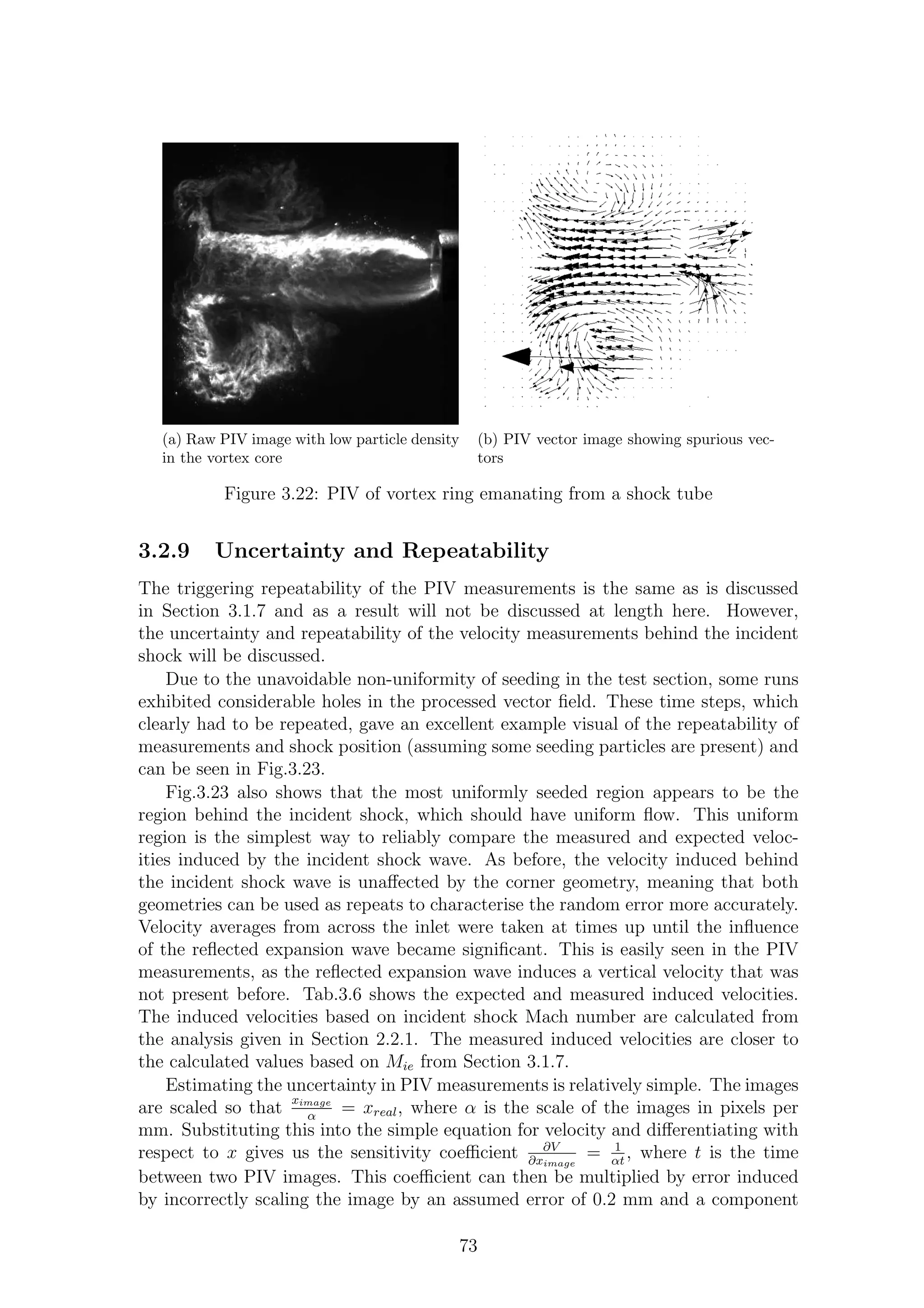
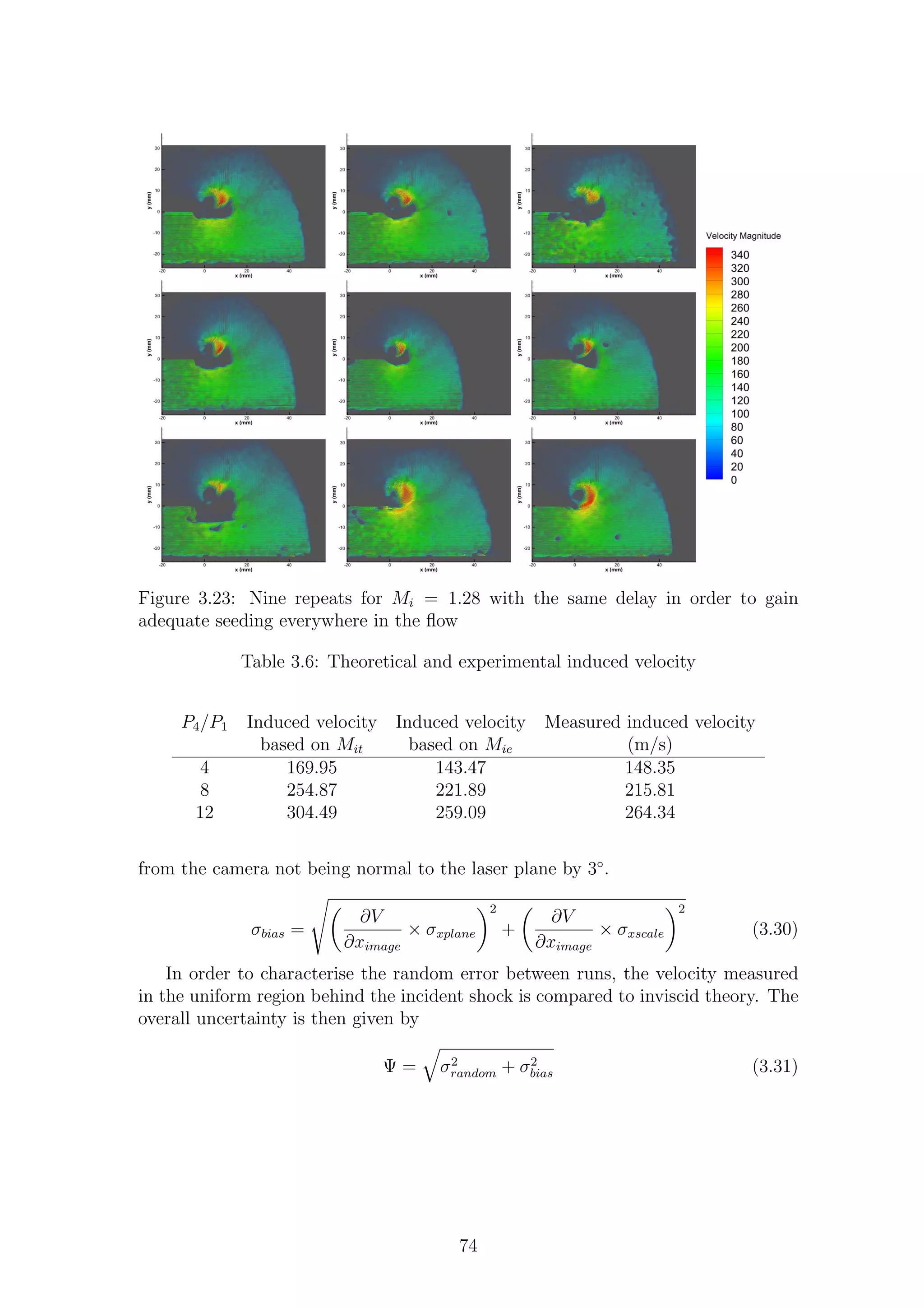
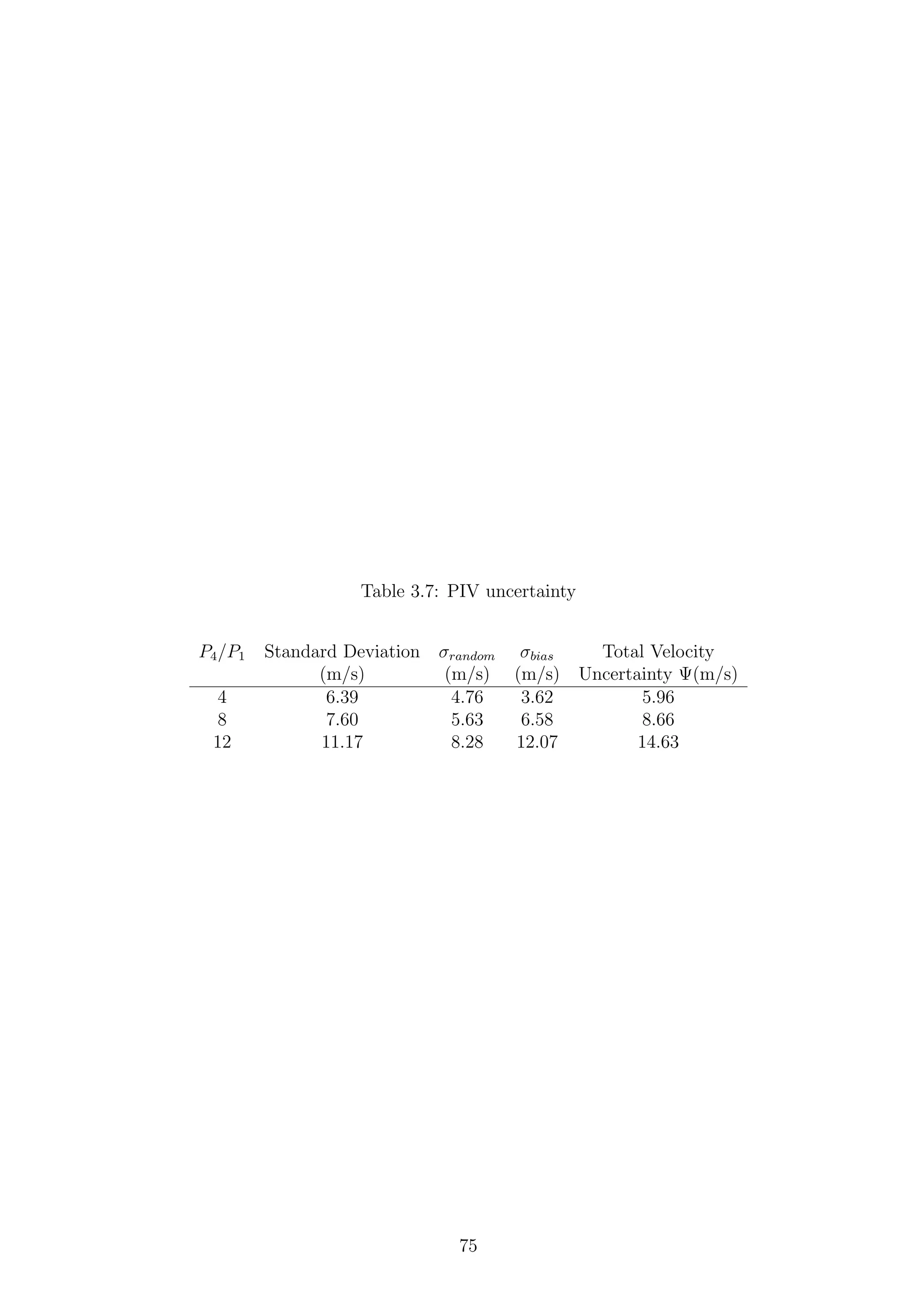
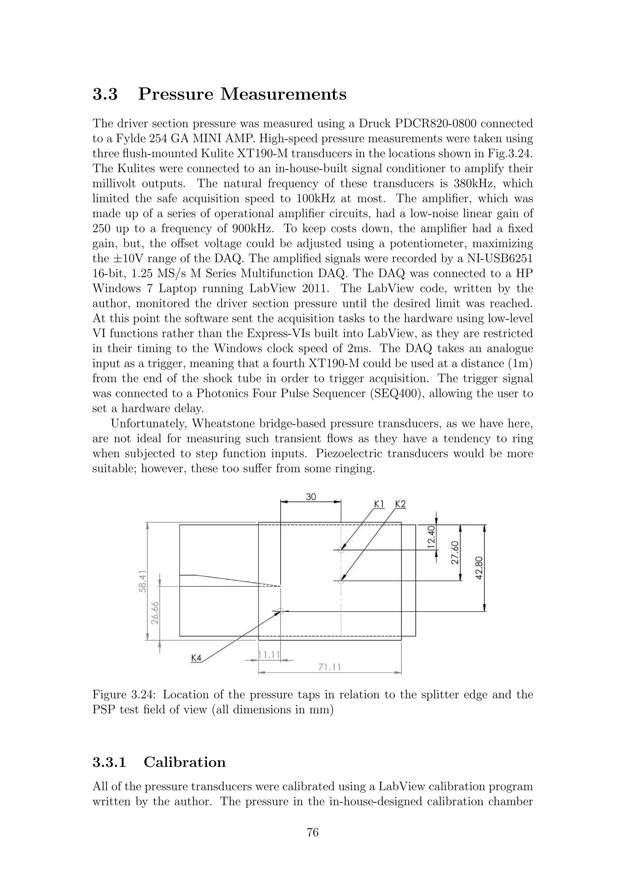
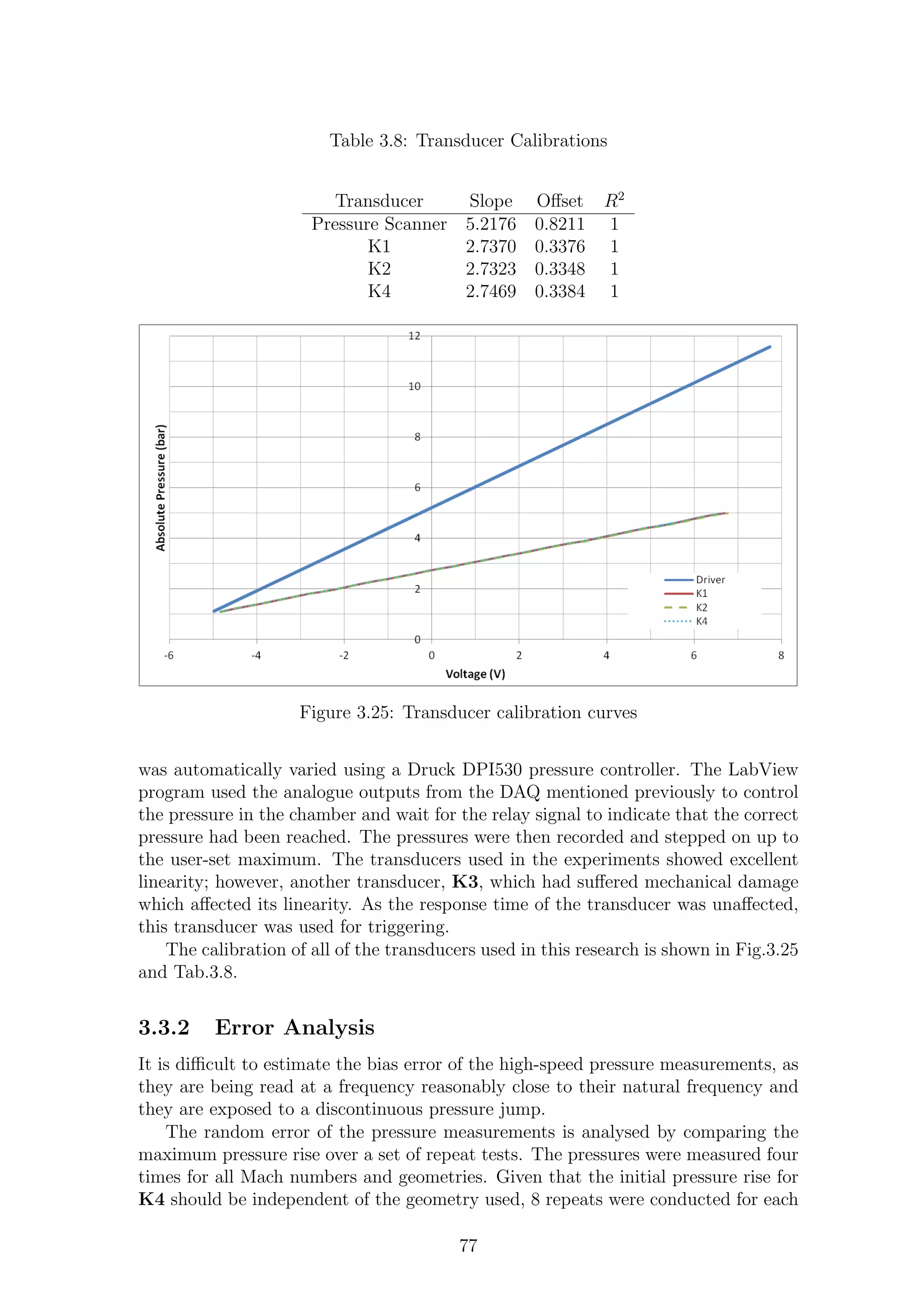
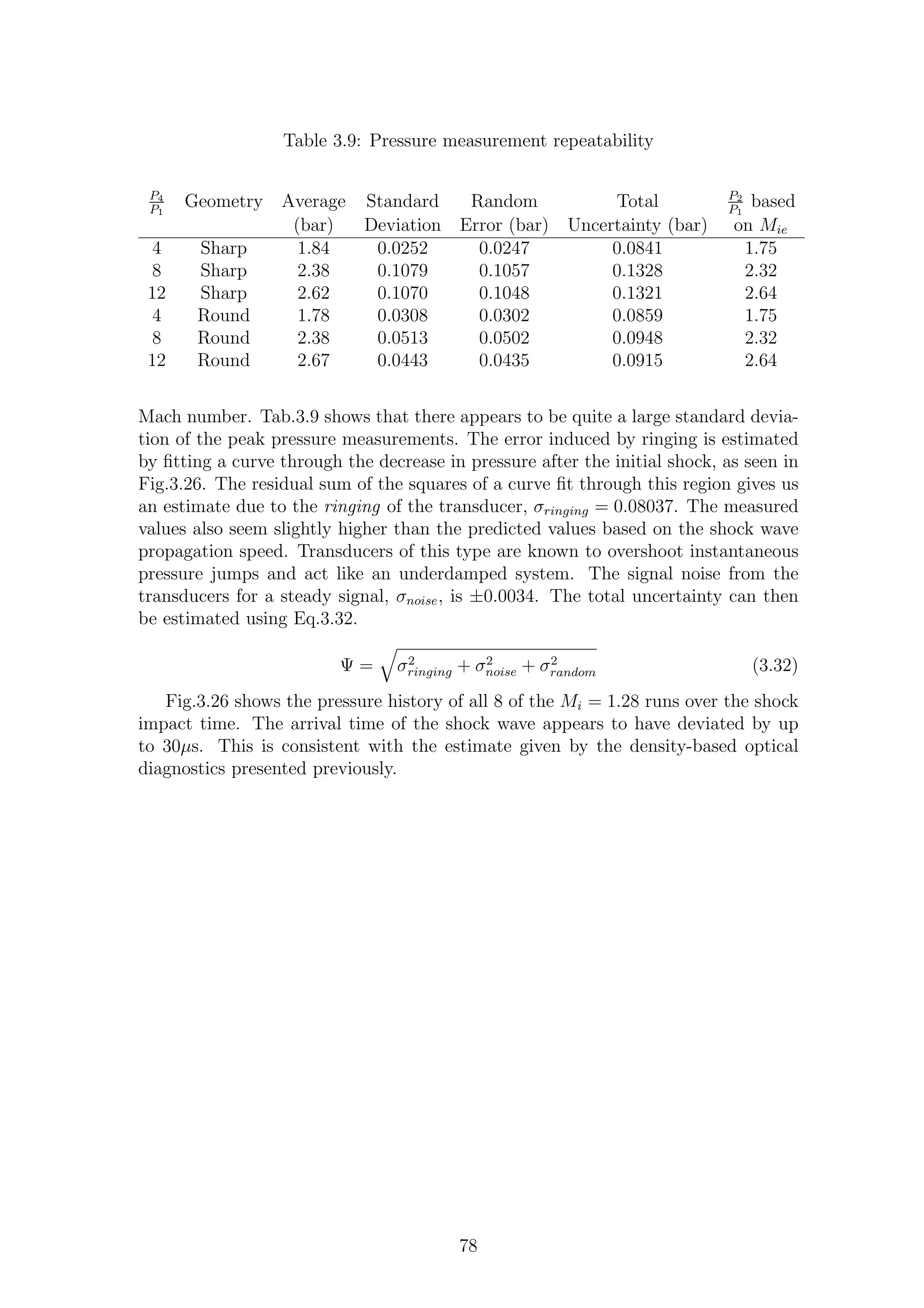
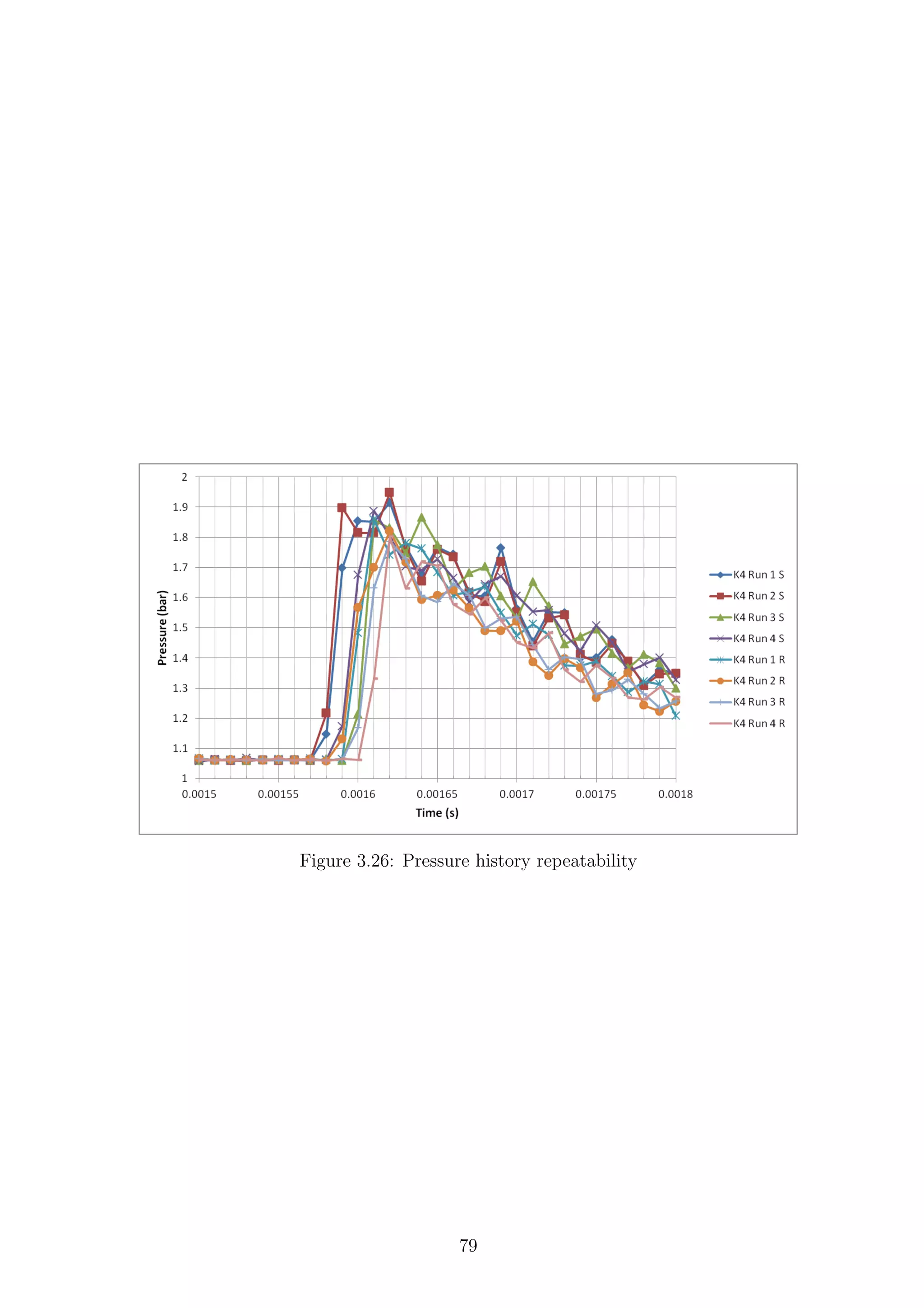
![3.4 Pressure-Sensitive Paints (PSP)
Although relatively still in its infancy, pressure-sensitive paint (PSP) is a useful
experimental tool for acquiring quantitative surface pressure measurements without
the need for a large number of pressure transducers. This method significantly
reduces the complexity of a model and can reduce the cost of creating a model too.
Installing many pressure transducers in a model is not only expensive and labour-
intensive but only gives discrete values of pressure, unlike PSP. Full surface pressure
maps can be achieved with PSP, as every pixel of an image can be regarded as a
pressure transducer. An excellent review of recent high-speed PSP (circa 2008) is
given by Gregory et al. [143].
3.4.1 History & Development
The origins of pressure-sensitive paint go back to the early 20th century and a
paper by Professor Max Volmer and Professor Otto Stern [144]. In this paper, the
researchers noted that luminescence of iodine vapour under the excitation of sunlight
was reduced by increasing pressure. This led them to a now famous relation bearing
their name. However, it took a further 16 years for the phenomena to be properly
understood. The German scientist Hans Kautsky discovered that the quenching of
luminescence was due to the presence of oxygen [145]. Kautsky adsorbed luminescent
compounds such as porphyrins onto silica gels and found a reciprocal relationship
between oxygen concentration and luminescent output. Soon after this work was
published, two independent streams of research on optical pressure sensors were
carried out on either side of the iron curtain. The two systems were developed in
Russia and the USA completely independently of each other, as is often the case
with scientific discoveries. The two teams remained completely unaware of each
other’s activities until an advertisement for the Russian system was published in the
February 12th
1990 edition of Aviation Weekly and was spotted by the American
team.
The American system evolved by chance from an idea by Dr. Martin Gouterman
to use luminescent molecules to sense the concentration of oxygen in blood. One of
Gouterman’s future PhD students, Prof. Jim Callis, had continued the research on
this topic and on the measurement of luminescent spectra. Prof. Jim Crowder, who
worked in the same building as Callis but on aerodynamic research, looked at ways
to improve the performance of the technique he championed, known as fluorescent
minitufts [146]. The collaboration between these two researchers and Gouterman
led them to apply luminescent coatings to the whole surface. This eventually led to
a transonic test of pressure-sensitive paint at NASA Ames [147], which showed the
feasibility of the technique and how it could be applied to whole surfaces. Kavandi
et al. [148] expanded on this work, showing the applicability of PSP and how it
could be used.
Meanwhile, Russian scientists at the the Central AeroHydrodynamic Institute
(TsAGI) had built on their own research of luminescent oxygen sensors [149] and
temperature-sensitive paints to design their own intensity-based pressure-sensitive
paint system. Wind-on and wind-off images and calibration techniques were pre-
sented by Aradsheva et al. [150]. This work led to the creation of a new research
team at TsAGI: the luminescent pressure sensor team. On this team was Prof.
80](https://image.slidesharecdn.com/4a6f74b5-6bbb-4ffd-b3f5-7486cdb057cd-150303082443-conversion-gate01/75/Mark-Quinn-Thesis-111-2048.jpg)
![Vladimir Mosharov, who was tasked with improving the system in use at TsAGI at
the time. The luminophore commonly used was acridine orange; a strange choice, as
it has an extremely low quantum yield (φ < 3%), requiring very high-power incident
lights to achieve a measurable signal. The polymer coating also had a long response
time (almost three minutes!). As this performance was improved over the follow-
ing years, an Italian firm (INTECO) reached an agreement to market the Russian
system to the West, leading to the aforementioned advertisement.
The Russian and American systems were very similar in specification and both
required significant improvement before they could be used reliably in transonic
tests and applied to different flow regimes. The vast majority of PSP tests have been
performed in steady transonic flow. These conditions give the largest pressure rise to
temperature rise and are therefore the easiest to measure. Low-speed measurements
are more challenging as PSP is an absolute pressure sensor, meaning that the changes
in absolute pressure can be very small. Unsteady PSP measurements have been
performed in a variety of ways, such as taking phase-locked point measurements
using photomultiplier tubes [151] or by introducing a different gas to change the
local partial pressure of oxygen [152].
3.4.2 Theory of PSP
There are two methods of utilising PSP: the lifetime and the intensity methods.
The intensity-based method will be discussed here, as it is in common use and is
currently the only method of PSP used at the University of Manchester. Lifetime
PSP systems involve significantly more complex and expensive setups. Despite this,
there are certain applications of PSP that can only be made using the lifetime
method (see Section 7.6).
Pressure-sensitive paints are based around the theory of oxygen quenching of
luminescence. This is closely related to, and often used in conjunction with, the
thermal quenching of luminescence, which is the basis of temperature-sensitive paint
(TSP). The photoactive molecule in the paint is called the luminophore and the
photophysics of this molecule is the basis for the PSP technique. Explained briefly,
an electron of a photoactive molecule absorbs a particular wavelength of light and
is excited from its ground state (S0) to a higher energy (singlet) state (S1 or S2).
The excited electron relaxes from higher vibrational states to the singlet level. The
electron can then relax to lower energy states by various methods, as shown by the
Jablonsky diagram (Fig.3.27). If the electron is in the S2 state, then by a method
called internal conversion, it can transfer to a vibrationally excited lower singlet
state by releasing some heat. The state S1 has many methods of returning to the
ground state which can be either radiative or radiationless. Radiative methods
involve fluorescence, i.e. the release of a photon. Radiationless methods include:
• Internal conversion: transfer to a vibrationally excited level of the ground state
followed by vibrational relaxation
• Intersystem crossing: transfer to a triplet excited state T1
• External conversion: contact with another molecule and transferring the en-
ergy to that molecule
81](https://image.slidesharecdn.com/4a6f74b5-6bbb-4ffd-b3f5-7486cdb057cd-150303082443-conversion-gate01/75/Mark-Quinn-Thesis-112-2048.jpg)
![Figure 3.27: Jablonsky energy level diagram
The triplet excited state, T1, can relax to the ground state by emitting a photon
of different wavelength to that emitted by the singlet state; this process is called
phosphorescence.5
Alternatively, the triplet state can relax to the ground state by
radiationless methods:
• Internal conversion: transfer to a vibrationally excited level of the ground state
followed by vibrational relaxation
• Intersystem crossing: transferring back to the singlet state S1, making all of
the above events possible again
• External conversion: contact with another molecule and transferring the en-
ergy to that molecule
The processes of fluorescence and phosphorescence are grouped together as ra-
diative processes and are usually referred to as luminescence [153]. As the processes
of fluorescence and phosphorescence have different lifetimes, they account for differ-
ent wavelengths of emission and cause spreading of the overall emission spectra (see
Fig.3.31).
The process knwon as external conversion is the basis of the PSP experimen-
tal method as the oxygen molecules in air remove the extra energy from the lu-
minophore, allowing it to return to its ground state. Oxygen molecules exhibit
excellent qualities as a quencher due to their unusual electronic ground state. The
oxygen molecules then return to their ground state by the methods presented above.6
Moreover, it should be noted that these oxygen molecules actually contribute to the
5
Fluorescence is the more useful form of radiation, as it takes place significantly faster (10−10
s)
than phosphorescence (10−3
s)
6
Oxygen does emit light but at a much higher wavelength, mid infra-red (λ > 1240nm)[154]
82](https://image.slidesharecdn.com/4a6f74b5-6bbb-4ffd-b3f5-7486cdb057cd-150303082443-conversion-gate01/75/Mark-Quinn-Thesis-113-2048.jpg)
![degradation of the paint. The excited oxygen molecule is highly reactive and can
bind irreversibly with the paint surface, causing it to lose its photoactive properties.
Clearly, there are different ways in which an excited molecule can return to its
ground state: radiative processes Kr, non-radiative processes Knr or by quenching
Kq. The quantum yield (φ) is the ratio of luminescence to excitation and is a measure
of the efficiency of a paint.
φ =
luminescence
excitation
=
Kr [L∗
]
Ia
=
Kr
Kr + Knr + Kq [Q]
(3.33)
where L∗
is an excited luminophore, Ia is the incident light absorbed, Q is the
quencher and all brackets enclosed in square brackets [ ] denote concentration. If
we now consider the response of the paint in a vacuum we arrive at the quantum
yield without any quenching:
φ0 =
Kr
Kr + Knr
=
I0
Ia
(3.34)
noting that I0 is the emission in a vacuum and, in general, symbols with a
subscript 0 denote vacuum conditions. Now taking the ratio of the quantum yields
with and without quenching:
φ0
φ
=
Kr
Kr+Knr
Kr
Kr+Knr+Kq[Q]
=
Kr + Knr + Kq [Q]
Kr + Knr
= 1 +
Kq
Kr + Knr
[Q] = 1 + Kqτ0 [Q]
(3.35)
Equation (3.35) is the initial form of the widely recognised Stern-Volmer equa-
tion. This equation can reduce to give the luminescent lifetime τ with and without
quenching depending on whether or not quenching is included:
τ0 =
1
Kr + Knr
(3.36)
τ =
1
Kr + Knr + Kq [Q]
(3.37)
This means that the Stern-Volmer equation (3.35) can be written as:
φ0
φ
=
I0
I
= 1 + Kqτ0 [Q] =
τ0
τ
(3.38)
As mentioned above, oxygen is an excellent quencher and is the quencher that
is of use here. With this in mind, we can replace [Q] with [O2].
The rate constants Knr and Kq are temperature-dependent. It is this temper-
ature dependency that is the main flaw of almost all PSP measurements. Non-
radiative processes can be modelled by the Arrhenius relationship and broken down
into temperature-dependent and temperature-independent terms.
Knr = Knr0 + Knr1 e
−
EAnr
ℜT
(3.39)
where EAnr is the activation energy of the reaction, ℜ is the universal gas con-
stant, Knr0 is the temperature-independent, non-radiative process and Knr1 is the
83](https://image.slidesharecdn.com/4a6f74b5-6bbb-4ffd-b3f5-7486cdb057cd-150303082443-conversion-gate01/75/Mark-Quinn-Thesis-114-2048.jpg)
![temperature-dependent, non-radiative process.
From this point onwards in the derivation of PSP, the exact format of the models
used is dependent on the substrate and the application method, whether polymer-
based or porous. This will be covered in Section 3.4.3. However, for now we will
treat polymer-based PSP first and then extend this to include porous-based PSP.
The temperature-dependency of the quenching rate is due to the diffusion of
the quenching molecules through the polymer layer7
. This can be modelled by the
Smoluchowski relationship, where the rate of quenching can be expressed as:
Kq = 4πRABN0D (3.40)
where RAB is an interaction distance, N0 is Avogadro’s number and D is the
diffusivity. The diffusivity is the term which is dependent on temperature; all of
the others are constants for a given system. Kinetic theory dictates that the kinetic
energy of a molecule is dependent on the cube of temperature. If the temperature
increases then the increase in kinetic energy increases the frequency of collisions
between the luminophores and O2 molecules. This increased frequency of collisions
makes it more likely that the excited luminophore will be deactivated by external
conversion (quenched). The diffusivity of the quencher through the polymer can be
modelled by the Arrhenius relationship.
D = D0e
−
EAD
ℜT
(3.41)
where EAD
is the activation energy required for diffusion. Equations 3.39, 3.40
and 3.41 can be substituted into equation 3.37 to give:
1
τ
= Kr+Knr+Kq [Q] = Kr+Knr0 +Knr1 e
−
EAnr
ℜT
+4πRABN0D0e
−
EAD
ℜT
[O2]polymer
(3.42)
Henry’s Law states that, at constant temperature, the amount of gas dissolved
in a solid is proportional to the gas pressure at the surface. This means that the
amount of oxygen in the polymer layer is related to the partial pressure of oxygen by
a solubility constant, S. From Dalton’s law of partial pressures, the total pressure
of the gas (P) multiplied by the molar fraction of oxygen (χO2 ) gives us the partial
pressure of oxygen. This means that Equation 3.42 can be written in the form:
1
τ
= Kr + Knr0 + Knr1 e
−
EAnr
ℜT
+ 4πRABN0D0e
−
EAD
ℜT
SPχO2 (3.43)
Previously, the ratio of intensity with and without quenching was shown. As
mentioned before, the only condition in which no quenching will occur is in a vacuum
(or oxygen-free environment). In order to generate a more practical expression
7
The increased temperature gives the molecules more kinetic energy, which increases the diffu-
sion rate. Although a porous PSP setup involves no diffusion through a polymer layer, the same
increase in quenching is observed. This is related to the increased kinetic activity of the quenching
molecules and is accounted for in the equation, as many of the constants drop out leaving only
temperature ratios.
84](https://image.slidesharecdn.com/4a6f74b5-6bbb-4ffd-b3f5-7486cdb057cd-150303082443-conversion-gate01/75/Mark-Quinn-Thesis-115-2048.jpg)
![(rather than referencing to a vacuum), Equation 3.43 is evaluated at any arbitrary
condition and divided by Equation 3.43 at a reference condition.
τref
τ
=
Iref
I
=
Kr + Knr0 + Knr1 e
−
EAnr
ℜT
Kr + Knr0 + Knr1 e
−
EAnr
ℜTref
+
4πRABN0D0e
−
EAD
ℜT
SPχO2
4πRABN0D0e
−
EAD
ℜTref
SPref χO2 ref
(3.44)
Assuming that the only variables that change are pressure and temperature
between the two conditions and assuming that the temperature change is not signif-
icant enough to cause species change in the gas and therefore a change in the molar
fraction of diatomic oxygen, Equation (3.44) can be reduced to give:
Iref
I
= A(T) + B(T)
P
Pref
(3.45)
Equation 3.45 is a modified form of the Stern-Volmer relationship and has the ad-
vantage that, when practically applied to an image of a painted surface, any surface
non-uniformities are theoretically eliminated. This can be extended by considering
the method of contact between luminophore and quencher.
If we assume that the oxygen concentration adsorbed on to the surface can be
modelled by a fraction of the coverage of the surface:
Θ =
[O2]ads
[O2]adsMax
(3.46)
where [O2]adsMax is the maximum oxygen concentration on the surface, we can
write Equation 3.35 as
I0
I
= 1 + Kqτ0 [O2]adsMax Θ (3.47)
leading to
Iref
I
= A(T) + B(T)
Θ
Θref
(3.48)
Sakaue [155] showed that the Freundlich isotherm (Equation 3.49) can be used
as a model for the surface adsorption of oxygen onto the substrate, as it is a model
of the amount of occupied adsorption sites compared to the total number of possible
sites.
Θ = bf (PO2 )γ
(3.49)
The constant bf is a function of temperature and activation energy (also a func-
tion of temperature) and γ is an empirical constant to be experimentally determined
for every system. Substituting Equation 3.49 into Equation 3.48 gives:
Iref
I
= AFreundlich(T) + BFreundlich(T)
PO2
PO2ref
γ
(3.50)
If PSP measurements are required over very large pressure ranges, Equation 3.45
85](https://image.slidesharecdn.com/4a6f74b5-6bbb-4ffd-b3f5-7486cdb057cd-150303082443-conversion-gate01/75/Mark-Quinn-Thesis-116-2048.jpg)
![does not model the non-linear behavior of the PSP well and it is more useful to use
Equation 3.50, as the constant, γ, accounts for the non-linearity. This was shown
experimentally by the author [156].
The exact format of the constants AFreundlich & BFreundlich is not important as
they are determined by proper calibration. Naturally, it would be more helpful if
they were weak functions of temperature; however, this is not just dependent on the
substrate but also a function of the combination of the substrate and luminophore.
3.4.3 PSP Substrates
The substrate of a PSP determines some of its most important characteristics, such
as the response time and the sensitivity range. Temperature sensitivity, signal out-
put and, occasionally, spectral performance, can also be affected. The choice of an
appropriate substrate is one of the most important decisions in the design of any
PSP experiment and was the subject of a recent study by the author [156].
There are two main types of PSP substrate and a variety of hybrids of the two.
The main choice is between either a permeable or a porous substrate. Permeable
substrates commonly consist of a polymer layer which is highly permeable to oxy-
gen. The luminophore is suspended in this oxygen-permeable layer, allowing it to be
deactivated by oxygen which has diffused into the layer. The application of a reflec-
tive basecoat increases the adhesive properties of the active layer but also reflects
more light towards the imaging device, increasing the measurable signal (Fig.3.28a).
The polymers used at the University of Manchester are known as sol-gels. The
sol-gel method is relatively cheap and very easy to perform, requiring very little
expensive equipment and has been shown to give excellent results [157]. B. J. Basu
[158] showed that the sol-gel films have excellent optical and mechanical properties
when applied properly and also showed that the porosity, as well as other properties,
of the sol-gel matrix layer can be tailored to suit. MacCraith & McDonagh [159]
showed the versatility of sol-gel layers and how their chemical composition has a
large impact on the response of the luminophore (or flurophore, as they called it).
The sol-gel layer can develop cracks after it has been cured, due to the sol-gel matrix
reducing in volume as the solvent (ethanol in many cases) is evaporated off.
Tab 3.10 shows the typical response time of some polymer-based PSP tests.
Clearly, for this project such a slow response time is unacceptable and faster al-
ternatives must be considered. The limit on the response time of polymer-based
PSP is the diffusion time through the polymer layer [153]. In order to remove this
limit, several researchers have developed the use of porous substrates where the lu-
minophore is adsorbed onto the surface, meaning that it is in direct contact with
the test gas (Fig.3.28b).
Baron et al. [160] compared the response times between porous and polymer-
based oxygen-sensing coatings. This study paved the way for porous substrates to
be developed by other researchers, as it showed that the response time could easily
be sub-millisecond.
There are two common porous substrates used in high-speed PSP testing: Thin
Layer Chromatography (TLC) plates and anodised aluminium. TLC plates are
highly adsorbent and have an excellent response time. The work by Baron et al.
[160] illustrated that a porous TLC PSP setup could be used to give very fast
response times (10s of microseconds). Sakamura et al. [161] showed that a TLC
86](https://image.slidesharecdn.com/4a6f74b5-6bbb-4ffd-b3f5-7486cdb057cd-150303082443-conversion-gate01/75/Mark-Quinn-Thesis-117-2048.jpg)
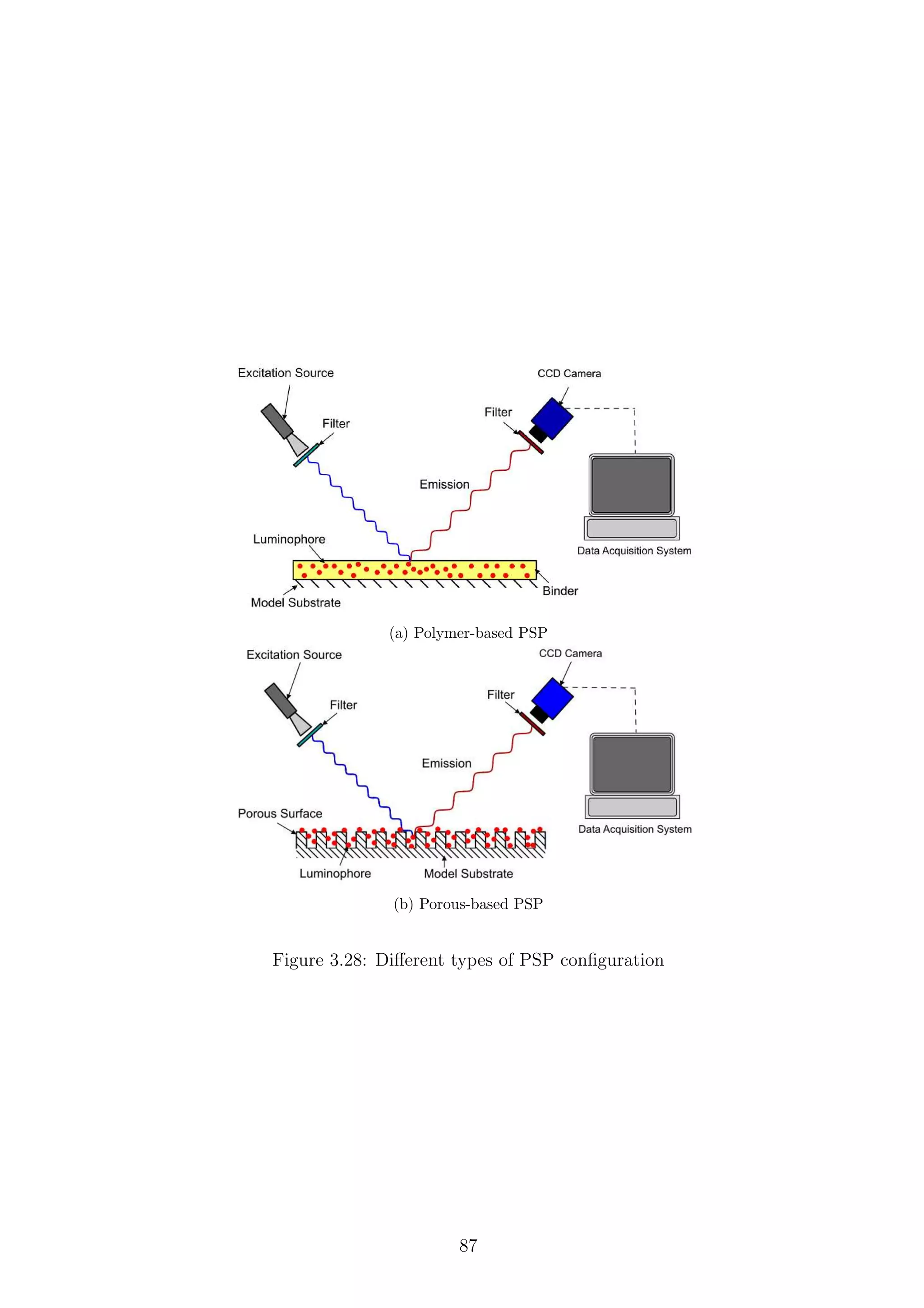
![Figure 3.29: Mechanical damage to several initial TLC plates after 10 runs of the
shock tube
plate could be used to show transient shock wave phenomena such as the movement
of starting shocks in supersonic nozzles, almost impossible to achieve with a finite
number of pressure transducers. TLC plates are cheap to buy and it is very easy to
apply the luminophore to the surface. However, the plates themselves are extremely
brittle and can easily be subject to mechanical damage. As a result of this, they are
usually applied only to simple geometries [162] and often have to be replaced due
to cracking or fracturing. An example of this can be seen in Fig.3.29.
Anodised aluminium was first suggested as a suitable porous matrix material
by Mosharov et al. [163]. A comparison of various matrix materials and binding
methods was performed by Sakaue & Sullivan [164], which showed that anodised alu-
minium gives response times that are fast enough to capture high-speed unsteady
phenomenon such as moving shock waves. The speed of this response, as shown by
Kameda et al. [165] and Hangai et al. [166], is determined by both the pore diam-
eter and depth. It was shown that the anodisation process (voltages, electrolytes
and length of time) has a large effect on the pore size and depth. The most effec-
tive combination appears to be the shallowest and widest pores, as these have the
fastest response time. The author has shown [156] that the signal level given by
luminophores adsorbed onto anodised aluminium is far too low to measure at high
speed using a single shot approach.
So far we have encountered a porous substrate which can only be used on simple
flat surfaces and one which can only be used on aluminium. There is a hybrid of
these two types of substrates where a porous substrate can be sprayed on to any
surface. This is known as the polymer ceramic method. Of the limited literature
available on this method ([143],[167],[168],[169],[170]), it has been shown that the
response time appears to be 25µs minimum. In a similar way to polymer-based PSP,
this is dependent on the thickness of the coat [143] and the polymer content [170].
The response time of different PSP substrates is given in Tab.3.10. Many more
researchers have shown similar response times; however, these cover the typical
range. Several different values given in the research of Sakaue [164] [171] [172] show
variation of solvents and of pore depth. A more detailed discussion on this topic is
given in the review by Gregory et al. [143].
88](https://image.slidesharecdn.com/4a6f74b5-6bbb-4ffd-b3f5-7486cdb057cd-150303082443-conversion-gate01/75/Mark-Quinn-Thesis-119-2048.jpg)
![Table 3.10: Response time of PSP substrates
Substrate Test type 90% response time Author
[ms]
Silica gel Solenoid valve 10 Baron et al. [160]
Silica gel Solenoid valve 1.5 Baron et al. [160]
Polymer Solenoid valve 480-2500 Carroll et al. [173]
Polymer Shock tube 3-6 Hubner et al. [174]
Polymer Shock tube 172 Sakaue & Sullivan [164]
Sol-gel Solenoid valve 5-540 McDonagh et al. [175]
Anodised aluminium Shock tube 0.035-0.102 Sakaue & Sullivan [164]
Anodised aluminium Shock tube 0.03-0.04 Sakaue [171]
Anodised aluminium Shock tube 0.06 Kameda et al. [176]
Anodised aluminium Shock tube 0.05-0.15 Sakaue et al. [172]
TLC Solenoid valve 0.025 Baron et al. [160]
TLC Shock tube 0.065 Sakaue & Sullivan [164]
TLC Shock tube 0.04 Sakamura et al. [161]
TLC Shock tube 0.15 Hayashi et al. [169]
Polymer ceramic Shock tube 0.349 Sakaue & Sullivan [164]
Polymer ceramic Shock tube 0.15 Hayashi et al. [169]
3.4.4 Luminescent Compounds
Optical pressure measurements are only possible using compounds which display
sensitivity to the gas used (in our case oxygen). There are many luminophores
that exhibit different properties, such as pressure and temperature sensitivity, quan-
tum yield, luminescent lifetime and photodegradation. The review by Takeuchi &
Amao [177] gives an excellent overview of the photoactive compounds which are
currently in use. They are largely broken down into three categories: transition
metal polypyridyl complexes, porphyrins and polyaromatic hydrocarbons. With the
exception of polyaromatic hydrocarbons, these complexes are extremely difficult to
synthesise and, as such, can be very expensive.
Only Ru(dpp)2+
3 (or, to give it its full name, tris-Bathophenanthroline Ruthenium
II Perchlorate) will be covered in detail in this review. The other two luminophores
considered, PtTFPP and PBA, have problems associated with this kind of test which
prohibited their use (namely, PtTFPP has too long of a luminescent lifetime to gain
meaningful results; and PBA has very high photodegradation [178] and it is difficult
to illuminate it with the required power in its absorption range).
Ru(dpp)2+
3 (Fig.3.30) has excellent properties as a luminophore, such as a high
quantum yield, excellent pressure sensitivity and acceptable temperature sensitivity
[156]. The molecule has also been shown to be highly photostable, meaning that it
can be used in repeat tests. It also exhibits a large Stokes shift [179], a desirable
property of any photoactive molecule. This large Stokes shift can be seen in Fig.3.31
as the large gap between the excitation and emission signals. The luminescent
lifetime of Ru(dpp)2+
3 is approximately 5µs [180], which sets the ultimate limit on
the luminophore response time. Other luminophores have much shorter lifetimes
89](https://image.slidesharecdn.com/4a6f74b5-6bbb-4ffd-b3f5-7486cdb057cd-150303082443-conversion-gate01/75/Mark-Quinn-Thesis-120-2048.jpg)
![(PBA, for example); however, Ru(dpp)2+
3 is the best all-round luminophore, which
explains why it is the most commonly used.
Figure 3.30: Ru(dpp)2+
3 molecule
Figure 3.31: Excitation and emission spectra of Ru(II) and PtTFPP[4]
3.4.5 Limitations
There are several limitations of PSP which affect its application to all flow speeds.
Low-speed limitations have been covered by the author in other works [156][181][182].
Consequently, only high-speed limitations will be covered in this section.
As with all PSP measurements, the temperature-induced error is often the largest
source of error. This has been a major problem in the application of PSP to high-
speed flow, as large changes in static temperature are expected. This has led some
researchers to use different calibrations on either side of a shock wave to account
for the temperature change [148][183]. The author has shown that the temperature
dependency of the PSP formulations typically used at the University of Manchester
[156] is typically −0.9%◦
C−1
. This is a significant problem for the measurement
of steady and quasi-steady flows. However, the flow under investigation in this
project is transient; as such, the temperature change over the model is expected to
be negligible.8
8
Estimates using the thermal conductivity properties of aluminium gave temperature changes
of less than 0.01◦
C over 250µs.
90](https://image.slidesharecdn.com/4a6f74b5-6bbb-4ffd-b3f5-7486cdb057cd-150303082443-conversion-gate01/75/Mark-Quinn-Thesis-121-2048.jpg)
![Over time, and under illumination, PSP will photodegrade, become less sensitive
to oxygen and give out a lower signal output. The mechanisms of this were the focus
of a study by Egami & Asai [178]. The use of powerful light sources for excitation
only exacerbates this problem. Photodegradation rates of 4.5% per hour are typical
for low-level excitation [156]; however, for this research, the use of a much more
powerful light source means that this value could be significantly higher. Despite
this, the total acquisition time for this project is only of the order of milliseconds,
meaning that photodegradation can be neglected (provided that in-situ calibration
is used).
Gregory et al. [184] showed the difference in response between an increase and a
decrease in pressure. Their results showed that decreases in pressure were displayed
in the PSP results more quickly than increases in pressure. They showed the varia-
tion of these changes for different constant values of Equation (3.50). It was found
that the response times became closer as the exponent, γ, decreased.
Porous substrates readily adsorb water from the test gas onto the surface. This
can have a significant effect on the sensitivity and luminescent output of the samples
[176] (up to a 10% change in intensity output from dry air to 50% relative humidity).
To this end, Sakaue et al. [172] developed a hyrdophobic coating to apply to porous
PSP in order to reduce its sensitivity to changes in humidity. Due to the sensitivity
of the PSP to humidity, all of the TLC samples created were baked in an oven to
reduce their local moisture content before testing.
Due to the extremely short exposure time required to accurately capture tran-
sient flows, acquiring a measurable signal can be a significant problem. One cannot
simply increase the luminophore concentration, as this will affect the sensitivity
and can actually reduce the signal output [185]. Therefore, the only viable alterna-
tives are to use very powerful light sources and highly sensitive cameras. In some
high-speed experiments [176][172], laser light sources have been used. This has the
advantage of guaranteeing that there is no spectral leakage between excitation and
emission, but also has the problem of not utilising the whole excitation spectrum
of the luminophore. Therefore, broadband light sources can be used in conjunction
with filters. Using high-power broadband light sources increases risks to safety, with
high levels of UV radiation emitted.9
The heat generated by these light sources
needs to be removed, ideally by using a water filter; however, this is sometimes
not enough to prevent damage to other components in the optical train. It is the
recommendation of the author that any experimentalist wishing to conduct tests of
this nature do so using filters based on reflectance rather than absorption. Despite
taking every possible cooling precaution when using absorption-based filters, they
are still likely to break due to the thermal stresses created by the beam (see Fig.3.32
for an example10
).
9
High-power light sources also give rise to the creation of O-zone, another potential health
hazard.
10
The same fate was met by other filters, including heat-proof glass used for IR absorbance.
91](https://image.slidesharecdn.com/4a6f74b5-6bbb-4ffd-b3f5-7486cdb057cd-150303082443-conversion-gate01/75/Mark-Quinn-Thesis-122-2048.jpg)
![Figure 3.32: The fate of a UG5 400 nm short-pass filter after 20 seconds’ exposure
to a 1 kW beam after a water and blue dichroic filters
3.4.6 Applications
Pressure-sensitive paints have been used in wind tunnels of almost all speeds from
low-speed automobile testing up to hypersonic vehicle design. The range of pressure
changes that they can reliably detect is always on the increase and appears to be
a function of the imaging system used. Engler et al. [186] captured a resolution of
500 Pa using a lifetime-based method and managed to successfully resolve leading-
edge vortex roll-up on a delta wing at Mach 0.9 using an intensity-based system.
It was shown by McGraw et al. [187] that pressure changes as low as 6 Pa can be
detected in a resonant cylinder, allowing the PSP sample to effectively be used as
a microphone. McGraw et al. [151] and Nakakita [188] both showed resolutions
of ≈ 200 Pa for vortex shedding from two-dimensional objects at a frequency of
95 − 125 and 2000 Hz respectively. Nakakita utilised a very interesting and novel
data analysis technique based on the Fast Fourier Transform (FFT) which showed
the importance of different parts of the frequency range of vortex shedding allowing
for accurate calculation of the Strouhal number. Henne [189] showed a resolution
of 150 Pa on measurements of an A400m half model at low speeds. This research
incorporated active temperature correction by using an infra-red imaging device.
The author has used PSP to capture the flow around a U-bend used to model the
flow around the cooling passages found in turbine blades [181][182].
The advent of porous PSP has meant that it became possible to use PSP in cryo-
genic applications, as no oxygen diffusion is needed (it is usually hindered/prevented
by a polymer layer at such low temperatures [190]).
Practical applications of PSP have been shown by numerous researchers: Klein
et al. [191], Zare-Behtash et al. [192], Engler et al. [193] [186] and Sakamura &
Suzuki [194], to name just a few. Klein et al. [191] showed that PSP can be used
to calculate normal forces and moments on model aircraft in wind tunnel tests.
Although force balances are an excellent way of measuring this and do not usually
need to be replaced, the comparison shows that surface integration of PSP tests
92](https://image.slidesharecdn.com/4a6f74b5-6bbb-4ffd-b3f5-7486cdb057cd-150303082443-conversion-gate01/75/Mark-Quinn-Thesis-123-2048.jpg)
![can yield accurate results ±5%. Sakamura & Suzuki [194] showed that the starting
shock of a de-Laval nozzle can be captured using a porous PSP setup and a high-
speed CMOS camera. This body of research highlights the potential that PSP has
for imaging transient phenomena, leading to almost limitless applications within the
aerospace research or design sectors. Non-engineering applications of PSP, or rather
oxygen sensitive luminophores, have also been demonstrated. Mills [195] and other
researchers have used luminescent complexes to measure the oxygen levels of blood
samples.
3.4.7 Setup
The high-speed PSP system used in this research is shown in Fig.3.33. Two blue
dichroic filters purchased from Edmund optics, used in conjunction with heat ab-
sorbent glass, were placed in front of the excitation light source (consisting of 1000
W and 300 W xenon arc lamps, providing broadband excitation). Both xenon arc
lamps were purchased from Newport Oriel. The 1000 W lamp requires a water filter,
which was powered using an in-house-constructed water filter system. The emission
signal was filtered using a 530 nm long-pass filter attached to a Vision Research
Phantom 710 high-speed video camera. The spectra of the light source and the
relevant filter transmissions were measured using the Princeton Instruments ICCD
spectrometer and are given in Fig.3.34. The Phantom camera is well-suited to tests
of this type due to its large pixel size and high quantum efficiency over a wide range
of wavelengths. The capture rate is 100 kHz with an exposure time of 9.6µs. At
such a high frame rate, the image resolution was limited to 224 × 184 pixels giving
a pixel density of approximately 3.2 pixels per mm. The field of view of the PSP
experiment is shown in Fig.3.24. The images were stored on a PC running Win-
dows XP using Vision Research’s proprietary software. Triggering of the capture
as performed using the same Kulite transducer as the previous tests without the
delay generator. The decision not to use a delay generator was taken so that the
images taken before the arrival of the shock wave could be averaged and used as the
reference, wind-off image.
3.4.7.1 Sample Preparation
In order to deposit some luminophore onto a surface, it first must be dissolved
in solution. Sakaue [171] showed the difference between ten solvents with widely
varying polarity. It was found that some non-polar solvents would not dissolve even
a small amount of the luminophore (this is especially a problem for PBA). The two
most promising solvents for dissolving Ru(dpp)2+
3 are dichloromethane and acetone,
as these deposited the most luminophore on the surface, therefore producing the
highest signal level. Dichloromethane gave the highest pressure sensitivity over a
large range; however, acetone gave the highest signal output.
It is known that the higher the concentration of luminophore in solution, the
more will be deposited on the surface, until the surface is saturated. However,
Sakaue & Ishii [185] showed that increasing the amount of luminophore deposited
on the surface does not monotonically increase the signal output or the sensitivity;
rather, it decreases past a critical value. They found that the optimum luminophore
concentration is of the order of 0.1 mM. Sakaue & Ishii [196] also showed that the
93](https://image.slidesharecdn.com/4a6f74b5-6bbb-4ffd-b3f5-7486cdb057cd-150303082443-conversion-gate01/75/Mark-Quinn-Thesis-124-2048.jpg)
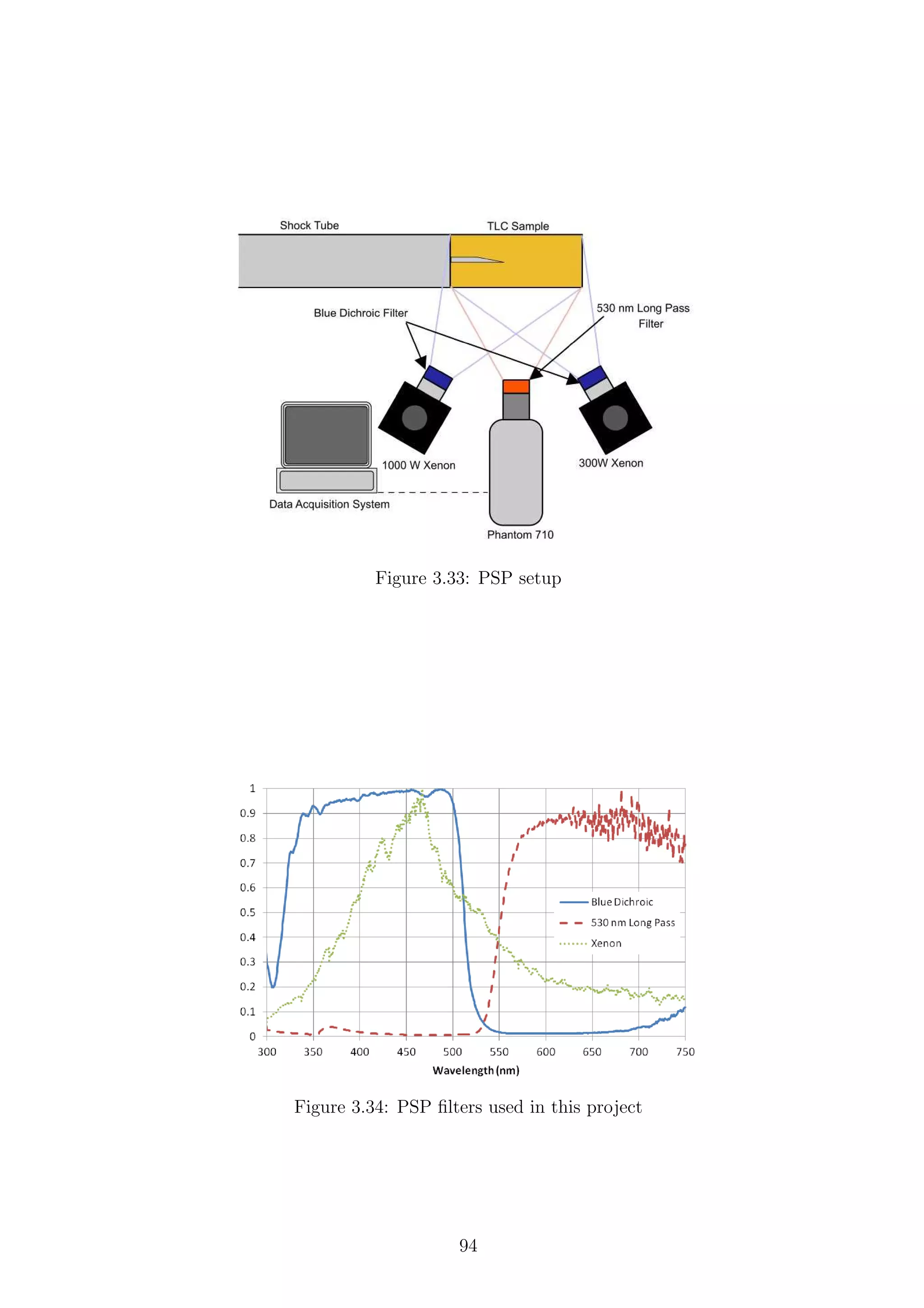
![length of time for which the substrate is immersed in the luminophore solution has
a strong effect on the signal output and the temperature sensitivity of the final
sample. They found the optimum time to be approximately 17 minutes.
Using the two basic formulae related to molar concentrations allows for the cal-
culation of the required mass of luminophore in a given volume of solvent for a
specific concentration. 64.85 mg of Ru(dpp)2+
3 (purchased from GFS chemicals) was
dissolved in 100 ml of dichloromethane (purchased from Sigma Aldrich) at room
temperature, giving a 0.5 mM solution.11
The TLC plate (MERCK HPTLC Silica-
Gel 60) has been used previously by Gongora-Orozco et al. [197], who showed the
difficulties which can occur using the dipping method of application. If great care
is taken, uniform application can be achieved using this method, as can be seen in
Fig.3.29. The samples were placed in the solution for 17 minutes and then placed
in an oven at 340 K to evaporate the solvent, leaving a uniform coat of luminophore
molecules on the porous substrate.
Preparation of PSP samples in this way should be performed using safety appara-
tus such as high-grade filter masks in order to prevent inhalation of the dichloromethane
fumes. Thick safety gloves should be worn when handling the samples, as the solu-
tion can easily pass into the bloodstream if it comes into contact with the skin.
3.4.8 Post-Processing
The data that is gained from performing PSP tests is in the form of intensity maps
that can be converted to pressure maps if the correct factors are applied (Equations
3.48 or 3.50). However, before we begin to apply these factors, the images must be
processed in order to make them more usable. The initial processing of this data is
performed using ImageJ and then the data is finally presented in Tecplot.
Up to the arrival of the shock wave, approximately 150 images are captured by
the Phantom 710. These images are averaged (z-projected) to create a wind-off
reference image. The reference image is then divided by all the images captured
after this, giving us the intensity ratio, Iref /I. Three runs were repeated for each
initial pressure ratio and model, meaning that they can be ensemble averaged to
reduce the random shot noise. The images sequences are synchronised to the point
where the incident shock wave reaches the apex of the model. This final sequence of
images is smoothed using a 3 × 3 linear filter. The calibration curve is then applied
in Tecplot to give the pressure map over the surface.
Other types of filters have been considered, such as bandpass FFT; however,
these appear to have little advantage over the simple linear filter.
3.4.8.1 Calibration
There are two conventional methods of calibrating pressure-sensitive paints; in situ
and a priori. In situ calibration involves using pressure taps and transducers on
the actual test model in order to verify the response of the paint. This increases
the cost and complexity of the model (the very thing PSP is designed to reduce).
Only in situ calibration can realistically and reliably be used with low-speed flow.
Recently, some researchers have applied a priori calibration to low-speed flow, with
11
Initial attempts with lower concentrations gave an unsatisfactory signal output.
95](https://image.slidesharecdn.com/4a6f74b5-6bbb-4ffd-b3f5-7486cdb057cd-150303082443-conversion-gate01/75/Mark-Quinn-Thesis-126-2048.jpg)
![Table 3.11: PSP calibration constants
P4
P1
Geometry A B γ R2
4 Sharp -284.001 285.002 2.736 ×10⁻⁴
0.934
8 Sharp -603.976 604.980 1.185 ×10⁻⁴
0.923
12 Sharp -511.035 512.037 1.590 ×10⁻⁴
0.930
4 Round -96.327 97.327 1.160 ×10⁻³
0.917
8 Round -3605.311 3606.312 2.569 ×10⁻⁵
0.932
12 Round -3405.599 3406.600 2.660 ×10⁻⁴
0.922
some success by Mori et al. [198]. However, Mori does not mention the possibil-
ity of photodegradation or the method of image processing used. It does mention
temperature correction; however, the correction seems to be purely arbitrary to fit
results obtained from pressure tappings. In general, a priori is used as it gives the
Stern-Volmer coefficients prior to testing in a wind tunnel. The a priori method
can also be used to evaluate potential paint formulations without the need for full-
scale testing. This lower cost and simplicity is the reason that a priori calibration
is more widely used. A priori calibration is more sensitive to temperature changes
between the calibration and the test run and as such a complete temperature map
is often required. A priori calibration is difficult to achieve if there are significant
differences between the static calibration performed under controlled conditions and
the physical test. It is important to ensure the same optical conditions between the
static calibration and the test. Initial static calibrations of the TLC samples (with
such powerful light sources) showed significant photodegradation over the calibra-
tion process, meaning that the calibration constants were not reliable. Also, as the
humidity changes from day to day, the PSP test response will change; however, the
calibration will not. Therefore, it was decided to use in situ calibration.
The pressure measurements taken using the Kulite transducers, shown in Section
3.3, are used to calibrate the intensity ratio at the tap location. This type of unsteady
calibration means that instead of the usual 10 or so pressure taps used for in situ
calibration, three taps over 50 images can be used, giving 150 discrete calibration
points.
The intensity ratio from the PSP images is plotted against the pressure ratio
measured by the Kulites in Figs. 3.35 & 3.36. The trend between the two follows the
expected curve given by Equation 3.50 and is consistent with previous researchers’
results. Using the signal processing package OriginPro, a curve fit for the data is
estimated to give the calibration constants for each test (Tab.3.11).
3.4.9 Sources of Uncertainty
PSP offers a seemingly vast improvement in the field of pressure measurement;
however, it is not without its limitations. There are specific limitations that affect
high-speed flow, low-speed flow and PSP measurements in general. Uncertainty in
PSP measurements can be categorised into three broad categories:
• Calibration errors
• Signal measurement errors
96](https://image.slidesharecdn.com/4a6f74b5-6bbb-4ffd-b3f5-7486cdb057cd-150303082443-conversion-gate01/75/Mark-Quinn-Thesis-127-2048.jpg)
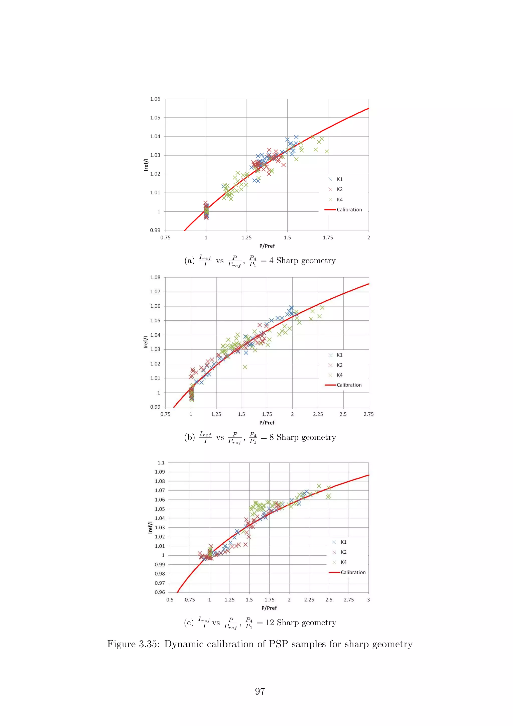
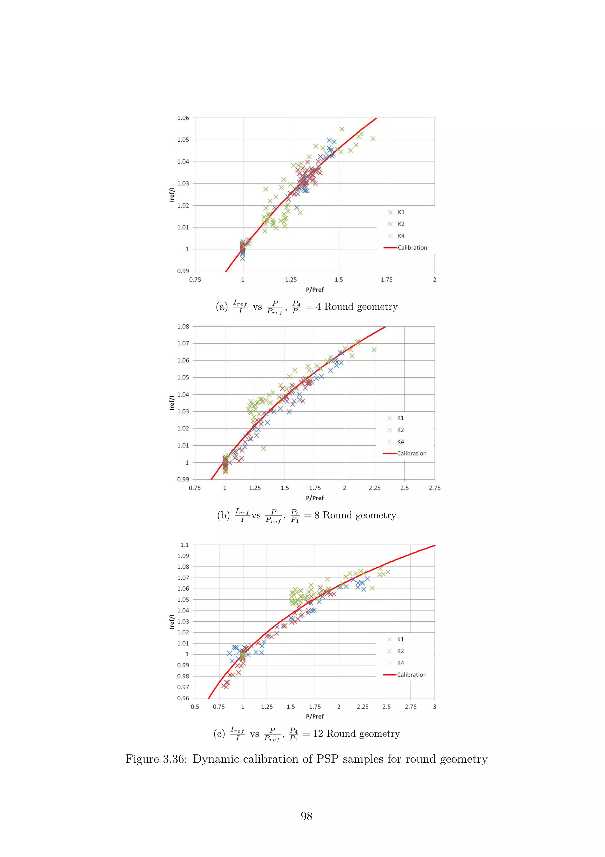
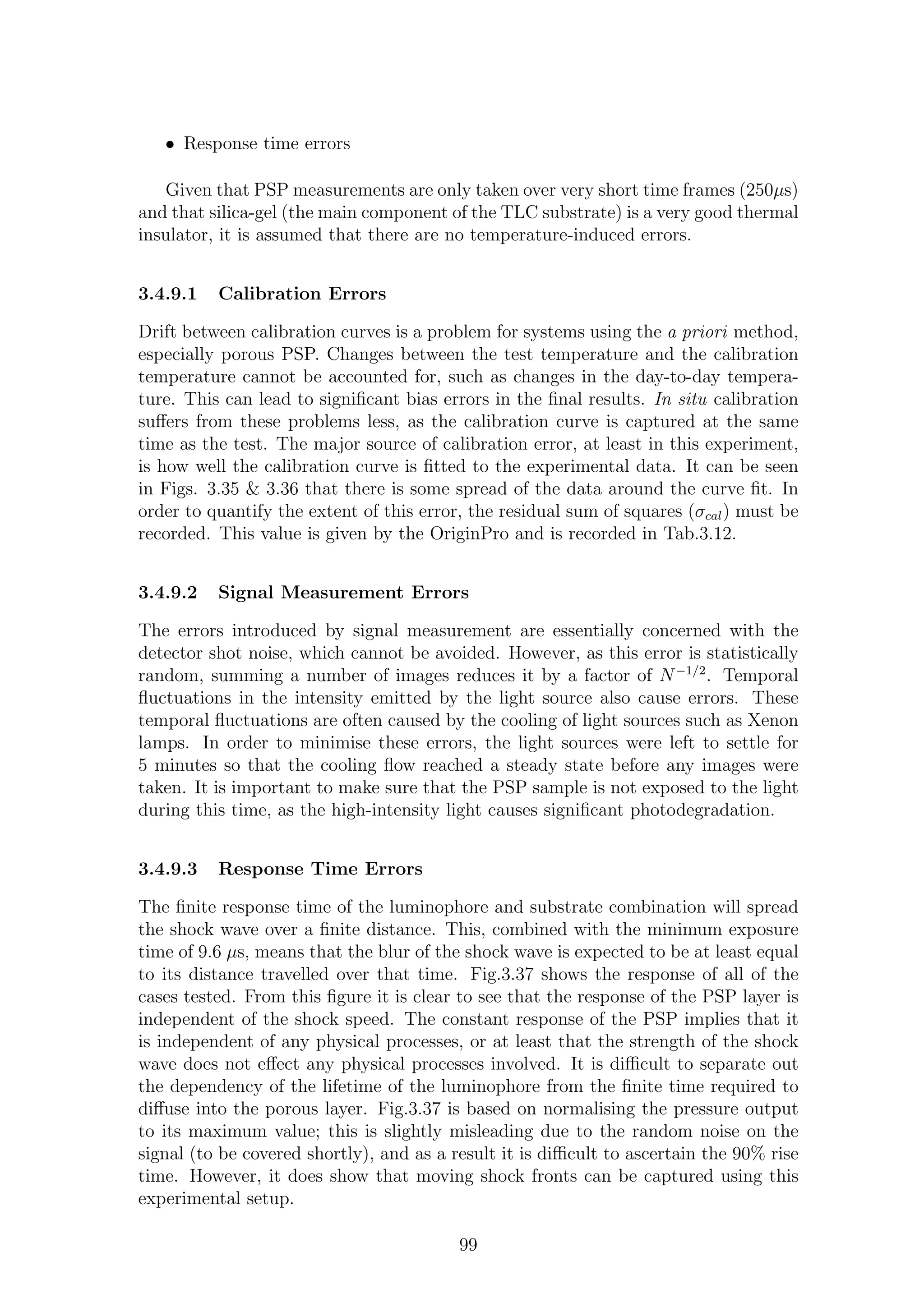
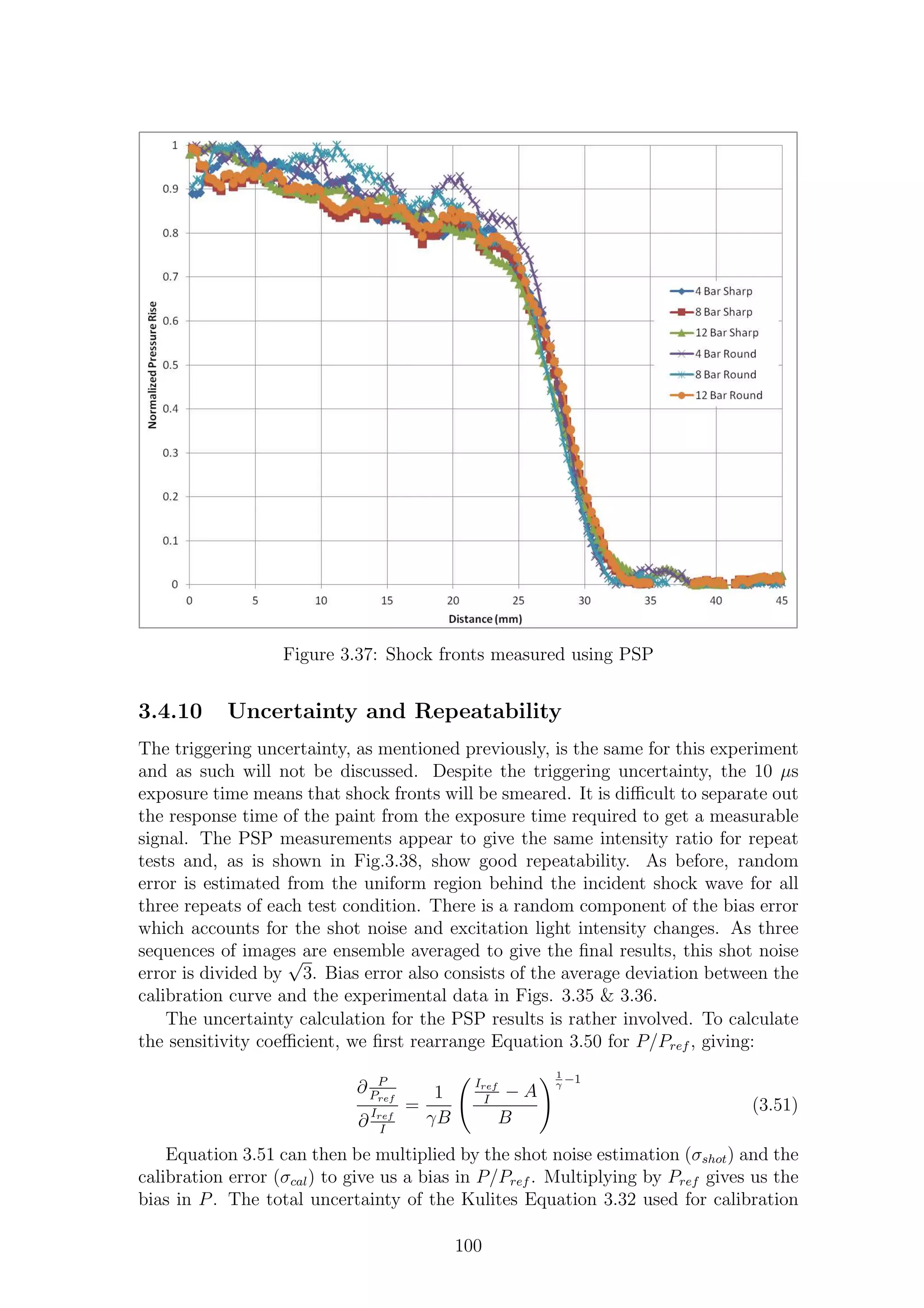
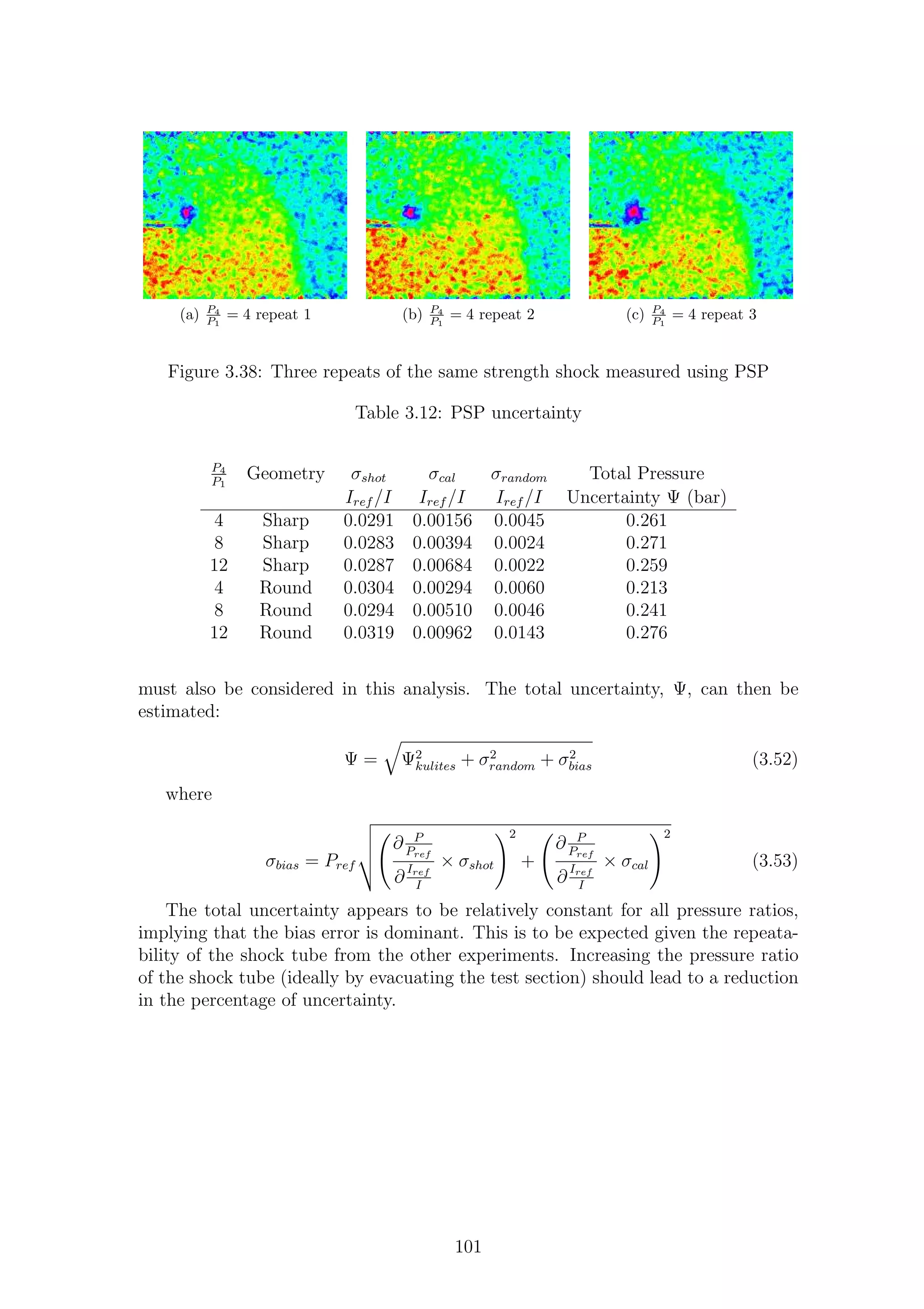

![Chapter 4
Apparatus
People like to imagine that because all our mechanical equipment moves
so much faster, that we are thinking faster, too - Christopher Morley
This chapter shows the experimental apparatus used in the tests and the numer-
ical procedure adopted.
4.1 Shock Tube
The shock tube is of square cross-section where the driver and driven sections are
the same cross-sectional size. The internal width and height of the shock tube is
24.8 mm and the external height and width is 30 mm, giving a wall thickness of 2.6
mm. The driver section is 0.7 m long and the driven section is 1.7 m long and is
open to the atmosphere. The plunger of the shock tube is pointed from the driver to
the driven section and has a spring-loaded sharp tip to rupture the diaphragm. The
diaphragm section comprises of two gaskets (one attached to the driver and one to
the driven) which are bolted together before pressurisation. The diaphragms used
are made of acetate and are of the minimum thickness required to stop premature
rupturing while pressurising the driver section. The minimum thickness is used so
that as little as possible of the energy of the shock wave is wasted, accelerating the
fragments of the diaphragm to the induced velocity, as discussed in Section 2.2.3.
The supports of the facility were, previously, rather flimsy and caused repeata-
bility issues [162]. New supports were manufactured in order to reduce vibrations
and enhance repeatability.
The calculation of x-t diagrams from the theory given in Section 2.2.1 allows
us to estimate the arrival time of the incident shock and run time of the shock
tube, i.e. the time before the contact surface reaches the test section or if the
reflected expansion head crosses the contact surface. This calculation is based on
the experimental Mach number from Section 3.1.7. Fig.4.1 shows the x-t diagrams
based on Mie as calculated by a Matlab code written by the author. The test times
and shock arrival times are given in Tab.4.1.
4.1.1 Test Section
The test section is made of perspex, with interchangeable side walls so that different
experiments can be performed. Using the standard perspex walls, schlieren and
103](https://image.slidesharecdn.com/4a6f74b5-6bbb-4ffd-b3f5-7486cdb057cd-150303082443-conversion-gate01/75/Mark-Quinn-Thesis-134-2048.jpg)
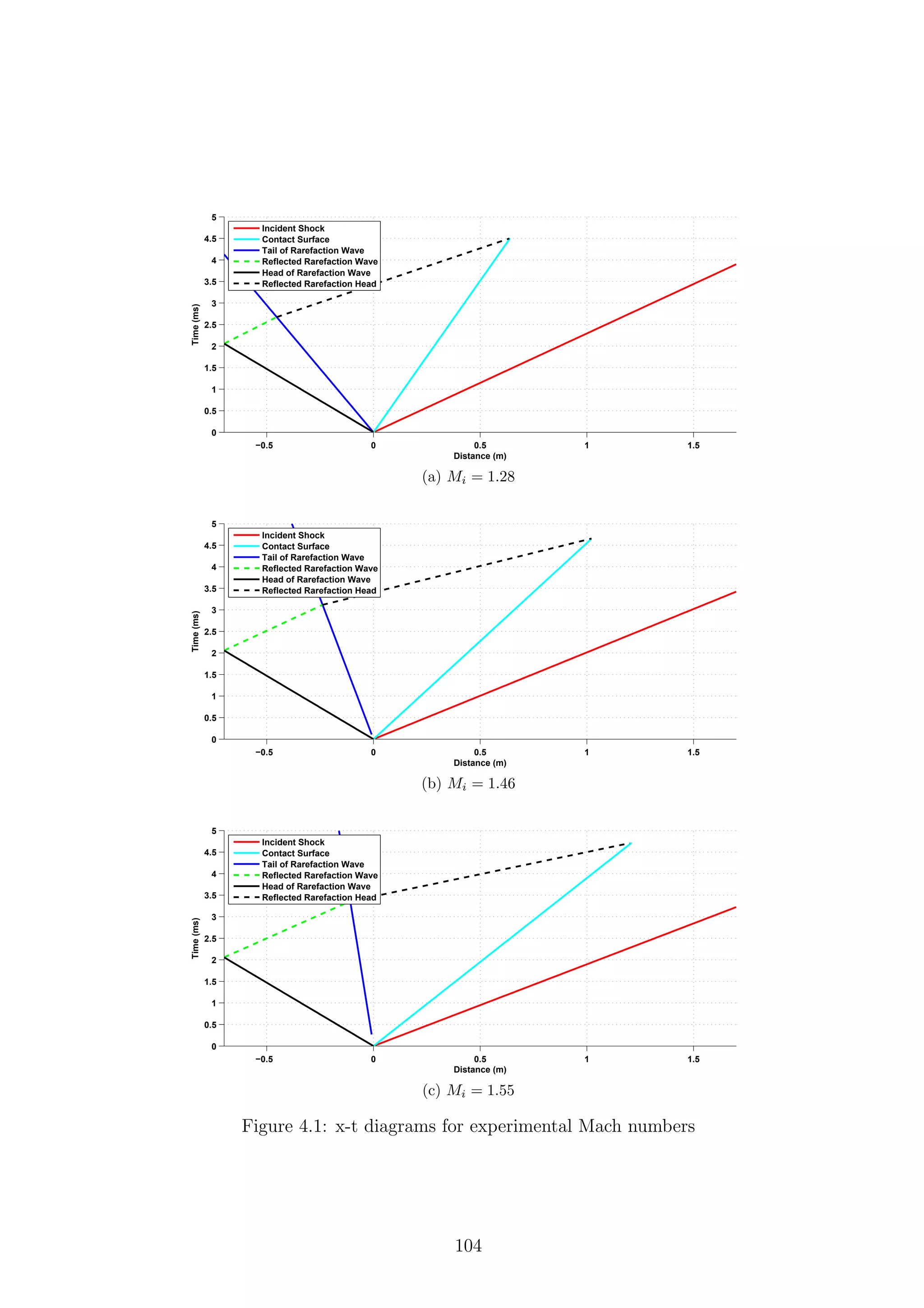
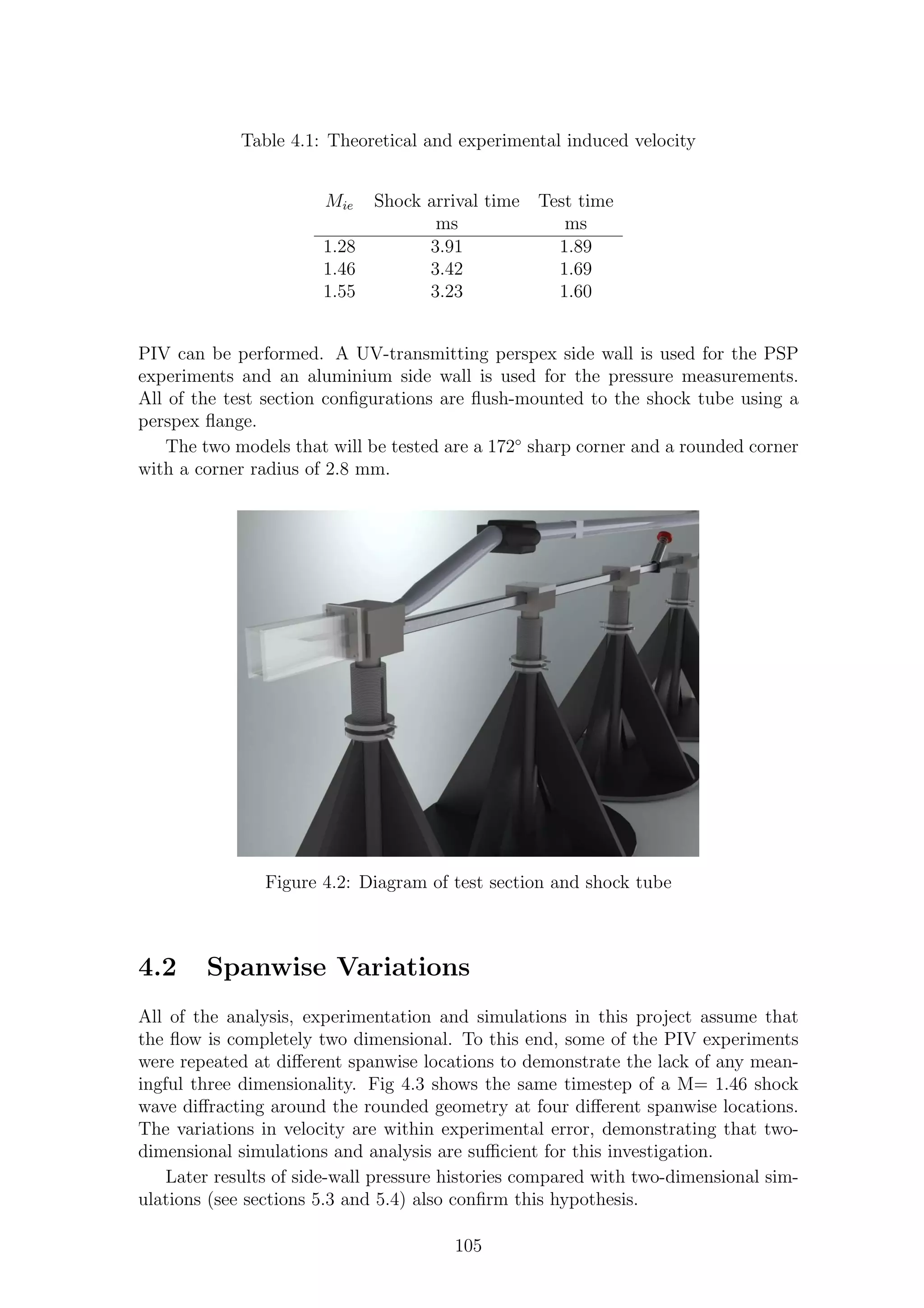
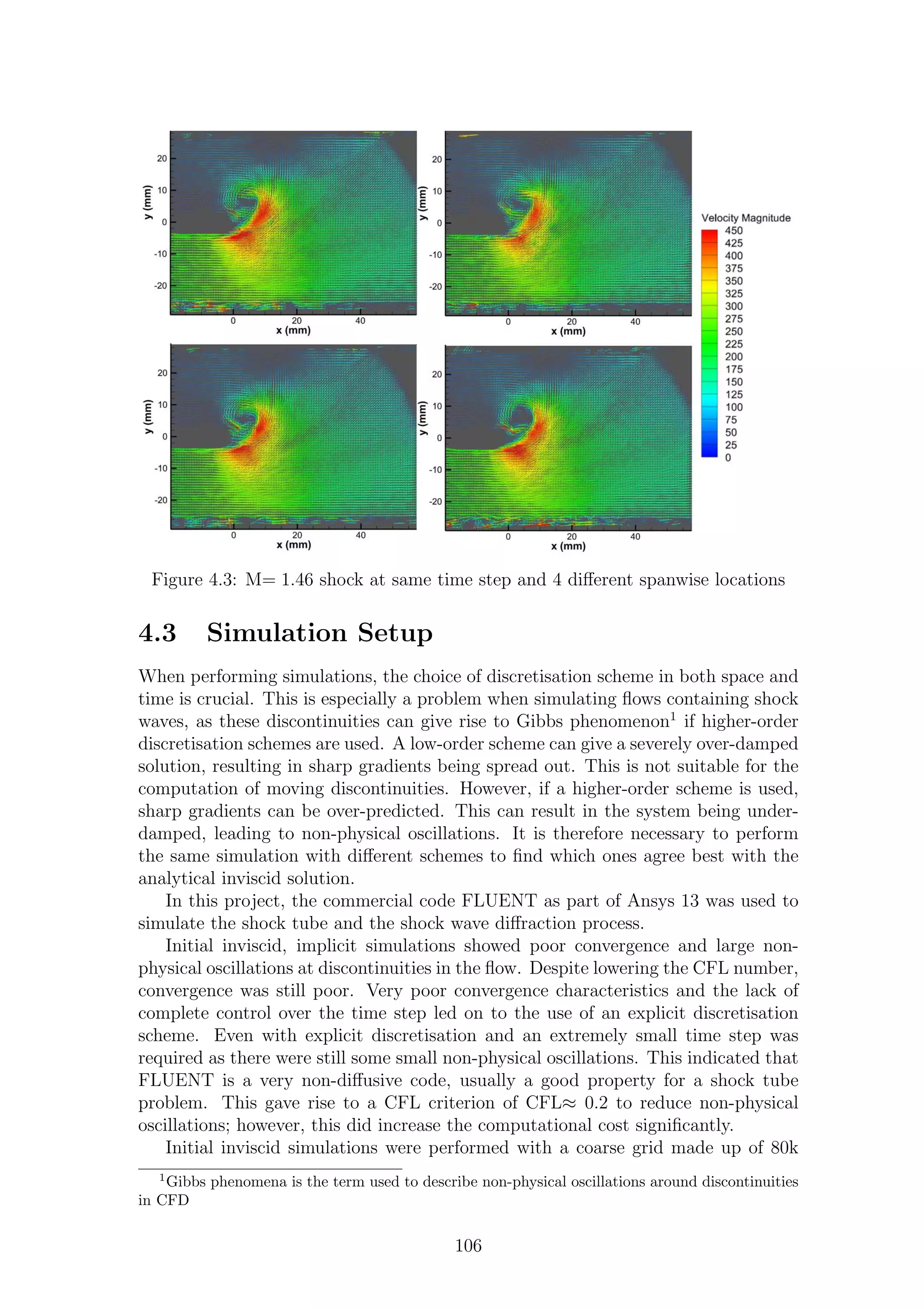
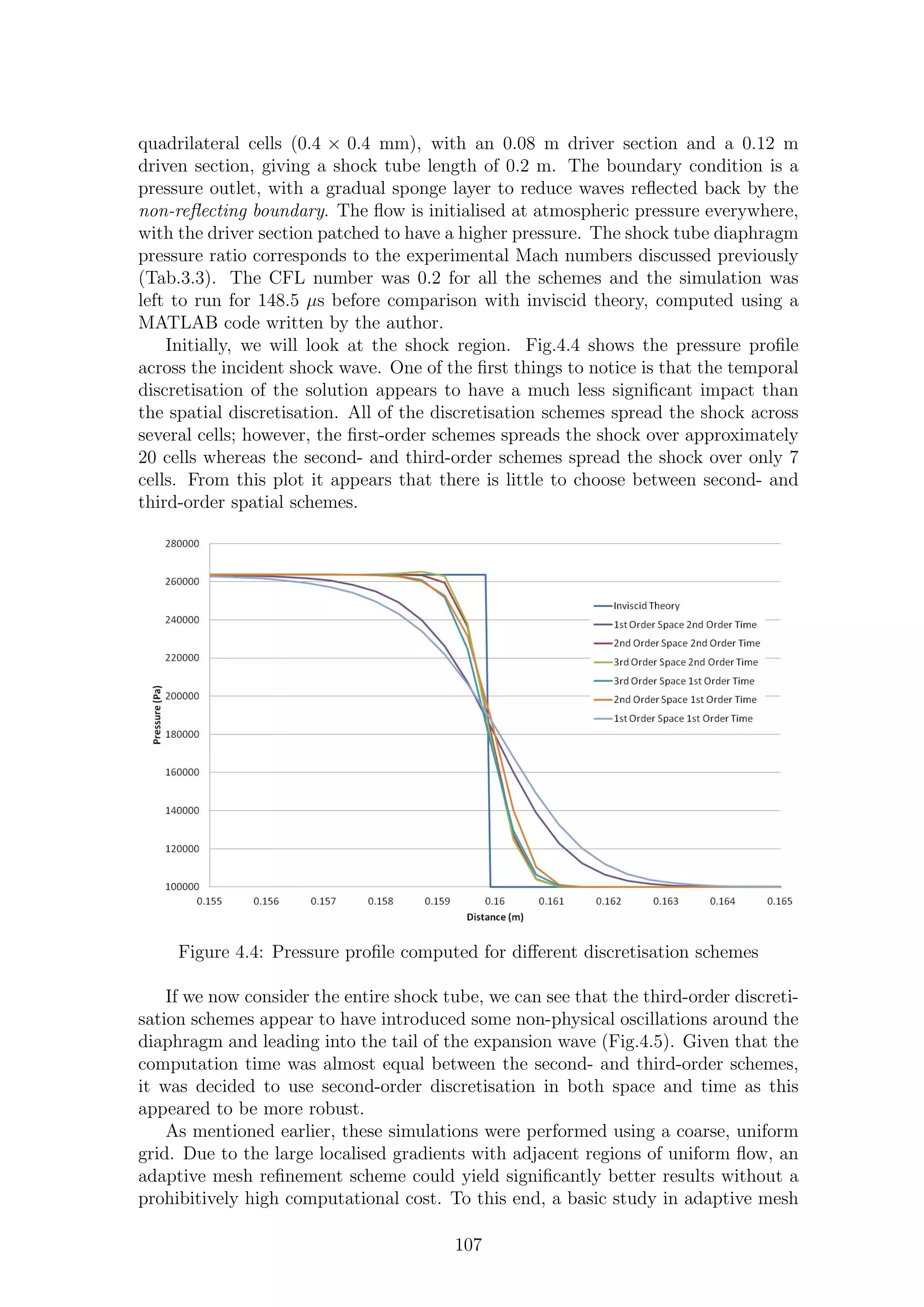
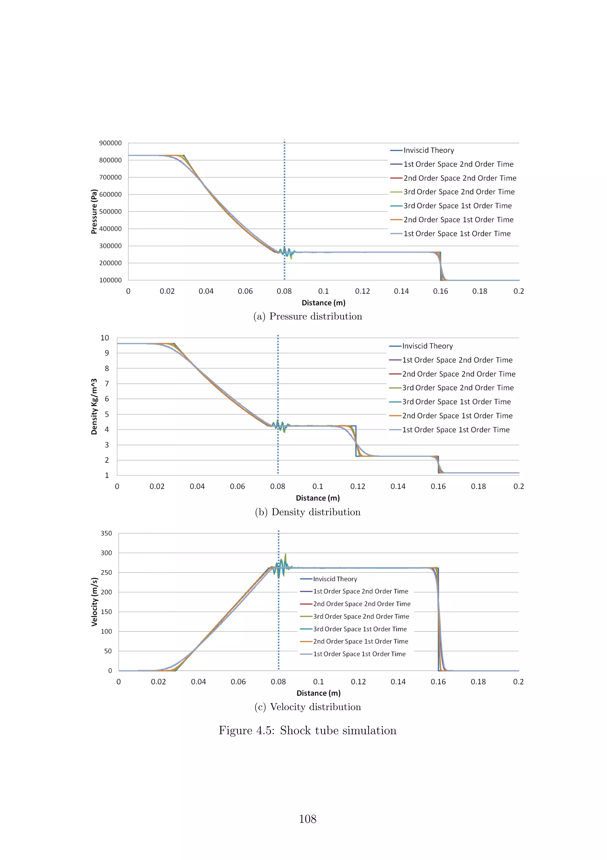
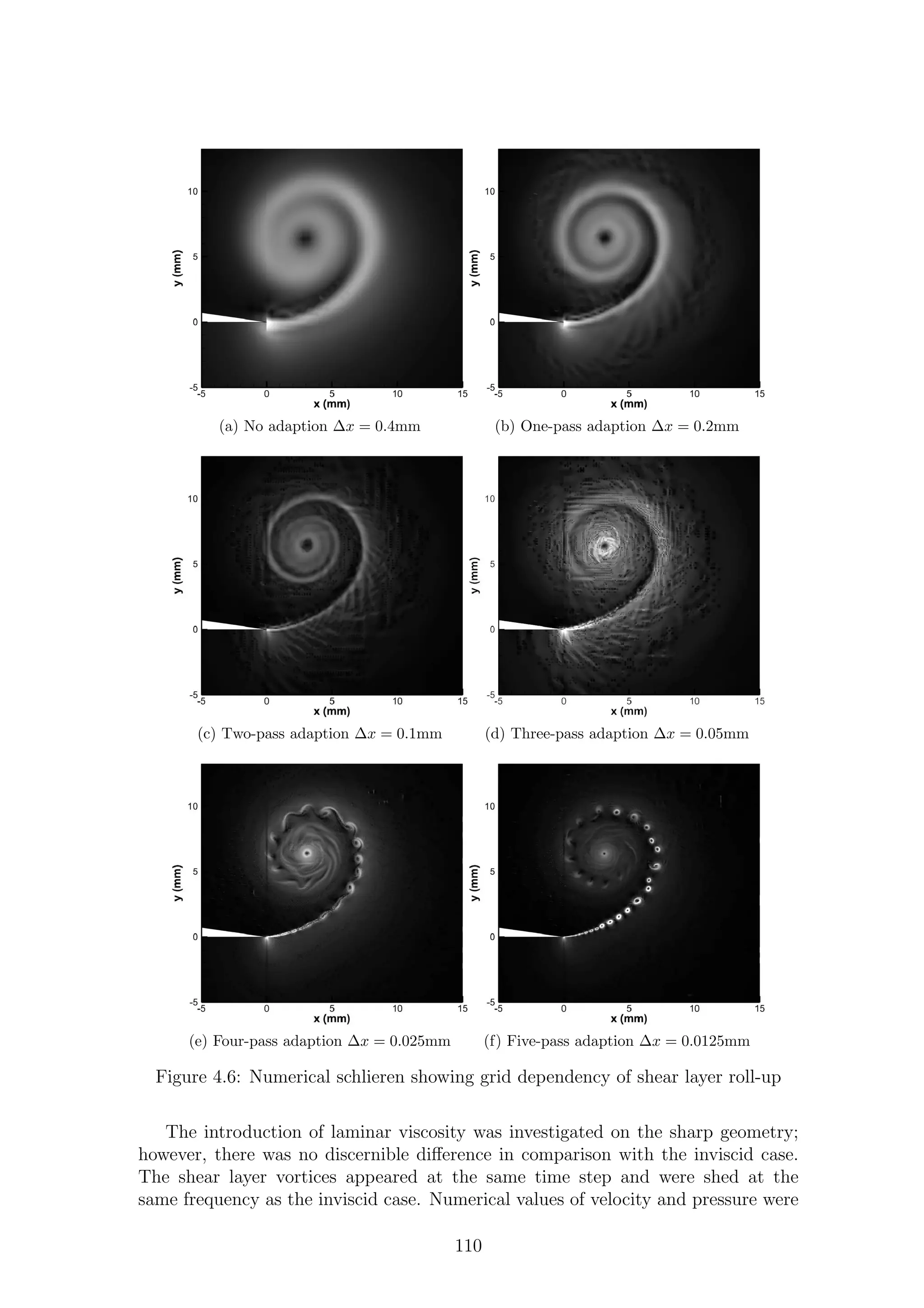
![marginally different, but the dominant shock structure was the same.
4.3.2 Round Geometry Grid Dependency
Based on the successes of the previous simulations, it was decided to attempt a
similar simulation of the round geometry. Fig.4.7 shows the same time step using
an inviscid solver at two different grid refinements. The initial coarse grid (Fig.4.7a)
shows a shock wave at approximately 85◦
around the corner with no flow separation.
The shocks are not very well captured, similarly to the coarse results seen previously.
Refining the grid had the effect of resolving the shock waves; however, there was
still no sign of flow separation. This is contrary to the experimental results (to be
shown later) and previously published literature ([42],[44],[46]). This shows that an
inviscid simulation is not capable of resolving all of the relevant flow features.
(a) Inviscid simulation, coarse grid (b) Inviscid simulation, Four-pass adaption
Figure 4.7: Numerical schlieren of inviscid simulation around round geometry
The associated length scale (radius of the corner) means that separation is not
induced by a sharp point and the separation of the flow is a viscous effect. The
introduction of laminar viscosity should be sufficient to model the separation of the
flow around the corner [199]. Simulations performed using laminar viscosity with
different levels of grid refinement are shown in Fig.4.9.
A new mesh was generated with the boundary layer resolved. The minimum cell
size in the boundary layer was 13 µm and the boundary layer was wrapped around
the corner as shown in Fig.4.8 as well as along the top and bottom walls of the
shock tube and the test section. Unfortunately, due to the round geometry, it was
necessary to include a portion of the mesh as tetrahedral rather than quadrilateral
cells. These cells are, at most, half the size of the quadrilateral cells in the rest of the
grid, and as such the minimum grid size in this region is lower than the ∆x = 0.025
mm seen in the previous four-pass adaption cases. The computational cost of these
simulations is significantly higher than the inviscid simulations, as the addition of
viscosity led to localised convergence issues in some cells at the shock foot.
Simulations performed using turbulence models tended to incorrectly predict the
boundary layer separation. A Reynolds stress model was also tried; however, the
111](https://image.slidesharecdn.com/4a6f74b5-6bbb-4ffd-b3f5-7486cdb057cd-150303082443-conversion-gate01/75/Mark-Quinn-Thesis-142-2048.jpg)
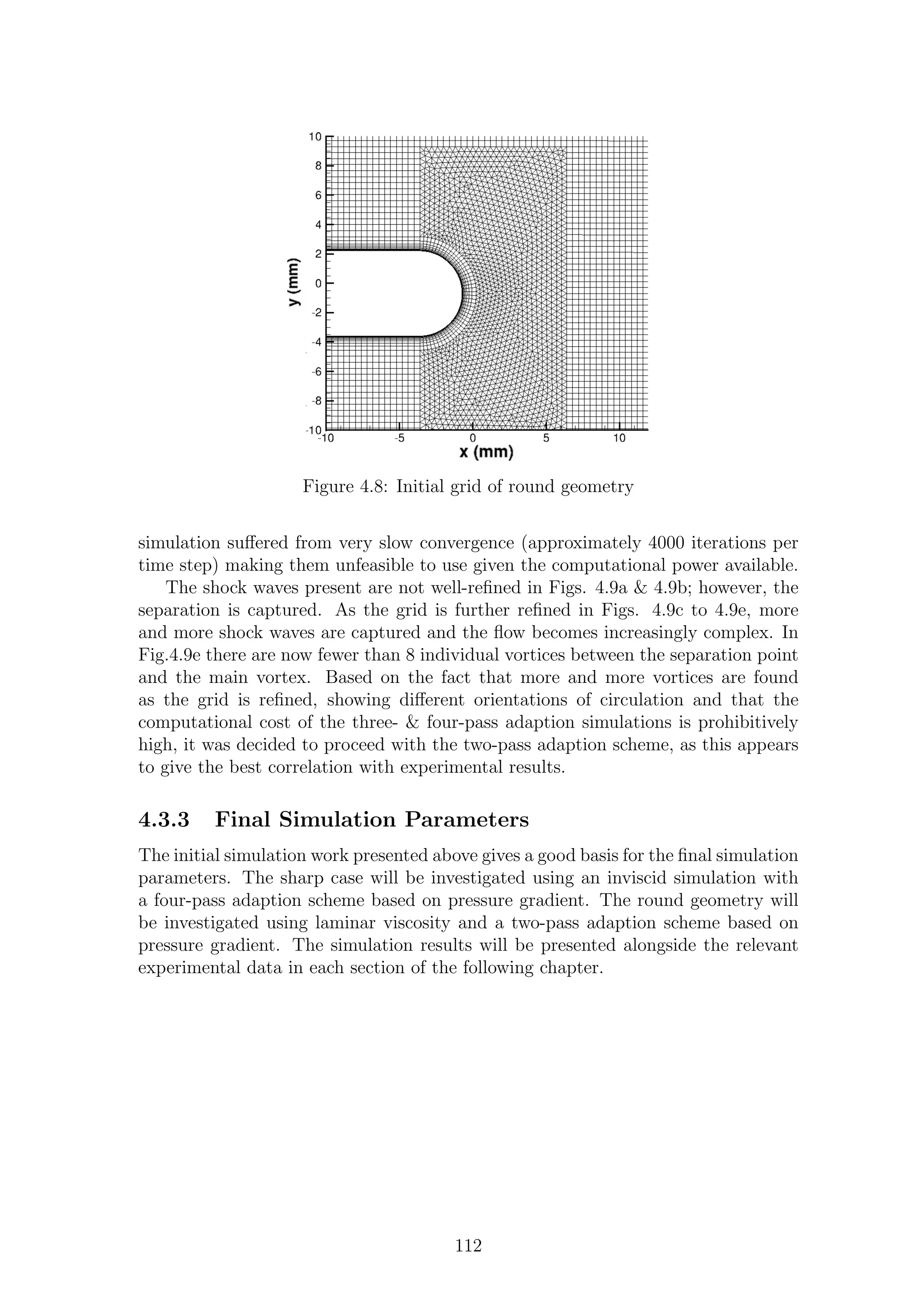
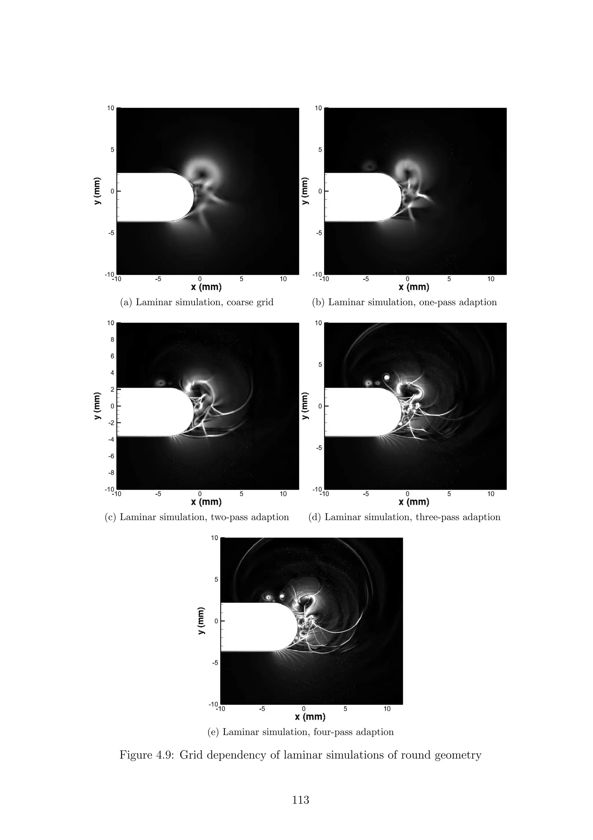

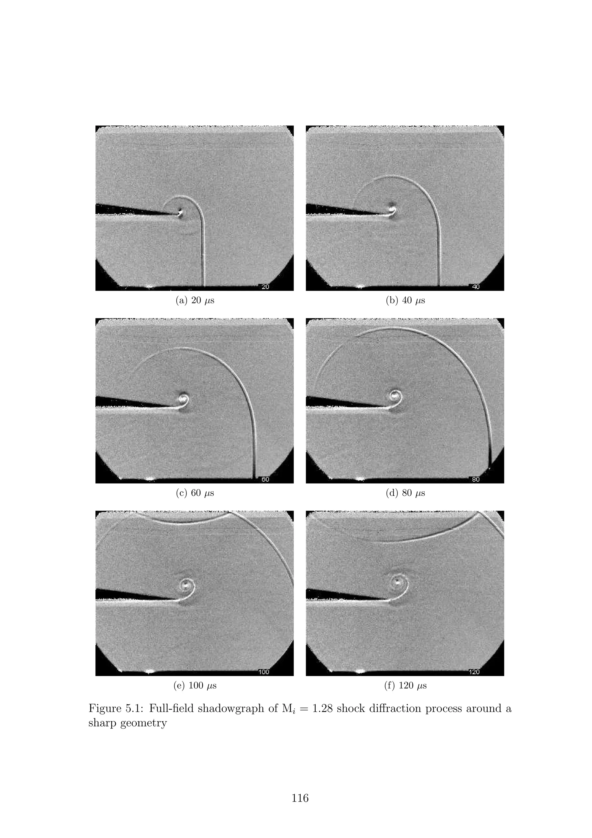
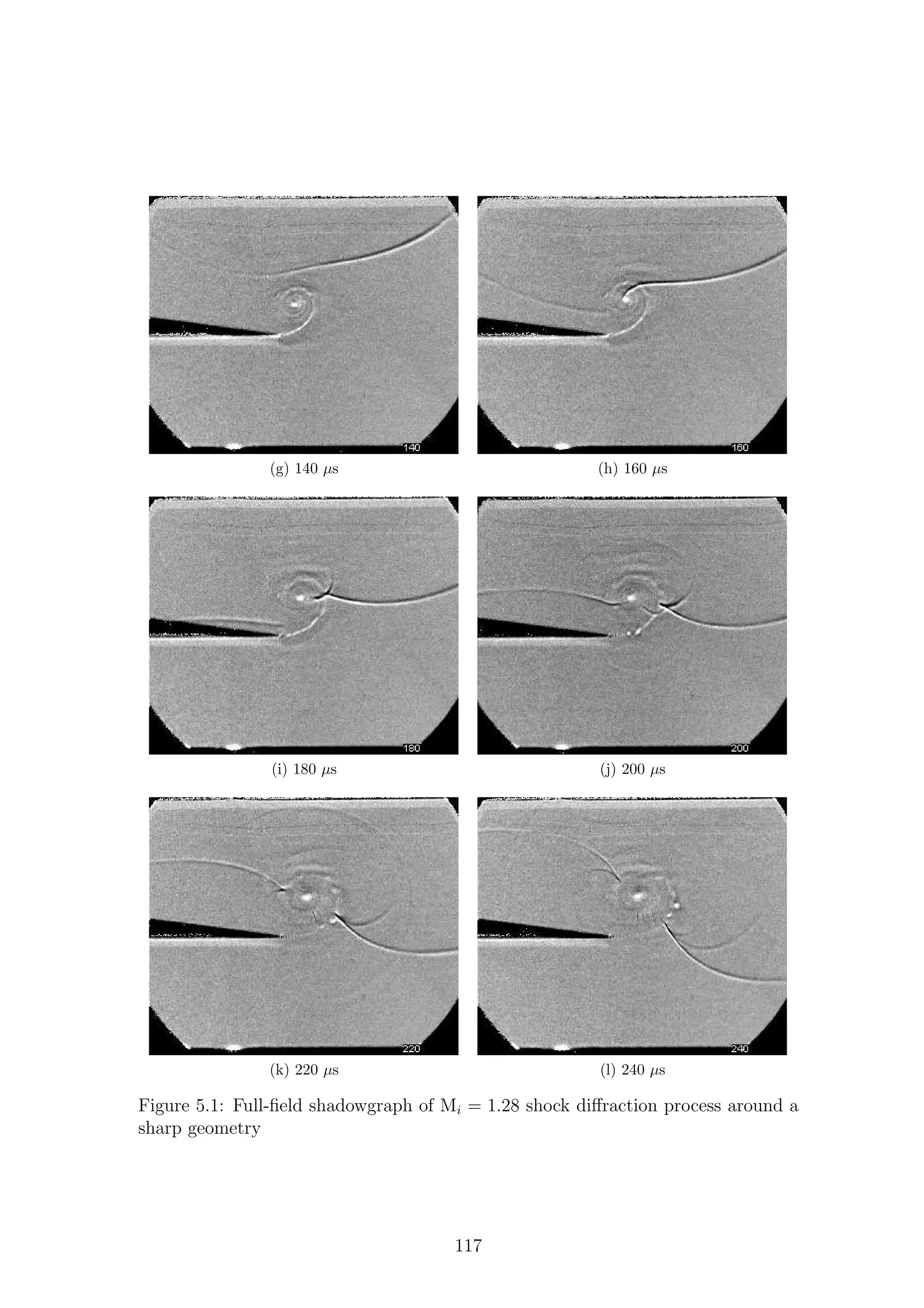
![the shock wave while the flow on the left does not. By Fig.5.1h it is clear that the
returning shock wave is beginning to be split by the main vortex; the right-hand
side forms a Mach reflection, with the Mach stem inside the shear layer appearing to
be connected to the centre of the vortex. As the waves propagate further, the Mach
stem appears to travel faster than the wave structure outside of the shear layer and
begins to disperse into weaker waves. Meanwhile, the accelerated returning wave
on the left of the vortex has impinged on the splitter plate. Figs.5.1i to 5.1l do not
show much distortion to the shape of the shear layer; however, two strong vortices
are formed, as was seen by Skews [71].
The full-field schlieren images in Fig.5.2 show some of the flow features more
clearly than the shadowgraph images in Fig.5.1. The contact surface between the
gas affected by the planar shock and the curved, diffracted shock is visible and the
reflected expansion wave is propagating upstream. There is very limited information
available in Figs. 5.2a to 5.2f about the vortex and the shear layer as the density
changes in this region are strong enough to overrange the schlieren system. After
120 µs the vortex has grown in size to a level where the local gradients are no longer
strong enough to overrange the system. From Fig.5.2g onwards, there appear to be
several bumps serially arranged around the shear layer. These bumps are, as we will
see shortly, the Kelvin-Helmholtz instability on the shear layer. In Fig.5.2j, the two
strong vortices formed from the impact of the returning shock on the shear layer are
clearly seen. There is little more to say about the shock-vortex interaction process
further than what was shown in the previous figure; however, there is a region of
flow which appears much darker in Figs.5.2j & 5.2k, indicating a strong interaction.
In the close-up shadowgraph images, as expected, the sensitivity of the system
is higher, and as such more flow features are visible. Unlike in Fig.5.1, the reflected
expansion wave can be seen in Figs.5.3a & 5.3b before it has passed out of view.
The contact surface is also visible throughout the sequence and can be seen to be
pulled into the centre of the vortex. Even as early as 80 µs we can begin to see
changes in intensity along the shear layer, indicating the presence of disturbances.
As the vortex grows, these disturbances become accordingly larger, allowing us to
see individual vortices present on the shear layer. These individual vortices grow
and are clearest at approximately 90◦
around the vortex (starting from the splitter
tip)1
. After this point the vortices begin to dissipate and become more diffuse until
they are indistinguishable by approximately 300◦
.
Following the impact of the returning shock on the splitter plate (Fig.5.3i on-
wards), the shear layer again shows two large disturbances, followed by a region
showing a repetitive alternating light and dark pattern. It is not possible to dis-
cern from these images what this exact structure is. In Fig.5.3j the returning shock
wave on the right of the vortex is split into a complex structure involving a Mach
reflection in close proximity to a regular reflection. This only appears outside the
shear layer, which seems to act as a barrier. The final image, Fig.5.3l, shows a
series of diverging waves that emanate from the shear layer and are connected to
the returning shock wave. This is a series of diverging acoustic waves created by the
interaction of the shock with the individual K-H vortices on the shear layer, similar
to that investigated by Chang & Chang [72].
1
All angles noted in descriptions of flow features around the vortex start from 6 o’clock and
progress anticlockwise
118](https://image.slidesharecdn.com/4a6f74b5-6bbb-4ffd-b3f5-7486cdb057cd-150303082443-conversion-gate01/75/Mark-Quinn-Thesis-149-2048.jpg)
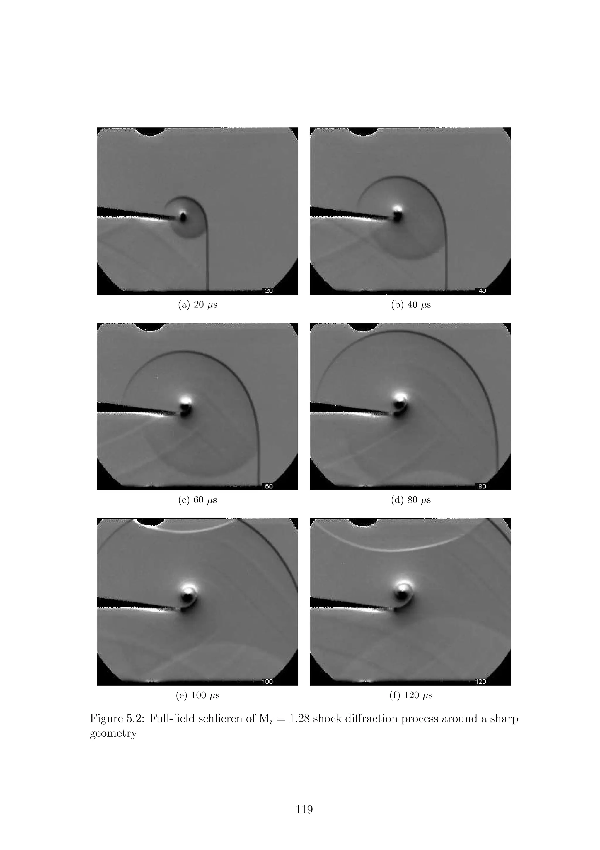
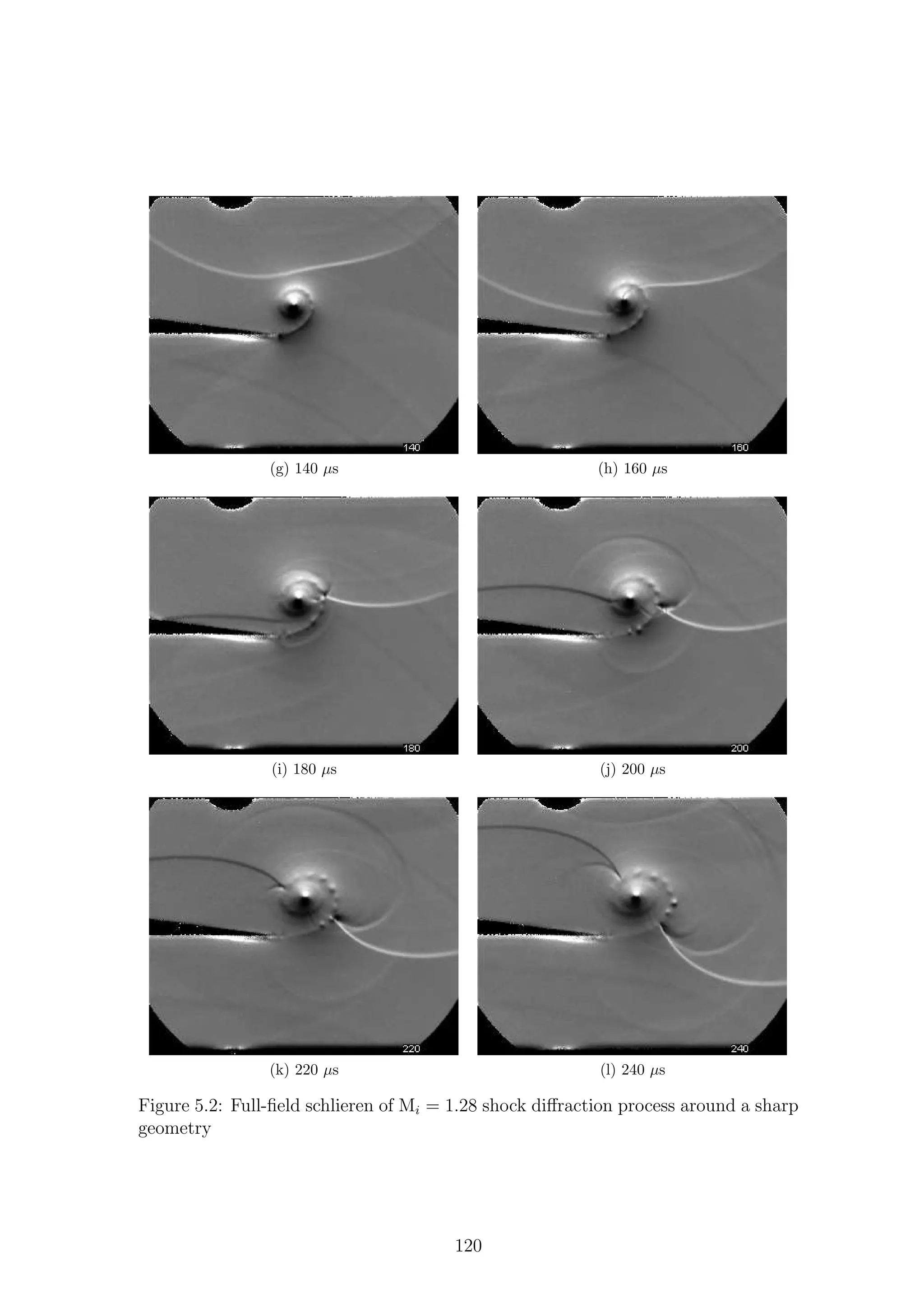
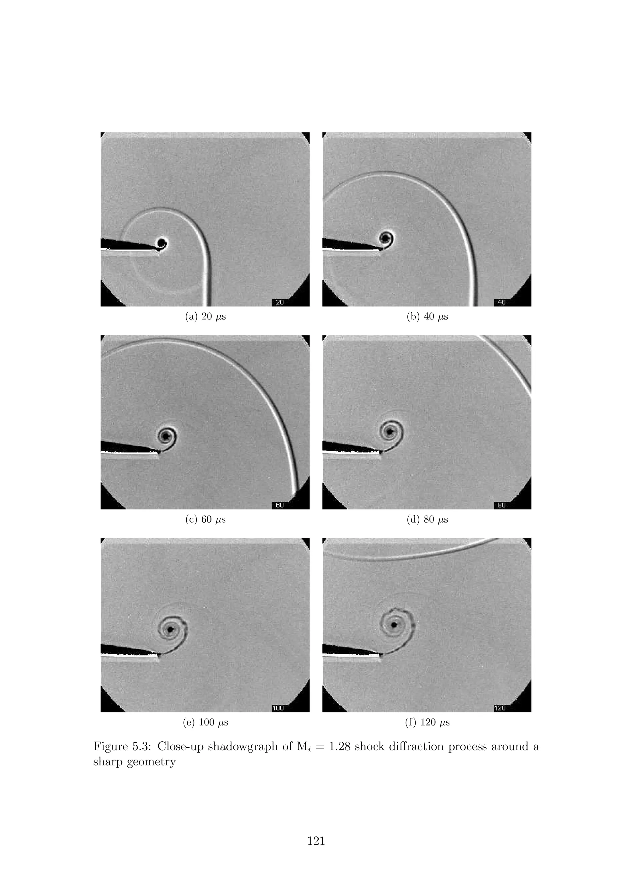
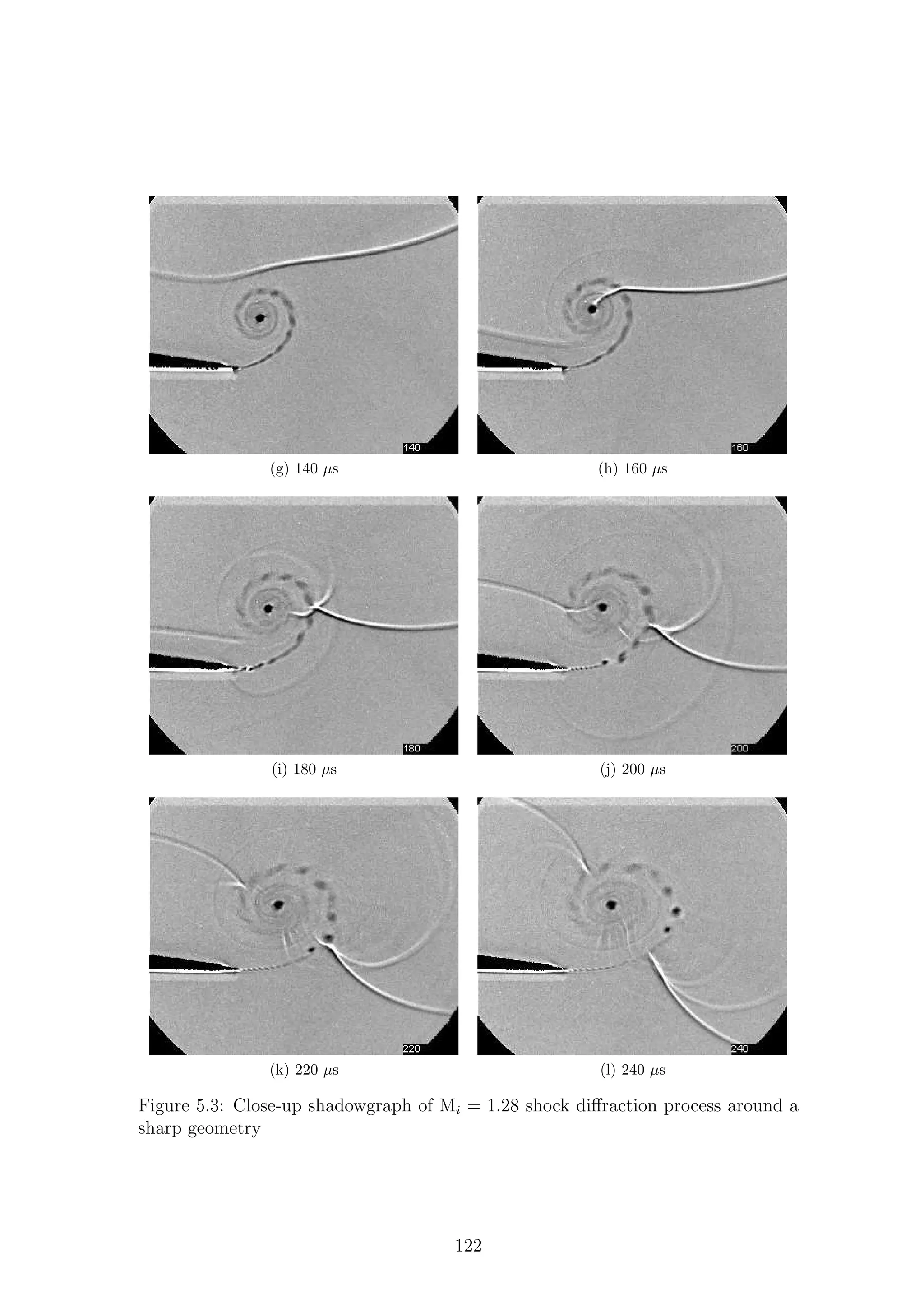
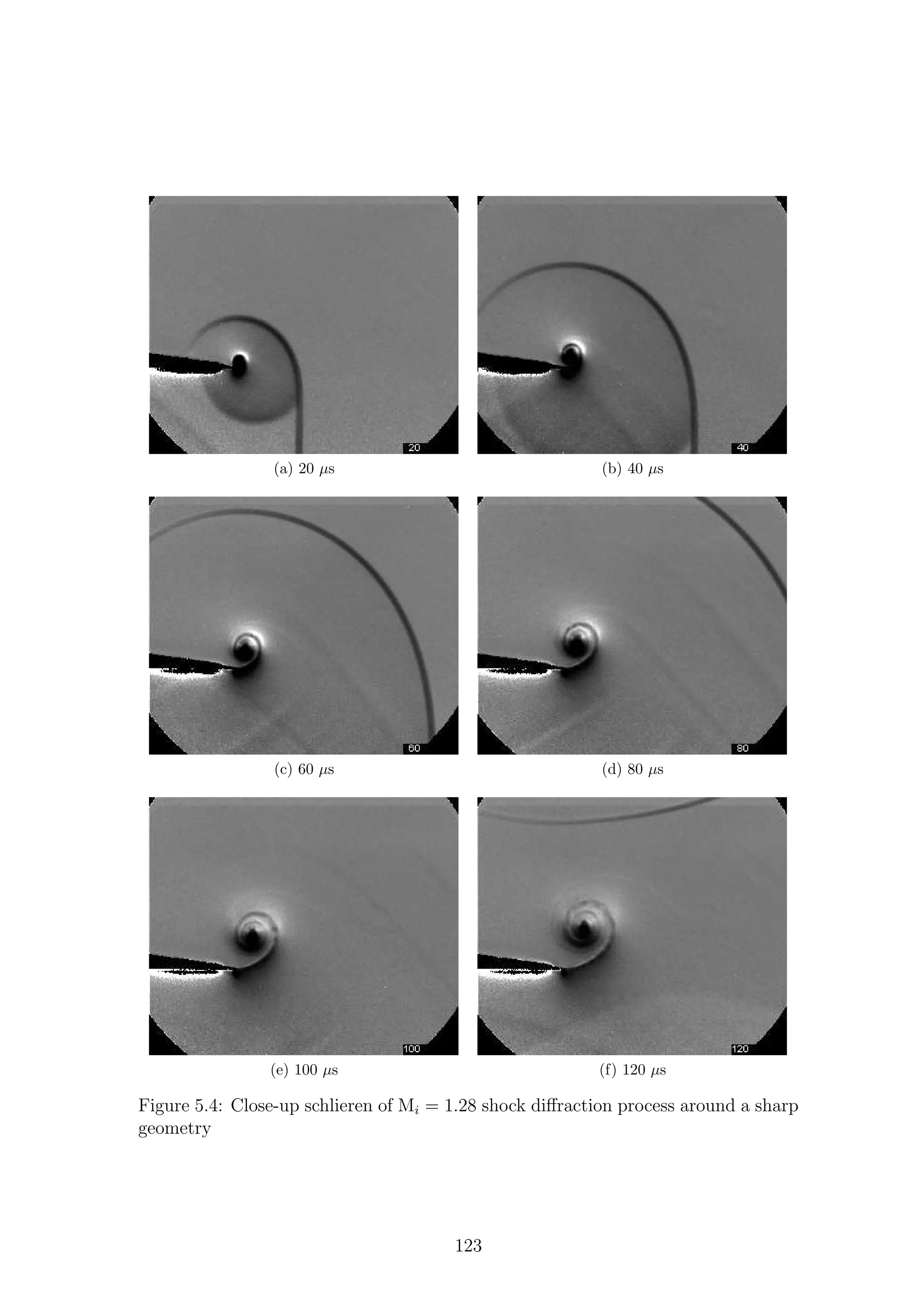
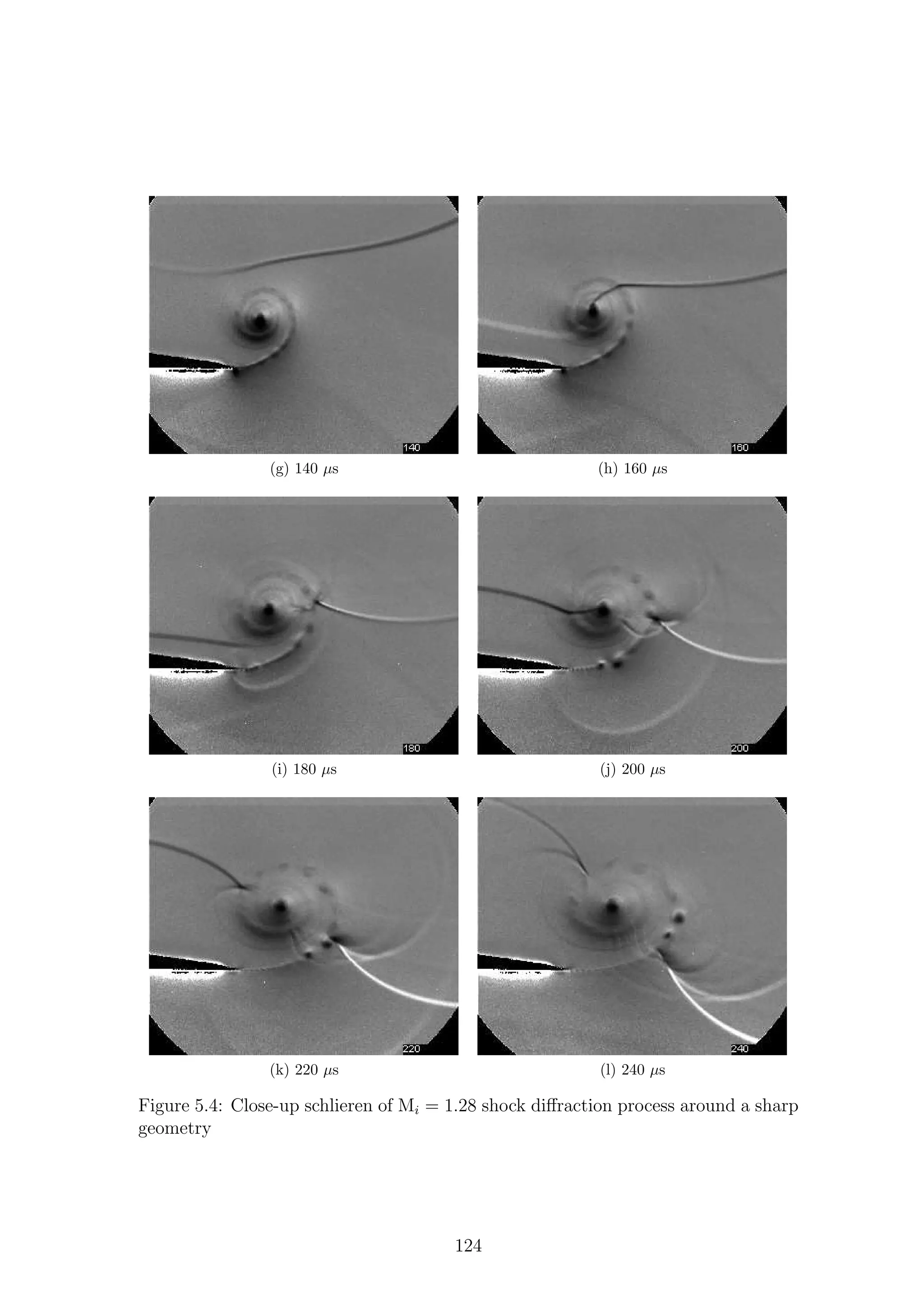
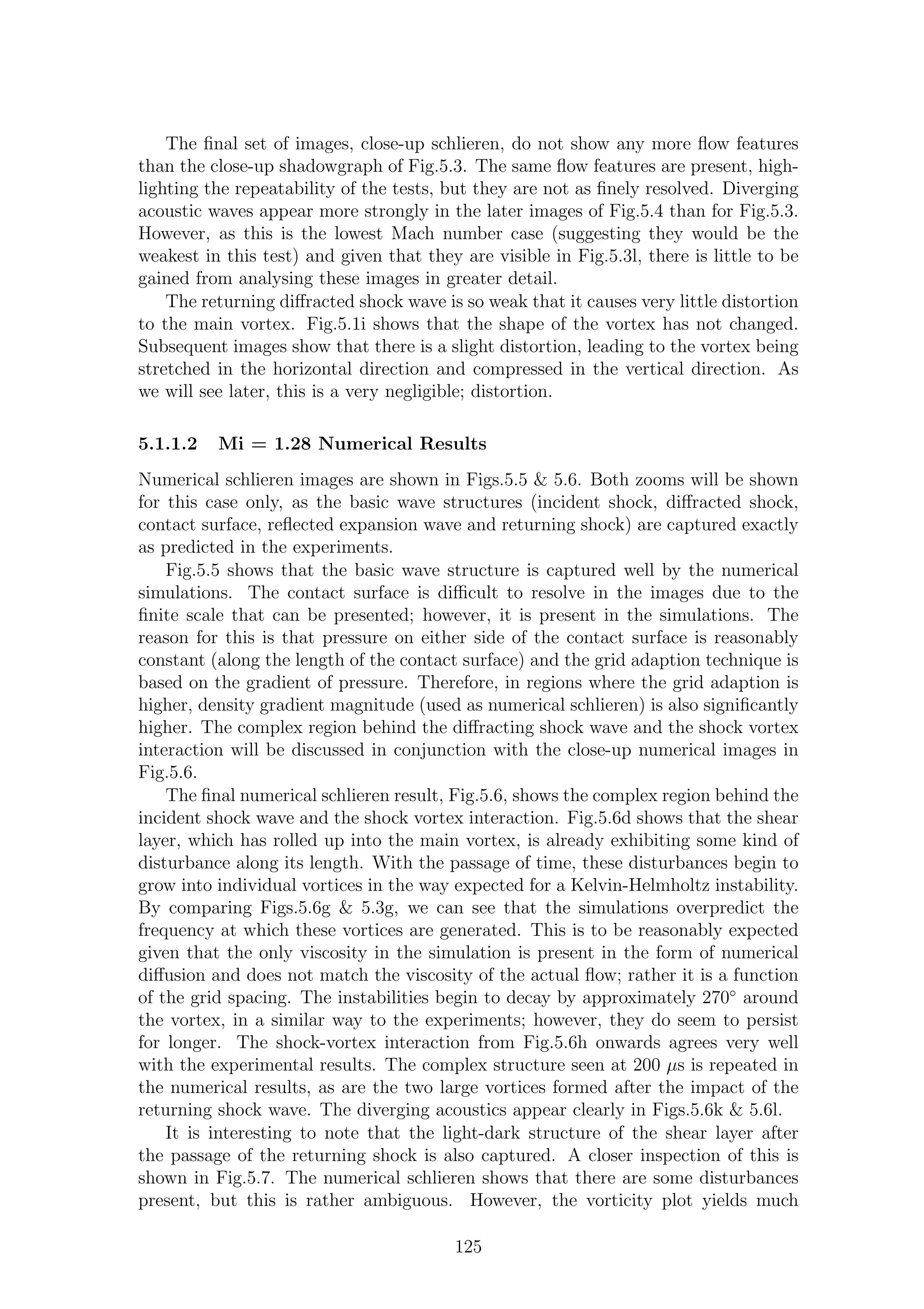
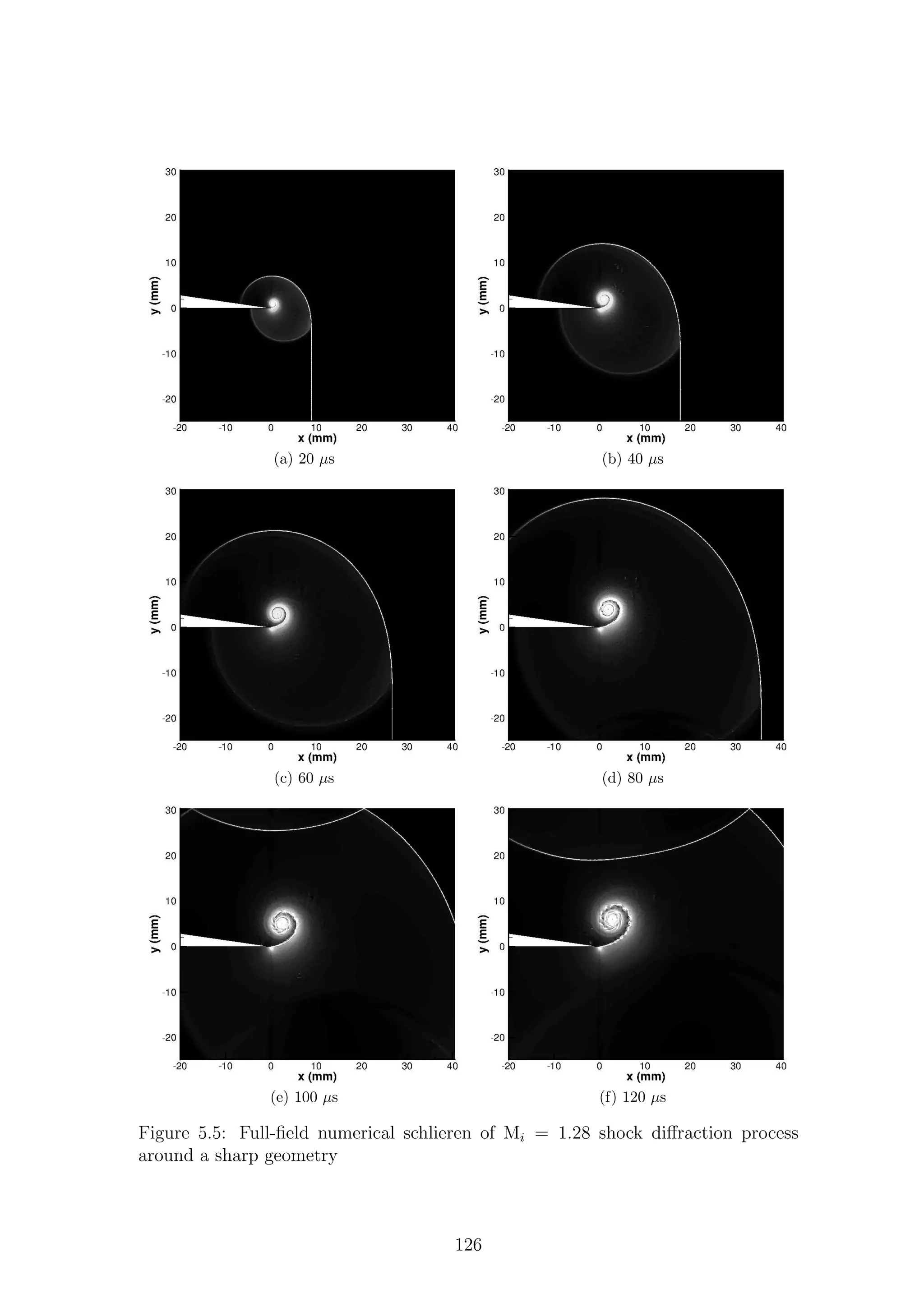
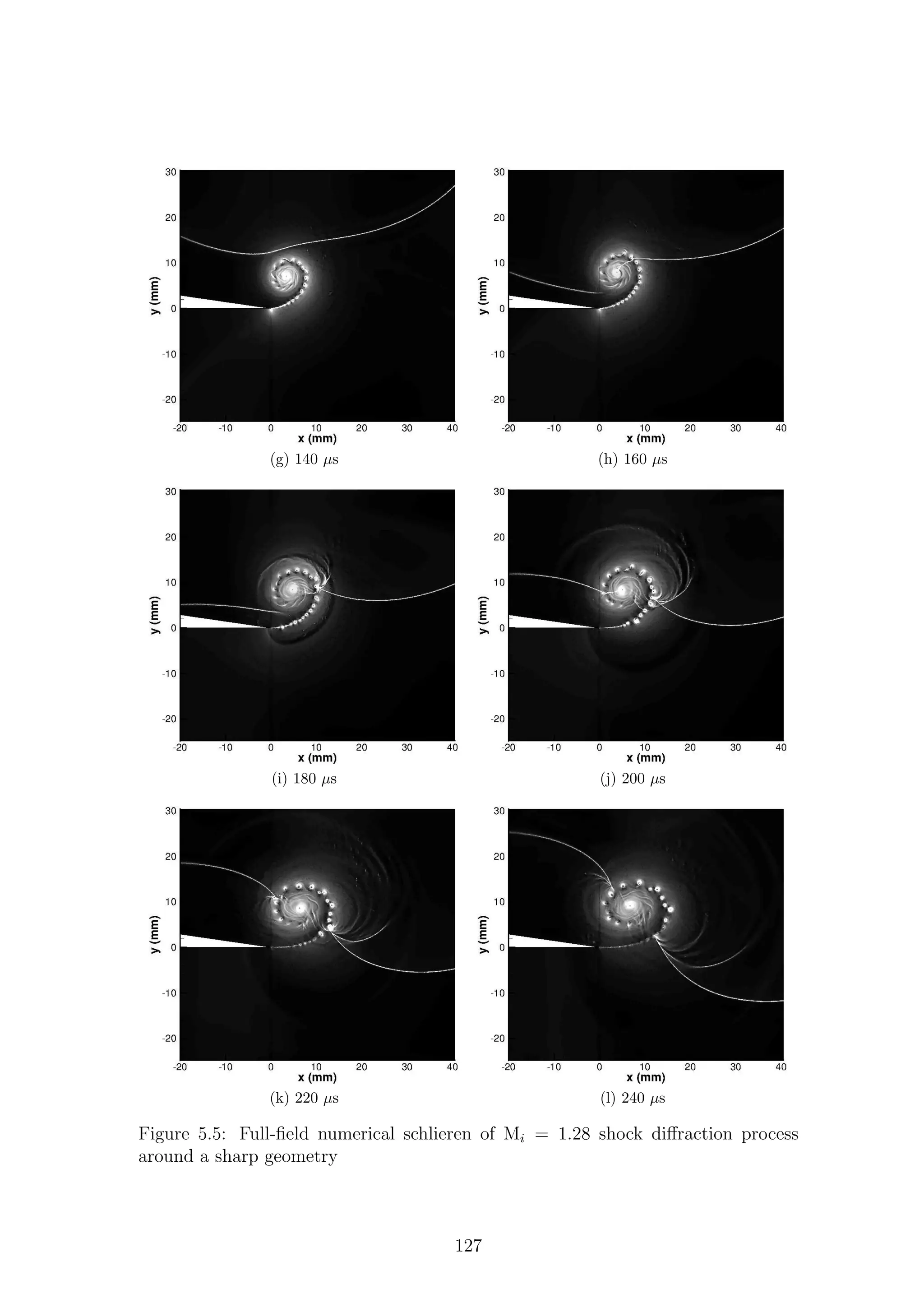
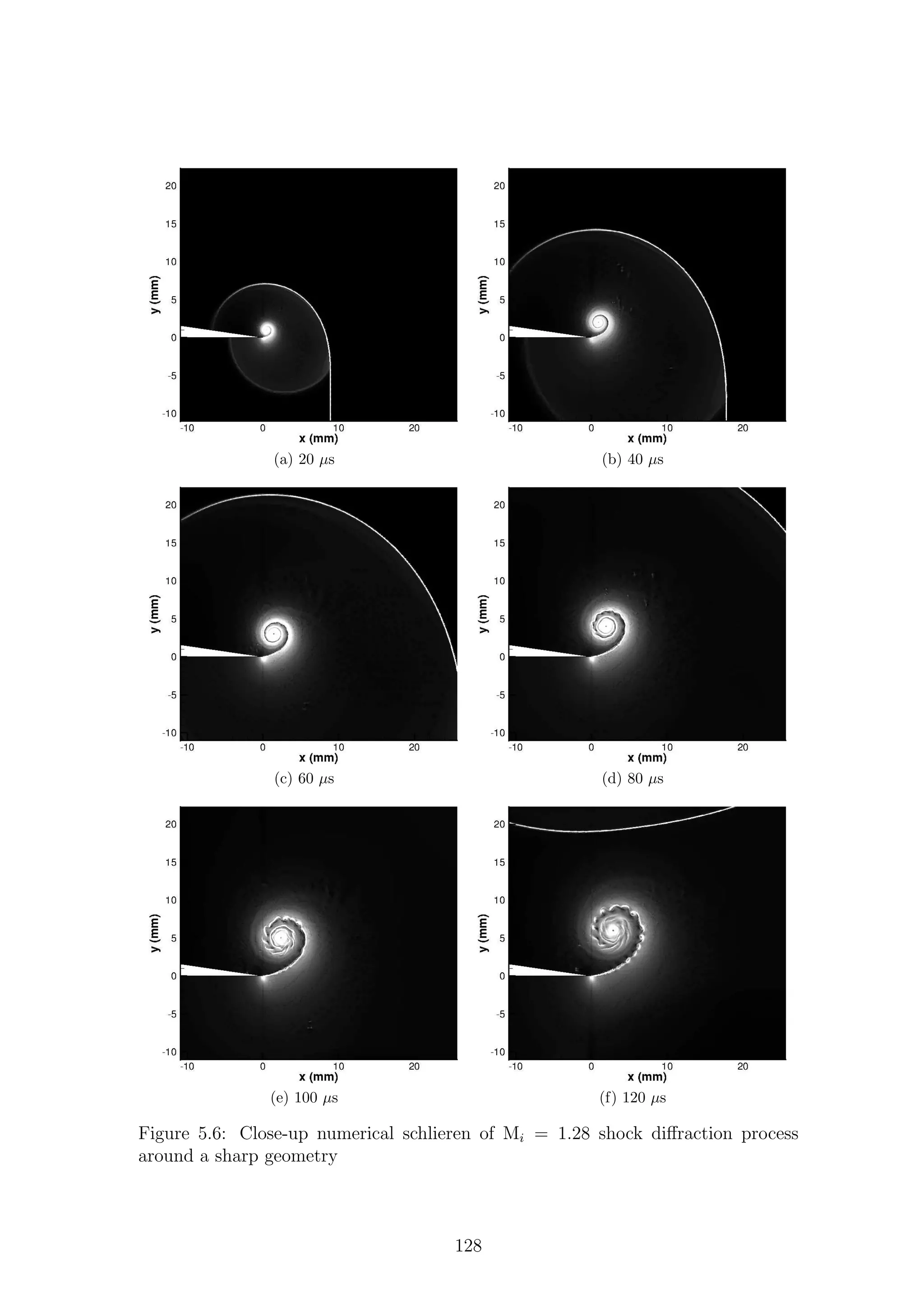
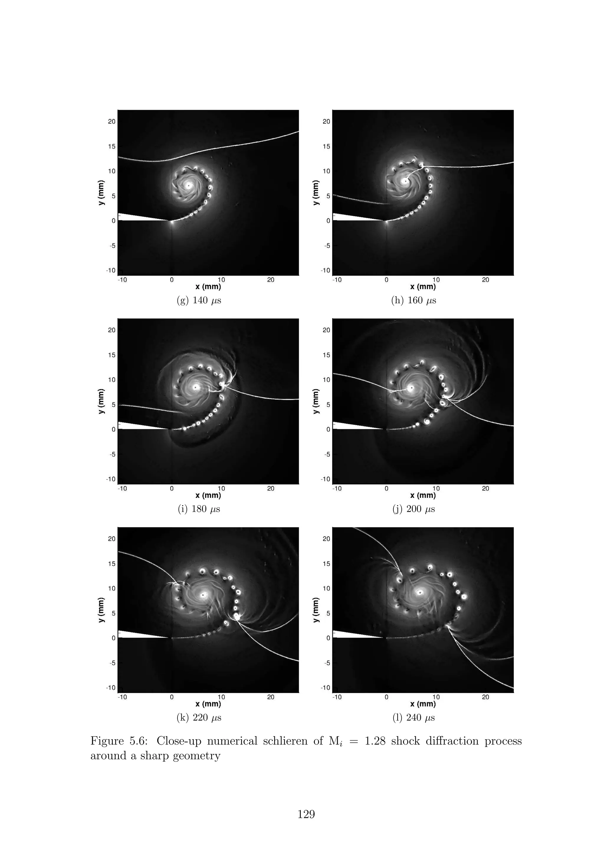
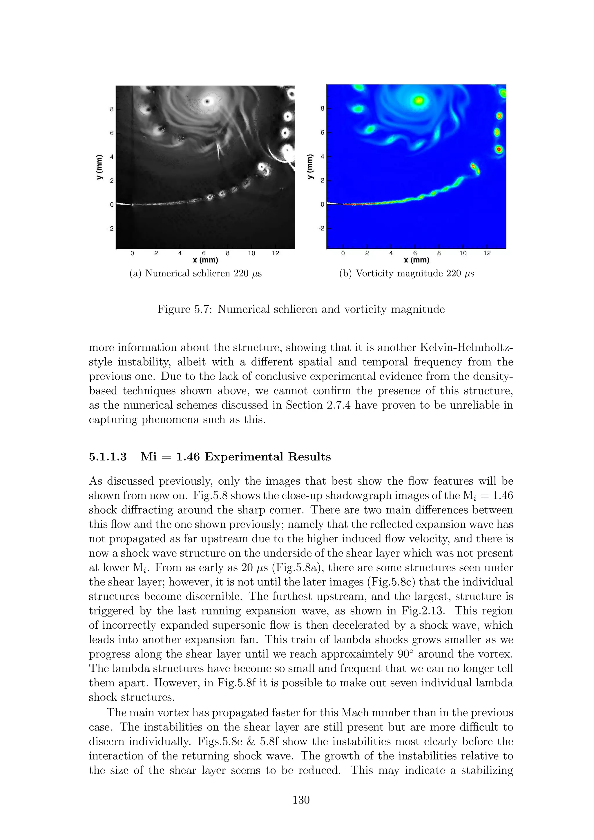
![effect as the velocity ratio across the shear layer increases. The diffracted shock
wave slows down the motion of the shear layer instabilities, making them more
visible in Figs.5.8i to 5.8l. This could indicate that, the motion and small scale of
these vortices means that they are blurred together in the experimental images.
The diffracted shock wave does not return from the top wall of the test section
any more quickly in this case than in the previous one, indicating that it is travel-
ling at almost sonic speeds. However, the higher induced velocity (especially in the
expansion region) and the stronger vortex generated means that the shock vortex
interaction is much stronger in this case. Fig.5.8h shows the early signs of a trans-
mitted wave that was not present at this time in the previous case. On the right
hand side of the vortex, as before, the returning shock wave forms a regular reflec-
tion (Figs.5.8i & 5.8j); however, this has grown into a Mach reflection by Fig.5.8k.
The shock connected to the centre of the vortex decayed away at lower Mach num-
bers; however, in this case, it persists (Fig.5.8l) and appears to be growing stronger.
The two strong vortices generated after the shock wave impacts on the shear layer
generate their own shock vortex interaction, generating diverging acoustic waves, as
seen before. On the left-hand side of the vortex, there is a double shock structure
with a kink in it.
At the centre of the vortex there is a large patch of turbulent flow with only a
faint trace of the shear layer inside it. This patch of turbulence is similar to that
seen by Skews [71].
It is difficult to estimate the strength of individual interactions using the shadow-
graph technique. However, the schlieren technique affords a little more information
in this respect. Fig.5.9 suggests that the strongest interaction is to be found on the
right-hand side of the vortex, as the returning shock wave forms a Mach reflection.
As mentioned in Section 3.1, the schlieren system can be overranged to give a
higher sensitivity, at the cost of not obtaining any information in regions where the
image is total darkness or has saturated the CCD. Fig.5.10 shows the overranged
schlieren images at 100, 120 & 140 µs. In these figures it is interesting to note
the development of the structures on the right-hand side of the vortex, outside
the shear layer. These lambda structures appear to have faint diverging acoustic
level waves which propagate upstream. These structures are not visible in Fig.5.9,
demonstrating how weak they are in comparison with the other waves in the flow.
Fig.5.9f shows that, when compared to the previous Mi = 1.28 case, it is clear
that a returning shock wave causes much more distortion to the vortex, implying
that it is a significantly stronger wave.
5.1.1.4 Mi = 1.46 Numerical Results
The numerical simulation results (Fig.5.11) show, in general, very good agreement
with the experimental shadowgraphs presented previously. All of the main waves are
captured, with the shock-vortex interaction captured in detail. The lambda shock
structure is poorly resolved in this simulation. The last running expansion wave
can be seen clearly up until the impact of the returning shock. Fig.5.11d shows a
faint shock and further expansion fan but nothing more than this is resolved, even
if the sensitivity of the image is increased. This is believed to be a function of the
grid adaption technique. Individual Kelvin-Helmholtz vortices on the shear layer
are very clearly resolved, possibly because there is no motion blur due to exposure
131](https://image.slidesharecdn.com/4a6f74b5-6bbb-4ffd-b3f5-7486cdb057cd-150303082443-conversion-gate01/75/Mark-Quinn-Thesis-162-2048.jpg)
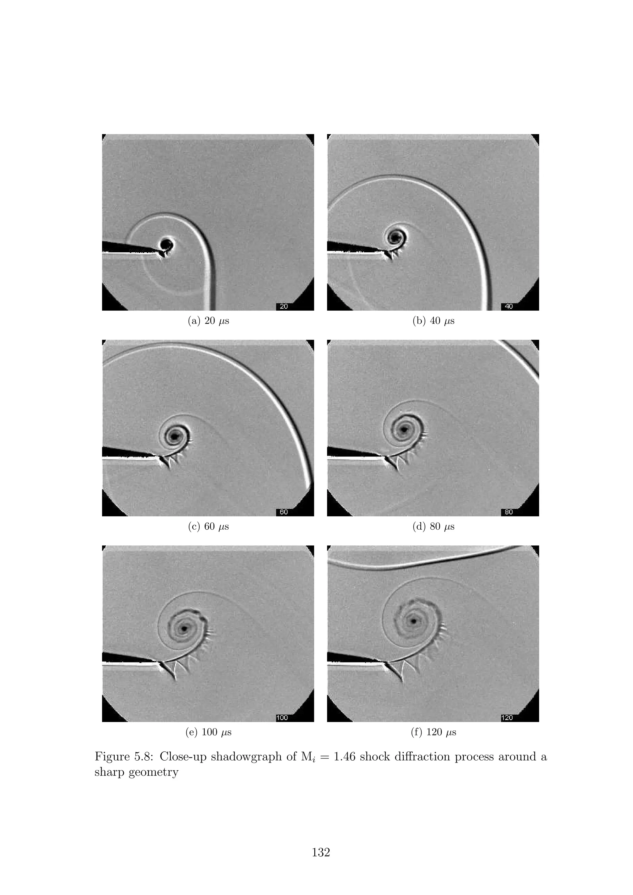
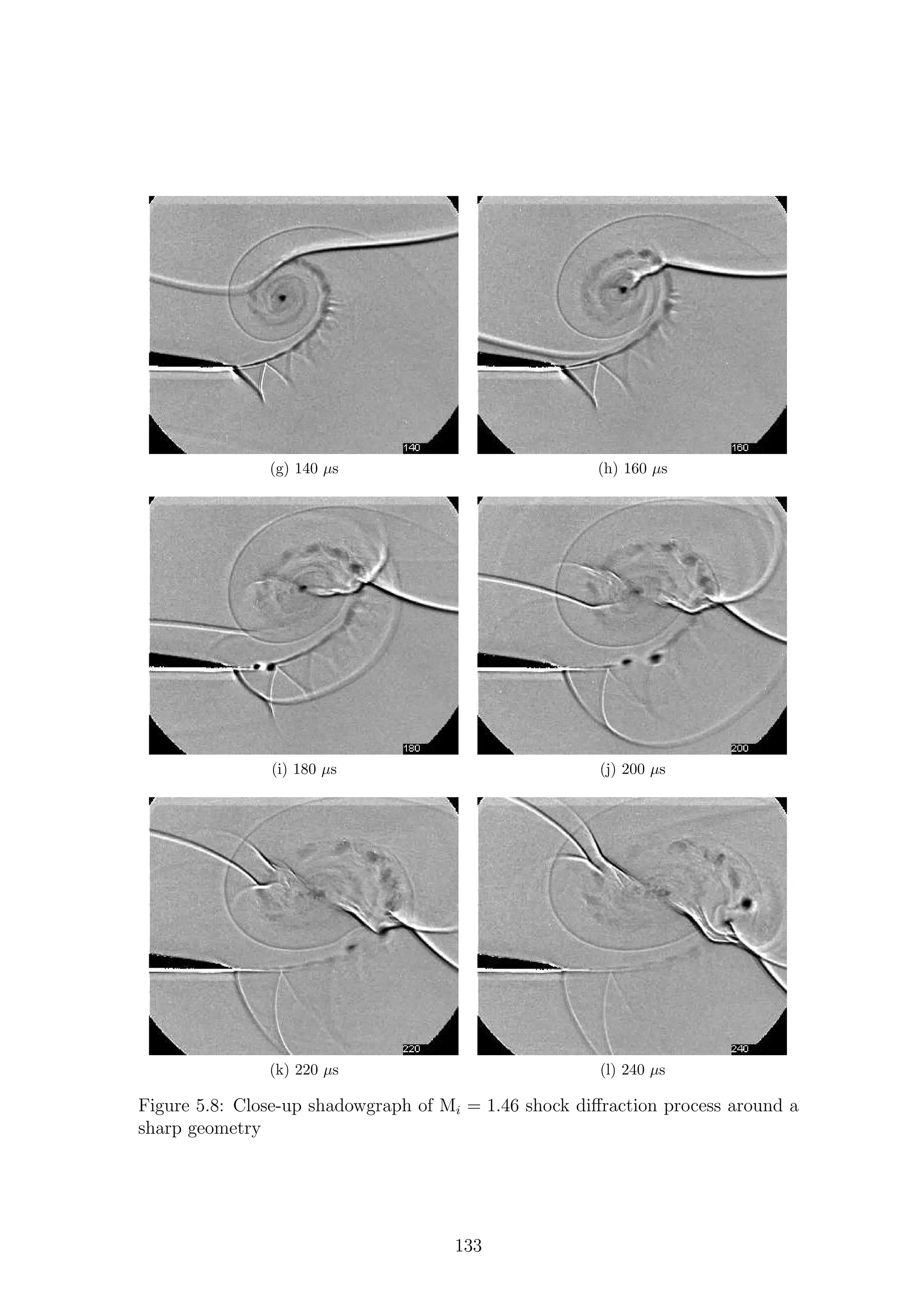
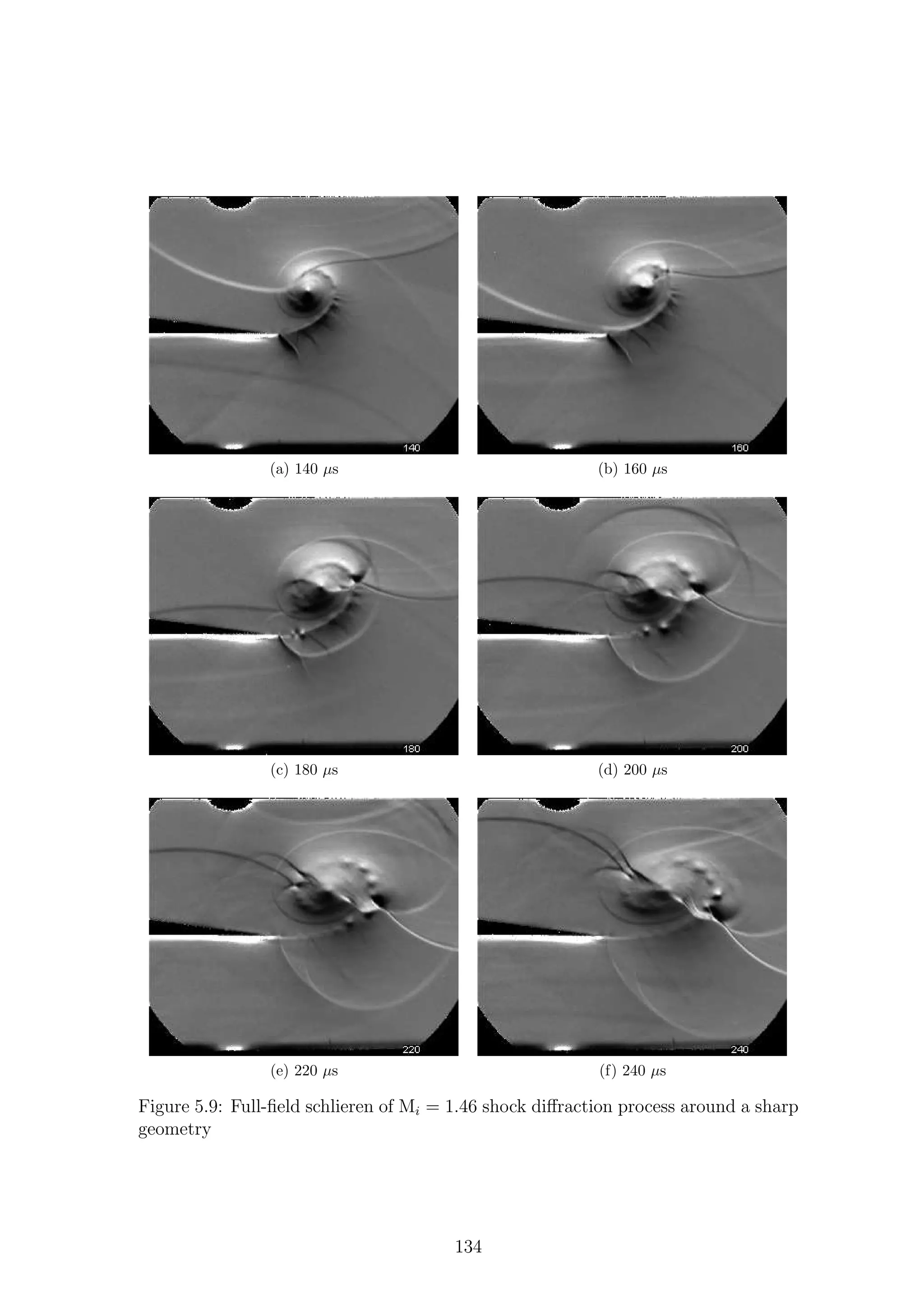
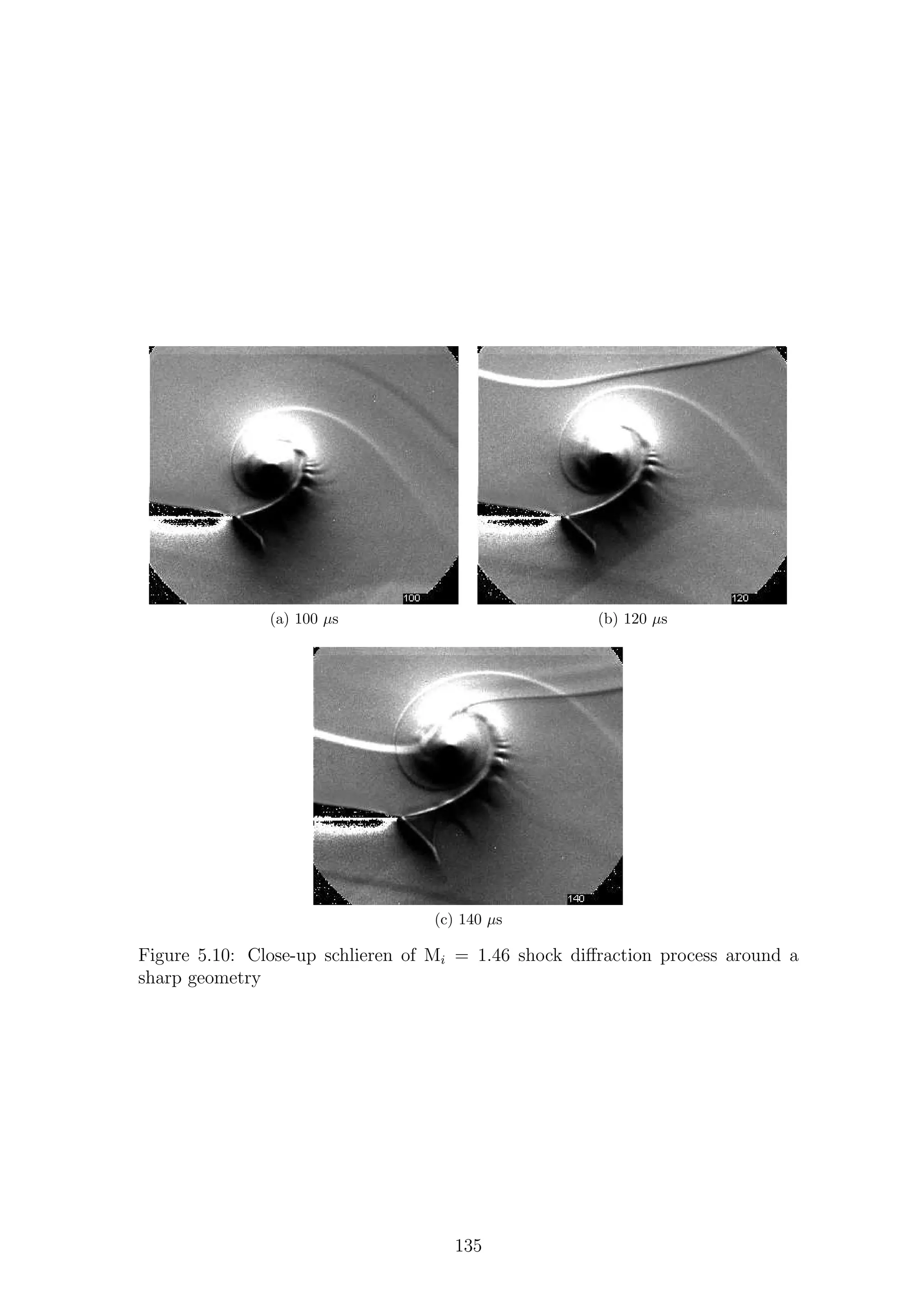
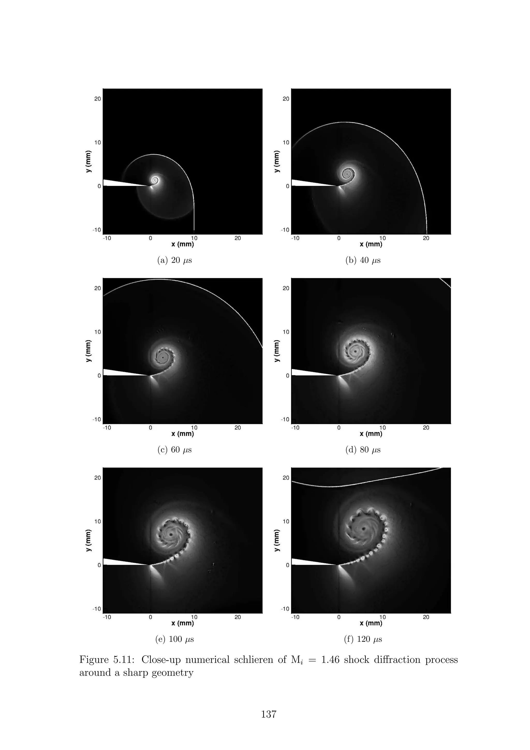
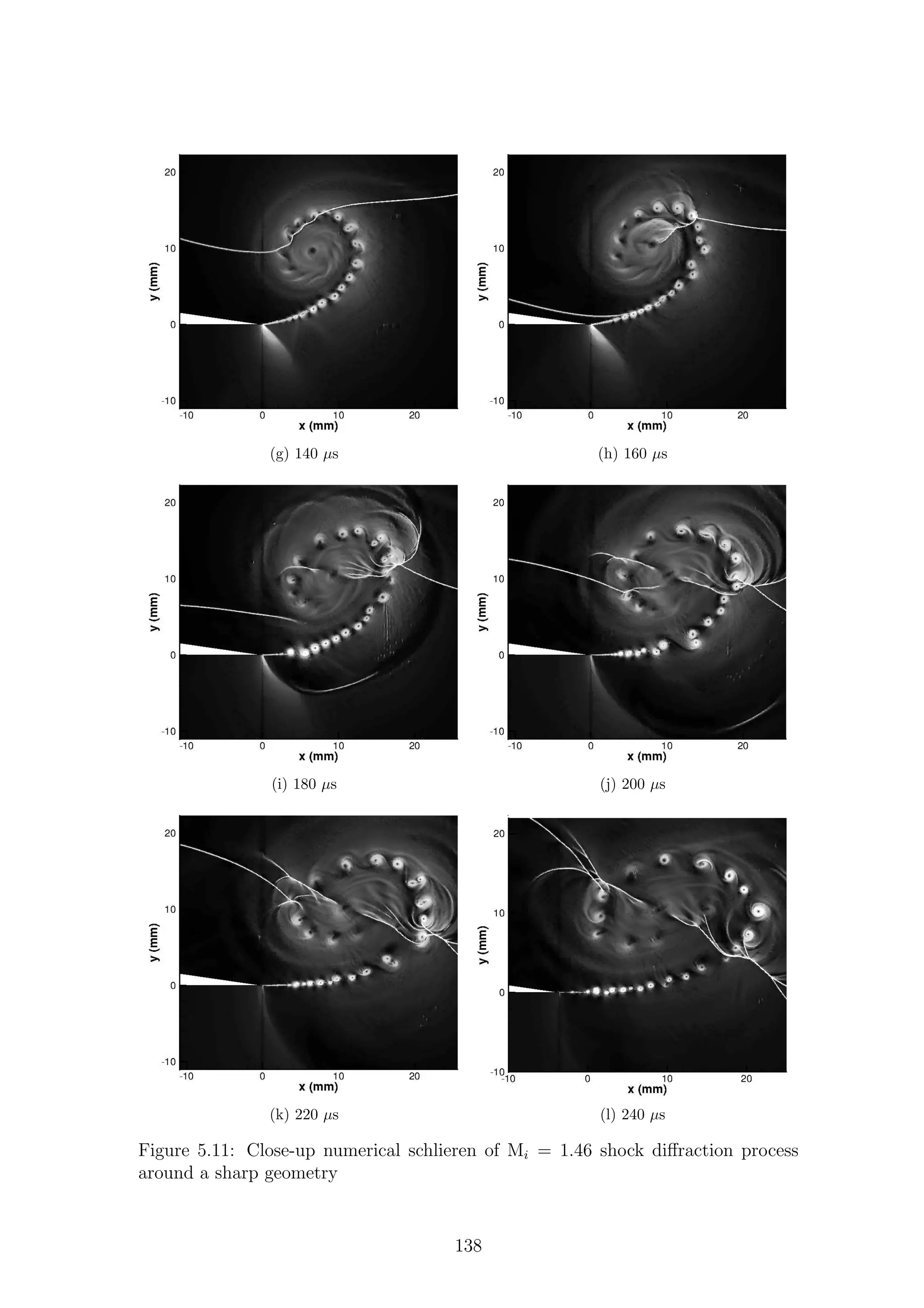
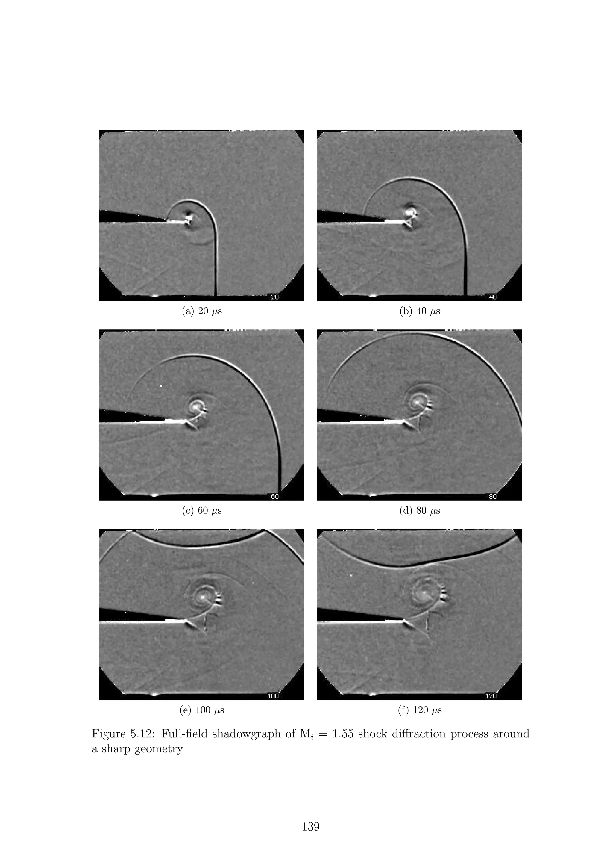
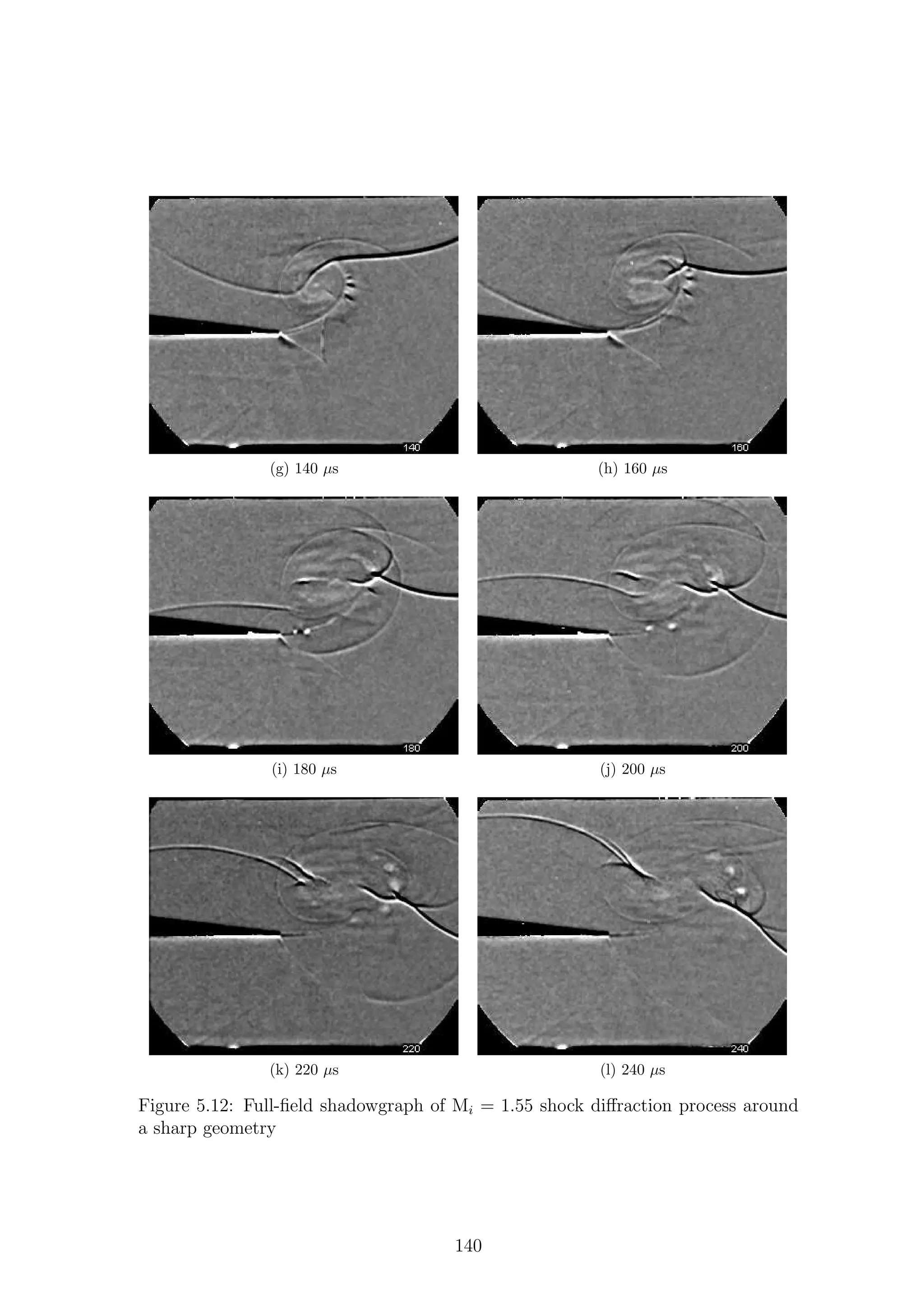
![Examining Fig.5.14f more closely, we can see that there are no apparent distur-
bances on the shear layer until the end of the structures seen on the outside of it
(approximately 100◦
around the vortex). After this point, there are structures which
can faintly be seen on the shear layer, suggesting that the K-H instability is more
heavily damped in regions where one side of the shear layer has localised supersonic
flow. Such a result is in accordance of the work of Papamoschou & Roshko [52] and
Miles [1].
The embedded shock wave can partially be seen in Figs.5.13d to 5.13g, but is
more clearly seen in Fig.5.14, specifically in Figs.5.14f & 5.14g. The shear layer
in the vortex roll-up process can be thought of as a solid line which fluid cannot
pass over. The main vortex induces velocity above the shear layer and the figures
clearly show that the shear layer rolls up around the vortex. If the shear layer can be
thought of as a boundary, then the fluid in this region is passing through a reduction
in area and could be accelerated up to sonic speeds. This acceleration will come
hand-in-hand with a reduction in pressure. Therefore, a shock wave is required to
balance the pressure on either side of the shear layer.
Figs.5.13k & 5.13l show that, after the passage of the returning shock wave
through the shear layer, there are some disturbances present on the shear layer,
indicating the early stages of a further K-H instability. Instabilities which passed
down the shear layer at this point are broken up into patches of turbulence by the
shock vortex interaction, as can be seen on the far right of Figs.5.13k & 5.13l. The
centre of the main vortex also displays the properties of a strong patch of turbulence.
Fig.5.13l shows that the main vortex has been severely distorted by the passage of
the returning diffracted shock wave. The vortex has been stretched in the horizontal
direction, giving it an elliptical shape.
5.1.1.6 Mi = 1.55 Numerical Results
The numerical schlieren results for Mi=1.55 are presented in Figs.5.16 & 5.17. The
basic wave structure is well captured, so the main focus will be on the complex
region.
Similar to the previous case, shown in Fig.5.11, the lambda structures below the
shear layer are not well defined by the simulation. Figs.5.16b to 5.16d show the
first and second lambda structure, but after this time the second one becomes more
and more diffuse. The vortex shock seen in the experimental results is captured,
although it does not seem to extend as far as the shear layer. It is interesting to
note that the wave structures seen on the outside of the shear layer (90◦
around the
vortex in Fig.5.16b onwards) appear to have been resolved, even though the lambda
structures leading up to them have not. This suggests that the structures are not a
continuation of the lambda shocks, but are, in fact, a function of something else.
The instability of the shear layer appears to be overpredicted in the numerical
results, as there was little indication from Figs.5.12, 5.13 & 5.14 that so many
vortices were produced so quickly.
The shock-vortex interaction shown in the latter images of Fig.5.16 and Fig.5.17
proceeds in a very similar manner to the experiments. The impact of the returning
shock generates the two strong vortices, which immediately begin to pull another,
weaker, vortex around them. As in the previous numerical cases, a secondary K-
H instability is generated. This instability develops much more quickly than the
141](https://image.slidesharecdn.com/4a6f74b5-6bbb-4ffd-b3f5-7486cdb057cd-150303082443-conversion-gate01/75/Mark-Quinn-Thesis-172-2048.jpg)
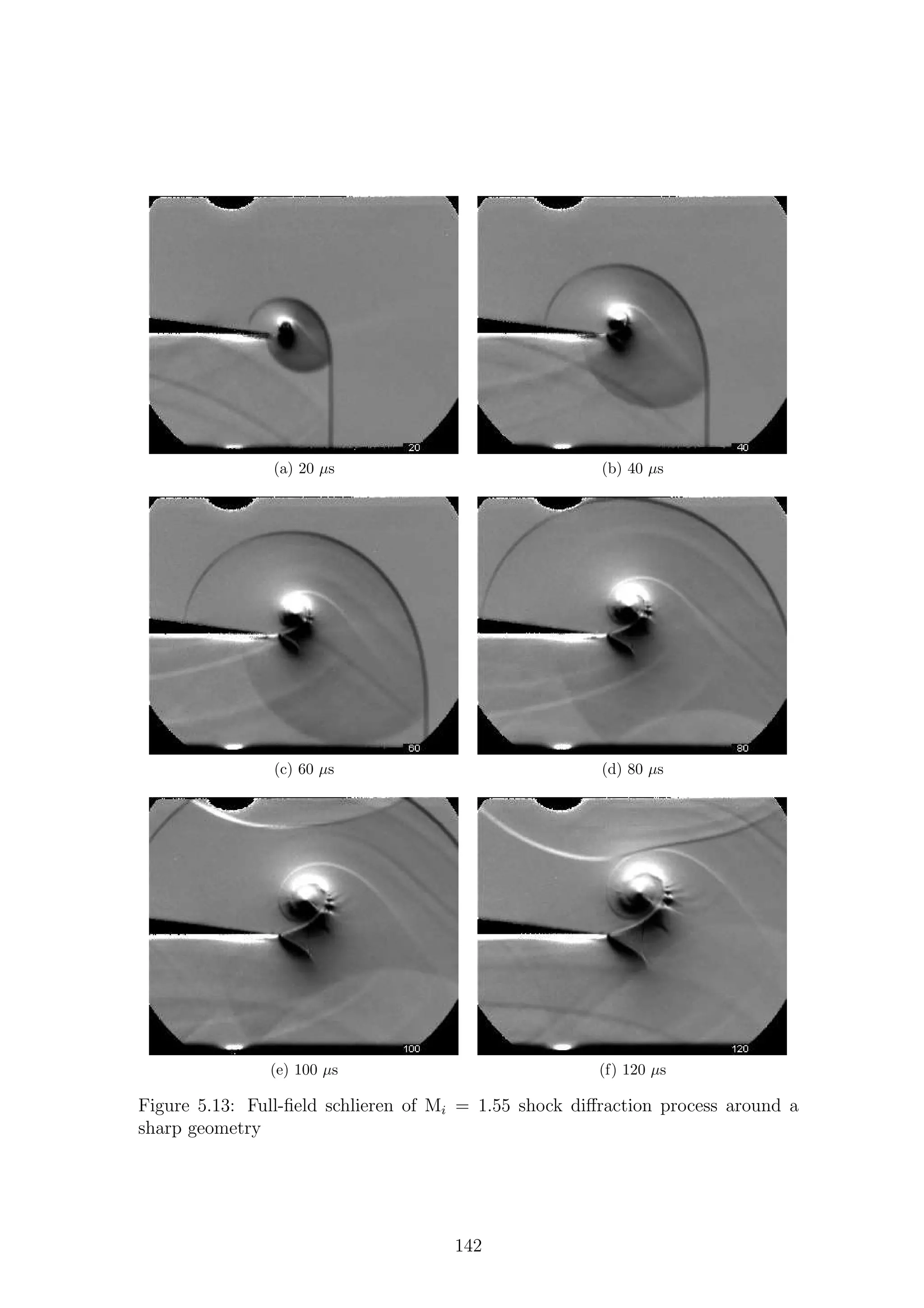
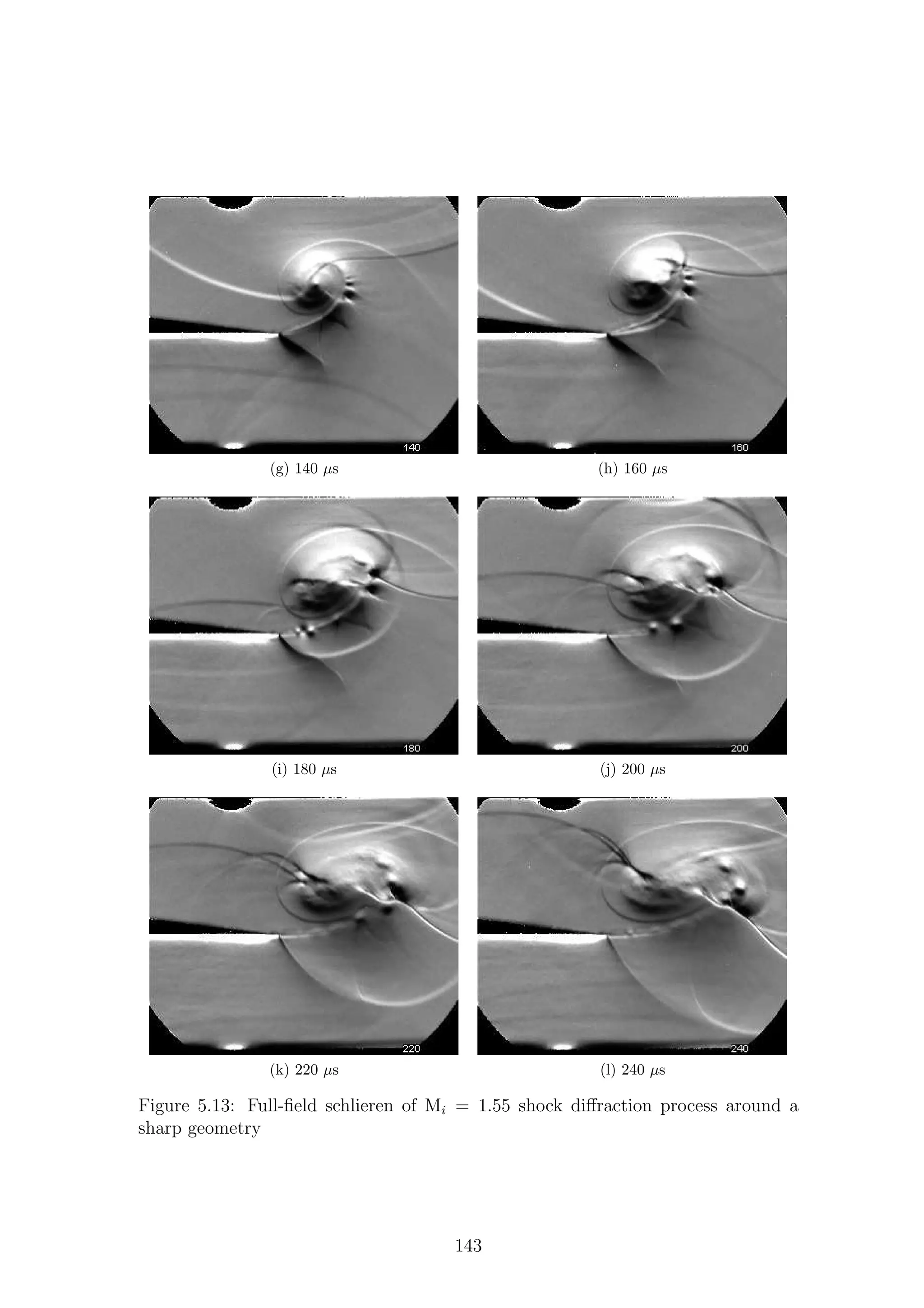
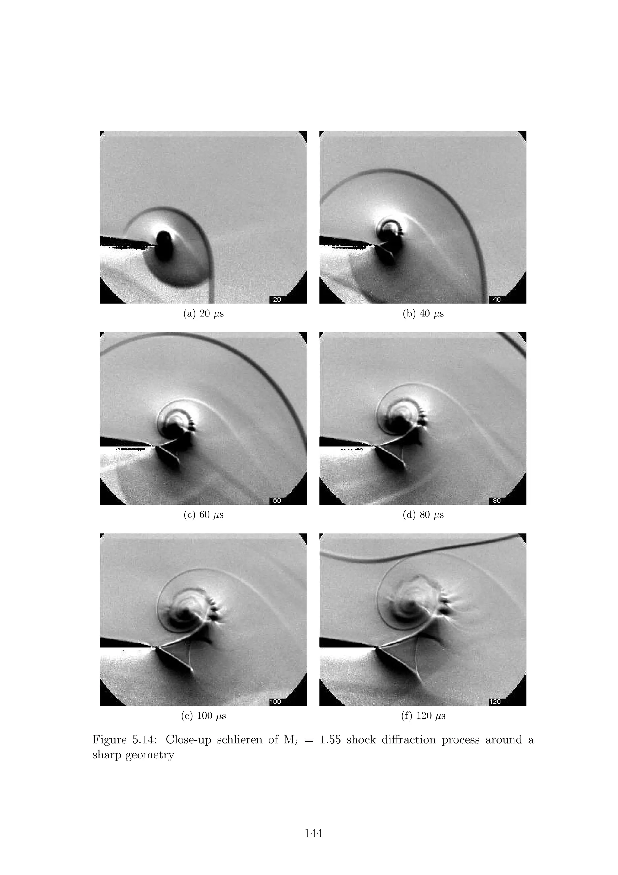
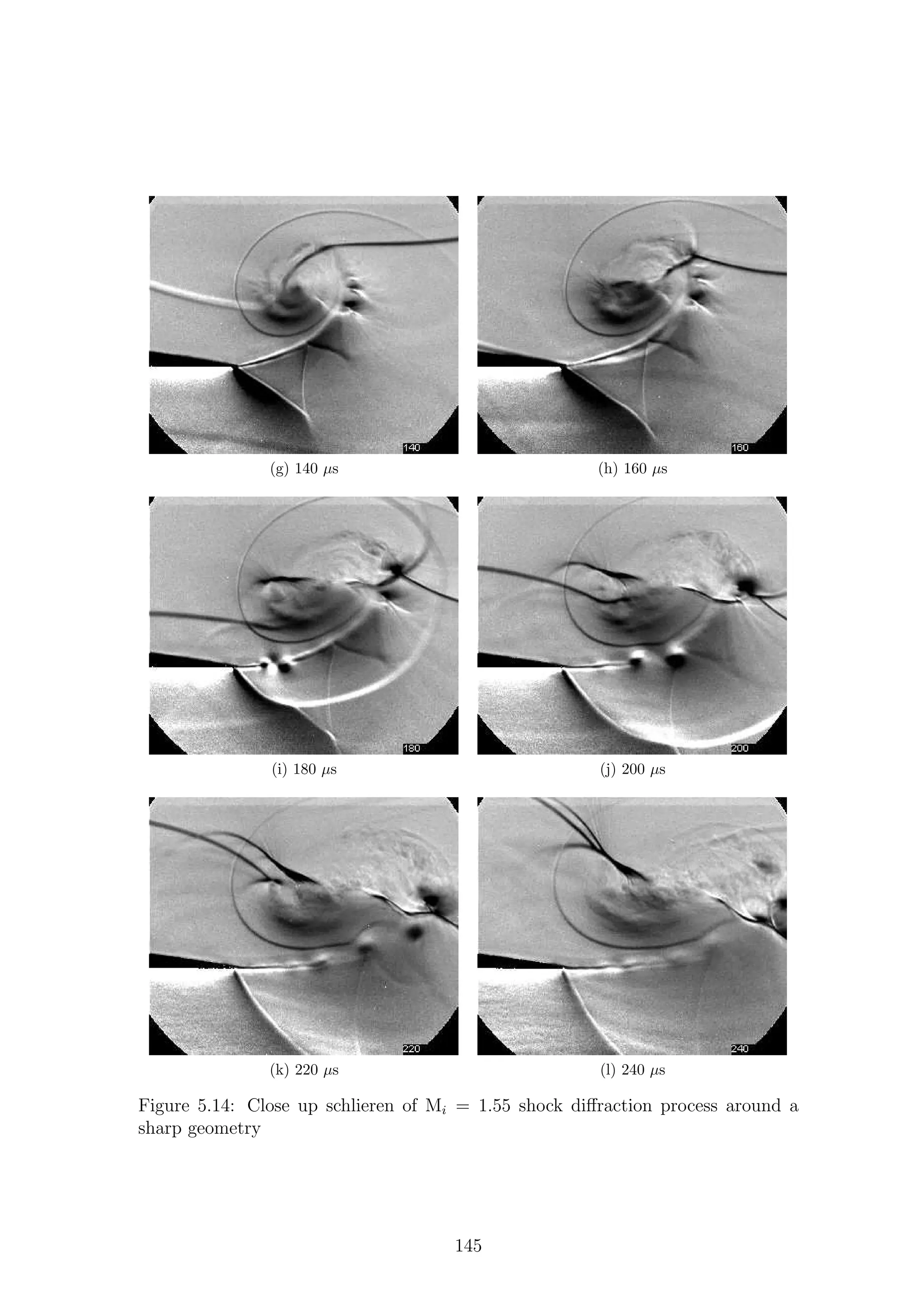
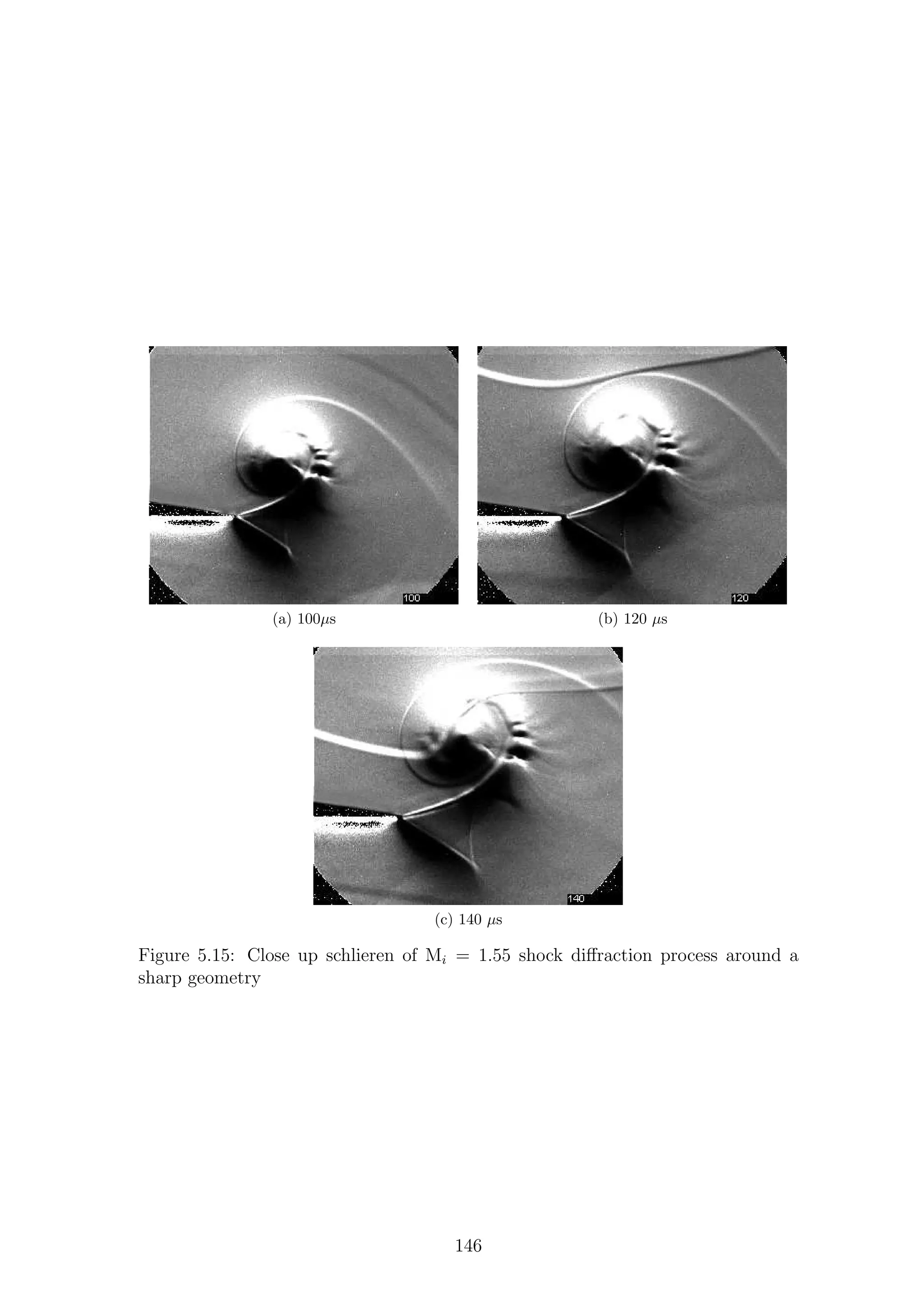
![experimental disturbances seen in Figs.5.14k & 5.14l.
5.1.1.7 Conclusions
The process of shock wave diffraction around a sharp corner has been studied using
a variety of optical setups. The shock wave systems generated are different over a
relatively narrow range of incident Mach numbers. A Mi = 1.28 does not generate
any visible lambda structures underneath the shear layer, leading to the conclusion
that the flow in this region is entirely subsonic. This is consistent with the criti-
cal Mach number theory presented by Sun & Takayama [36]. Both of the higher
Mach number cases (Mi = 1.46 and Mi = 1.55) show a series of lambda struc-
tures underneath the shear layer in the expansion region. The Mi = 1.46 case shows
many small lambda structures which eventually degenerate into structures too small
to distinguish; however, the Mi = 1.55 shows a significantly larger initial lambda
structure with fewer subsequent lambda structures. This leads to the conclusion
that the flow is tending towards the strong shock solution presented in Fig.2.12c.
The contact surface between the gas affected by the normal shock compared to the
curved, diffracted portion, is swept up into the main vortex.
The results in this section show that the instabilities present on the shear layer
created during shock wave diffraction can only be clearly seen by using a focused
shadowgraph system with a shallow depth of field in conjunction with an ultra-high-
speed camera. Previous experimental tests have only been conducted using schlieren
or one shadowgraph setup. Schlieren systems are easily overranged, especially in the
region of the main vortex, as the density changes in this region are especially strong,
leading to some flow features being missed.
The shear layer created in this experiment is extremely thin, due to the nature
of the corner geometry. The shear layer is so thin that it is almost impossible to
accurately estimated its width given the limited spatial resolution. This thin shear
layer is closer to the vortex sheet approximation made in Section 2.5 than in other
work, such as that by Skews [32]. This thinner shear layer can act in a more inviscid
manner than the thicker ones generated by shallower corner angles and can rapidly
develop instabilities. Other tests, such as the 90◦
corner, will generate instabilities
eventually, such as those seen by Skews [33]. An increase in incident shock Mach
number seems to inhibit the growth of the instabilities, especially around the lambda
structure region where the flow is locally supersonic on one side of the shear layer.
It is a known phenomena that as the velocity ratio increases across a shear layer,
particularly to a locally supersonic speed, instabilities can be damped out. Further
to this, the majority of work performed on this problem involves using a 90◦
corner
as the test geometry. In these tests the vortex is in such close proximity to the wall,
that a wall shock formed. This will compress the flow in this region, thus increasing
its density. If the density on the low-speed side of the shear layer is higher, the
flow is less susceptible to small wavelengths, as the complex part of Equation 2.55
is smaller.
The diffraction process appears to be self-similar in time, with the exception of
the shear layer instabilities. The instabilities on the shear layer will take a finite
time to develop and as a result the flow cannot be considered completely self-similar
in time.
The interaction of the cylindrical diffracted shock wave and the main vortex
147](https://image.slidesharecdn.com/4a6f74b5-6bbb-4ffd-b3f5-7486cdb057cd-150303082443-conversion-gate01/75/Mark-Quinn-Thesis-178-2048.jpg)
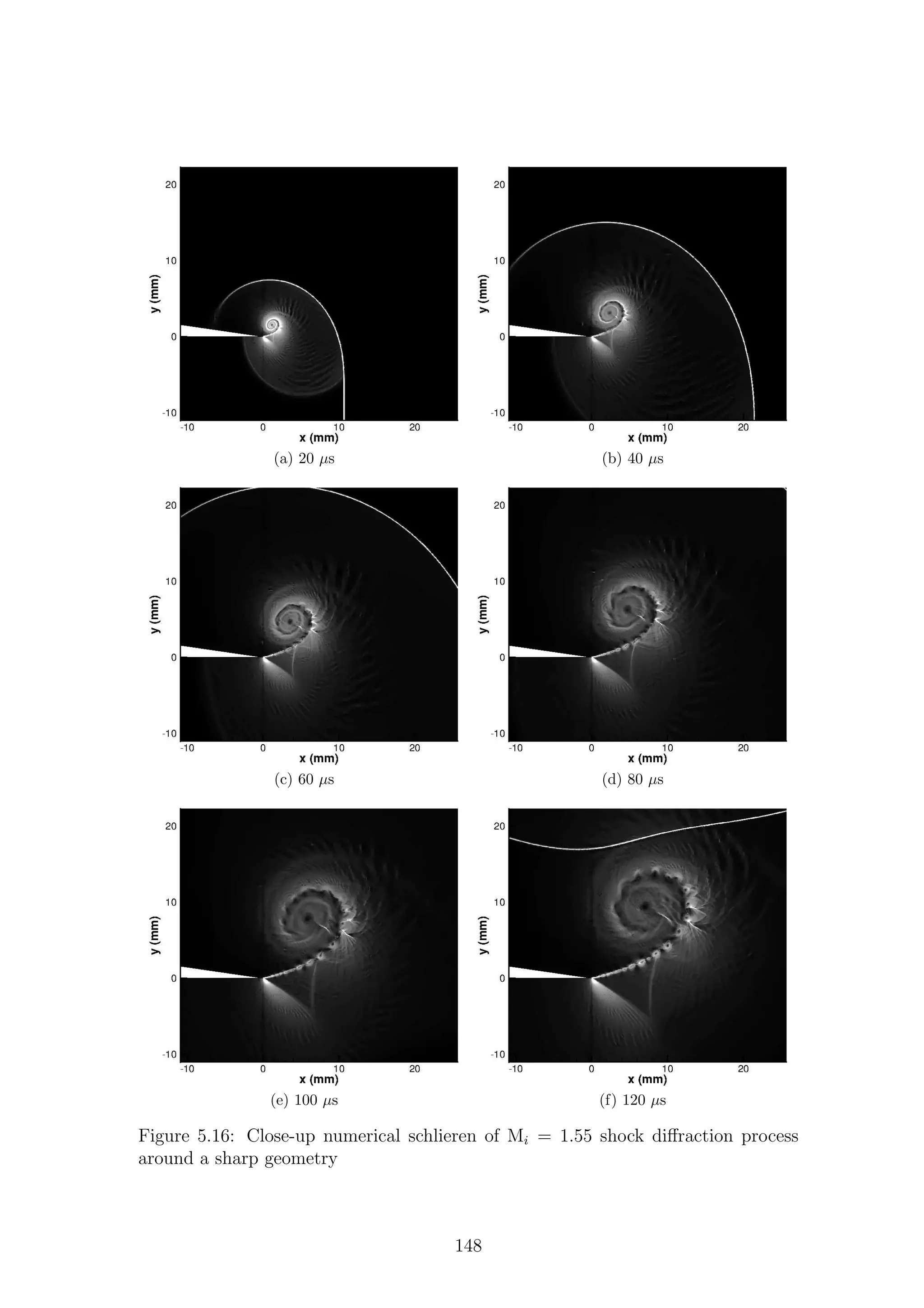
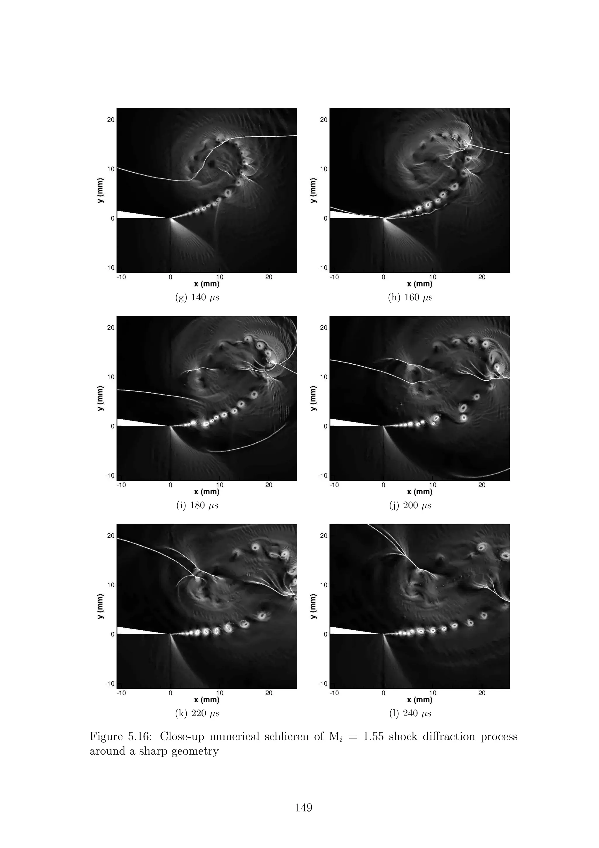
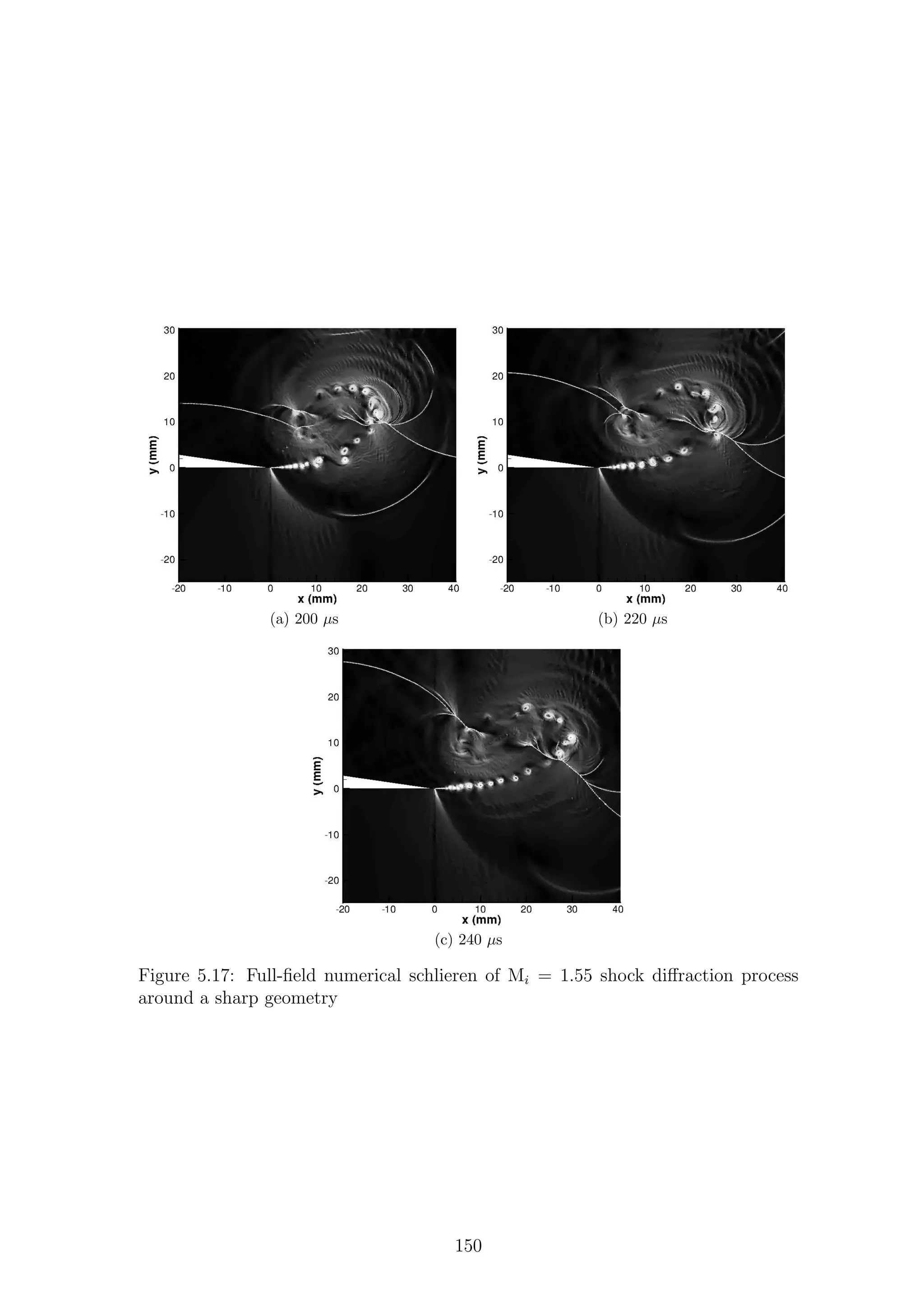
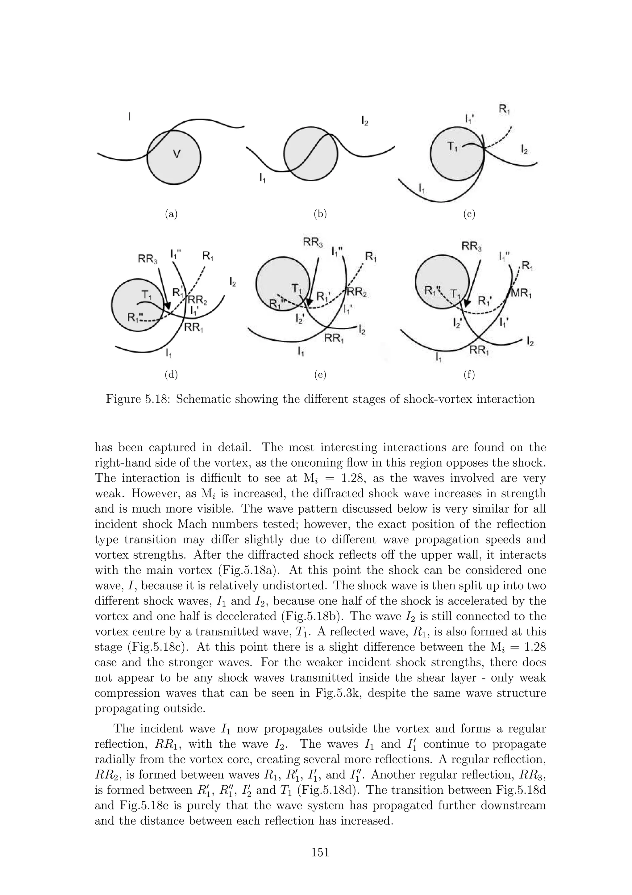
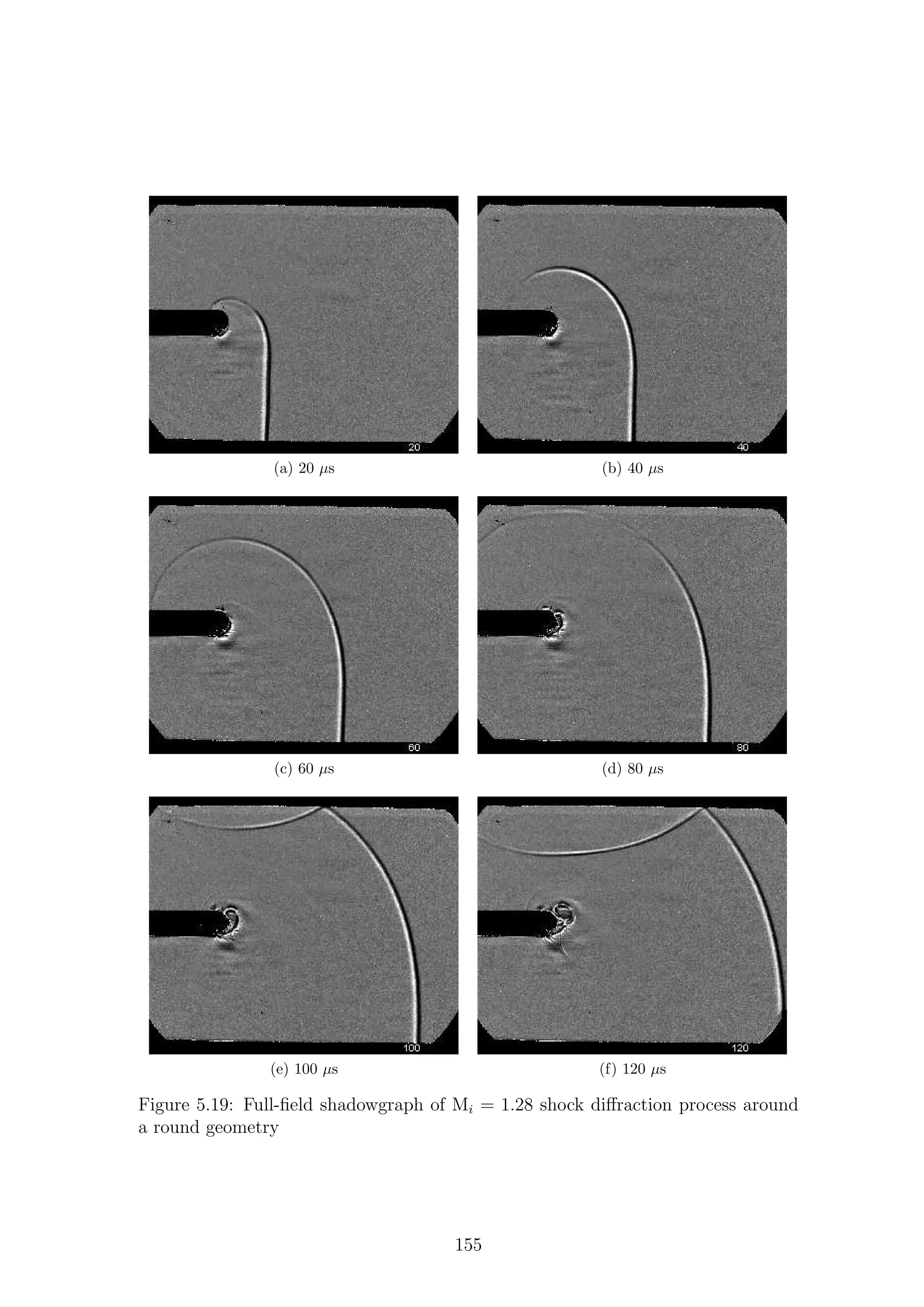
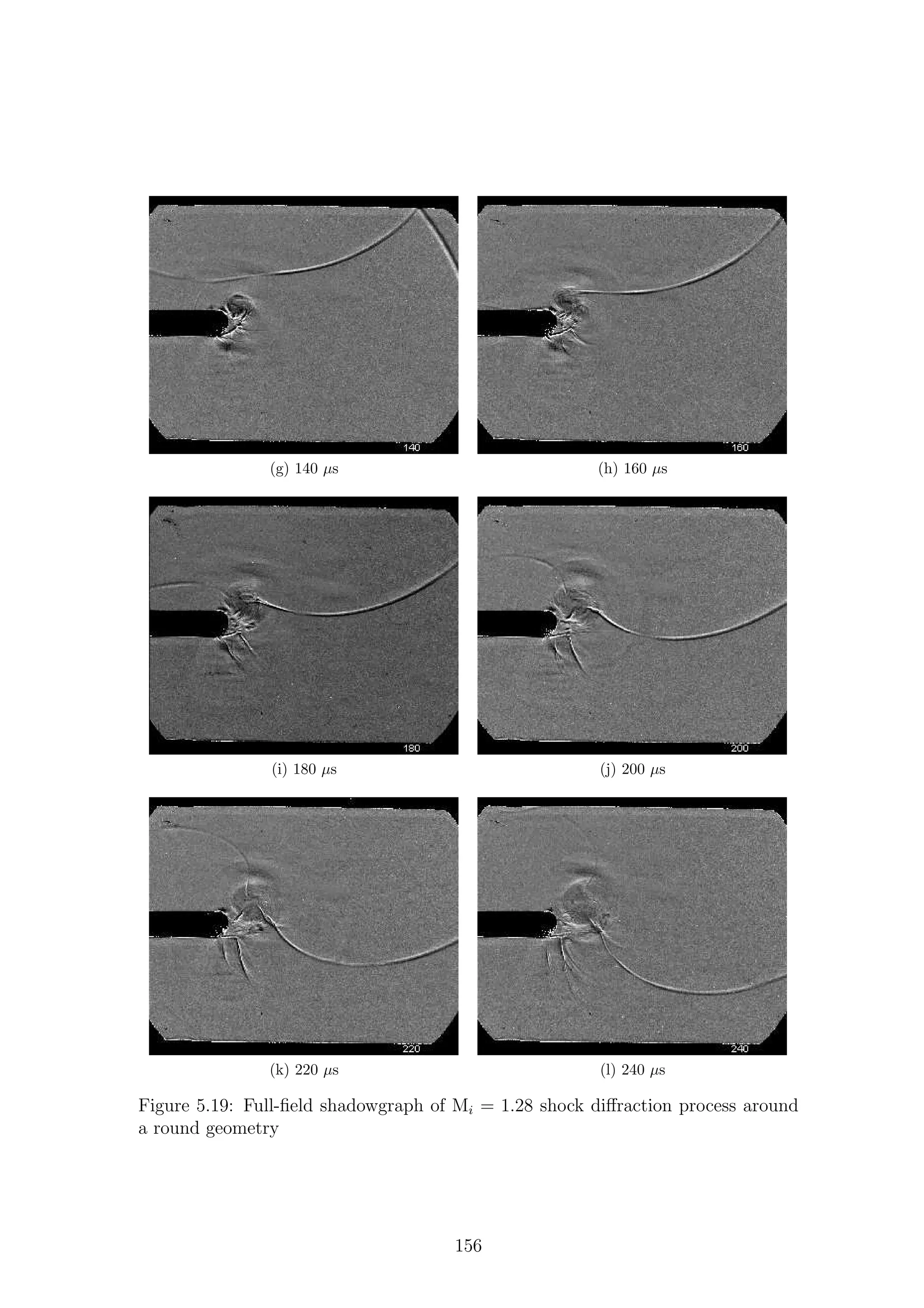
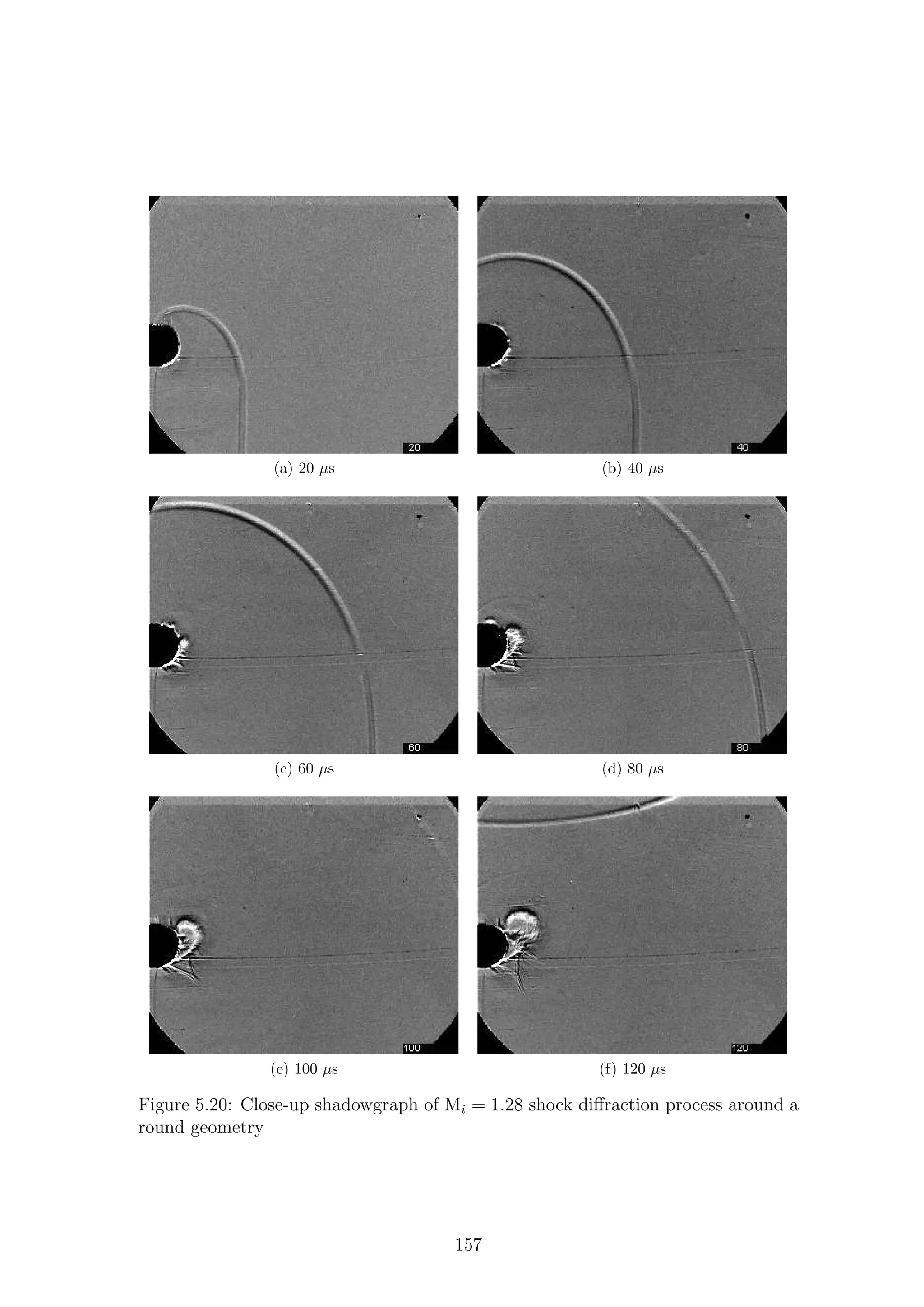
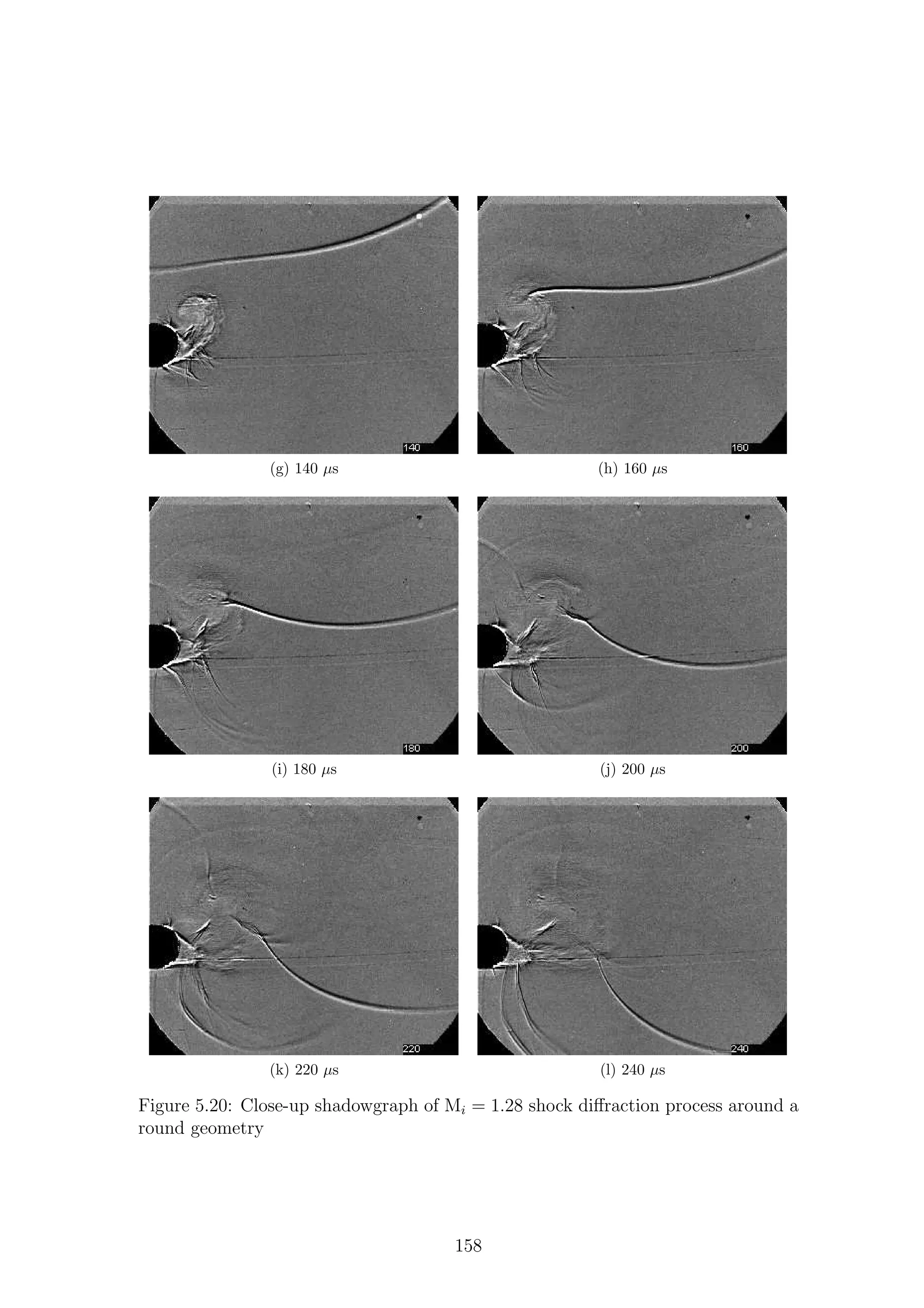
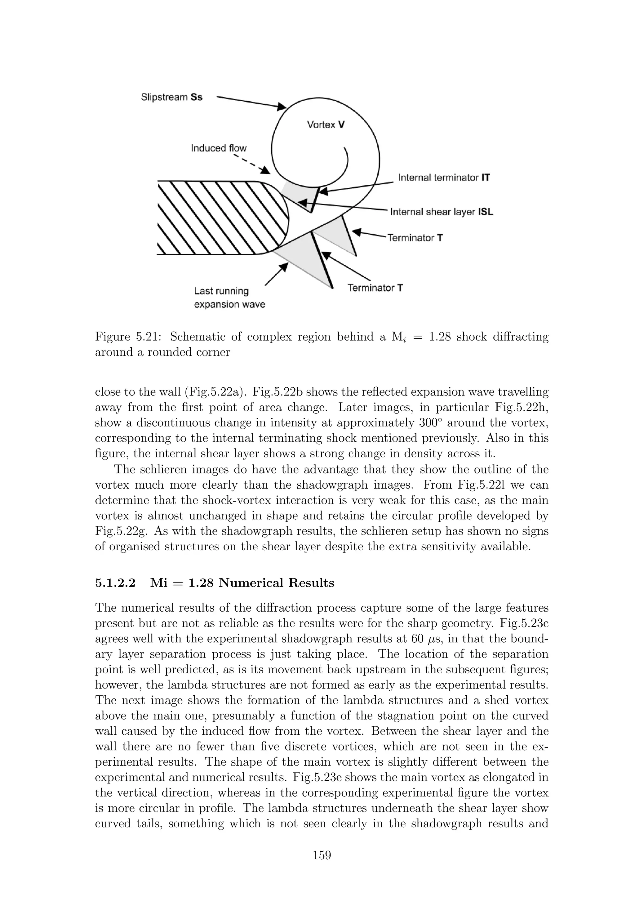
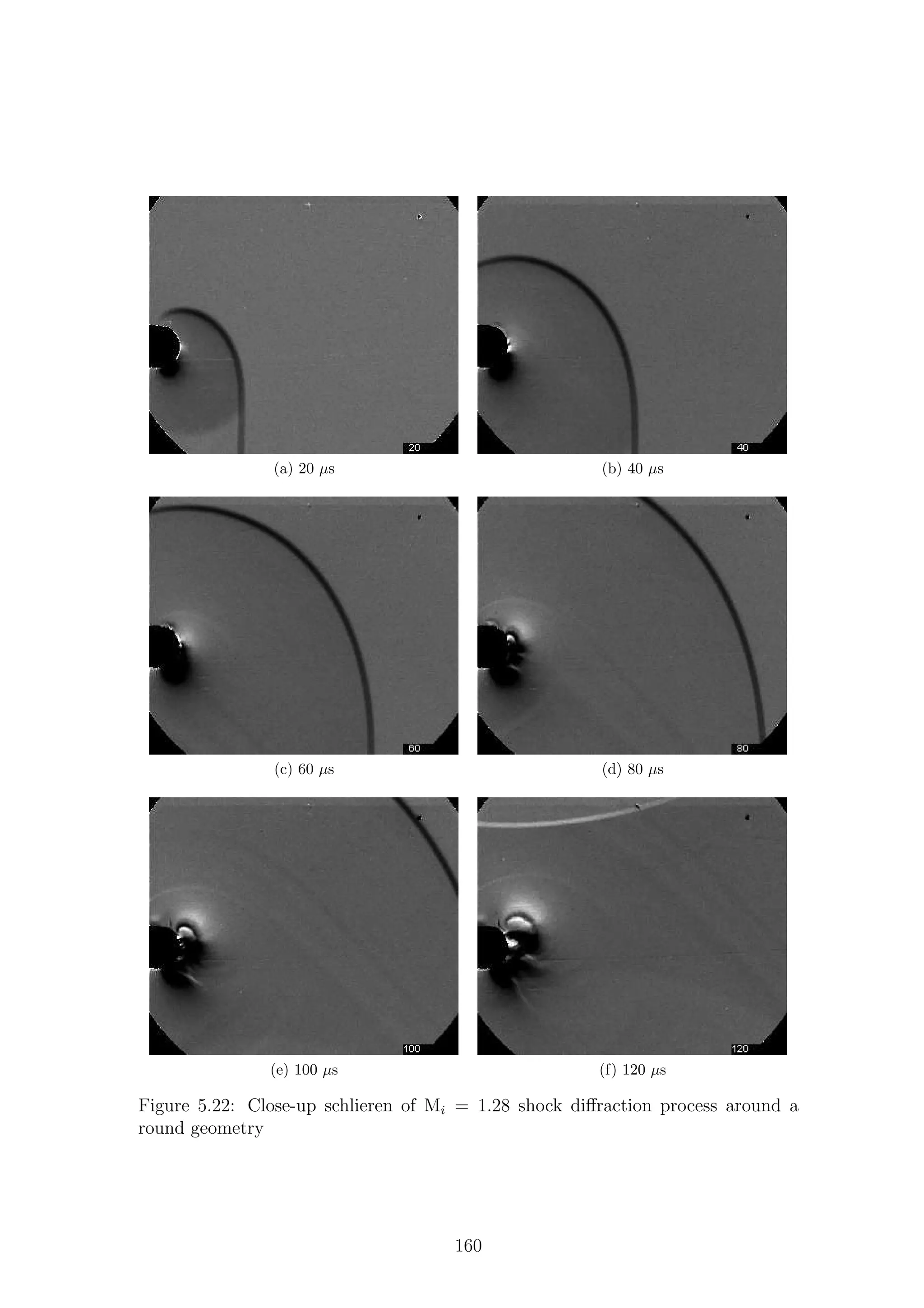
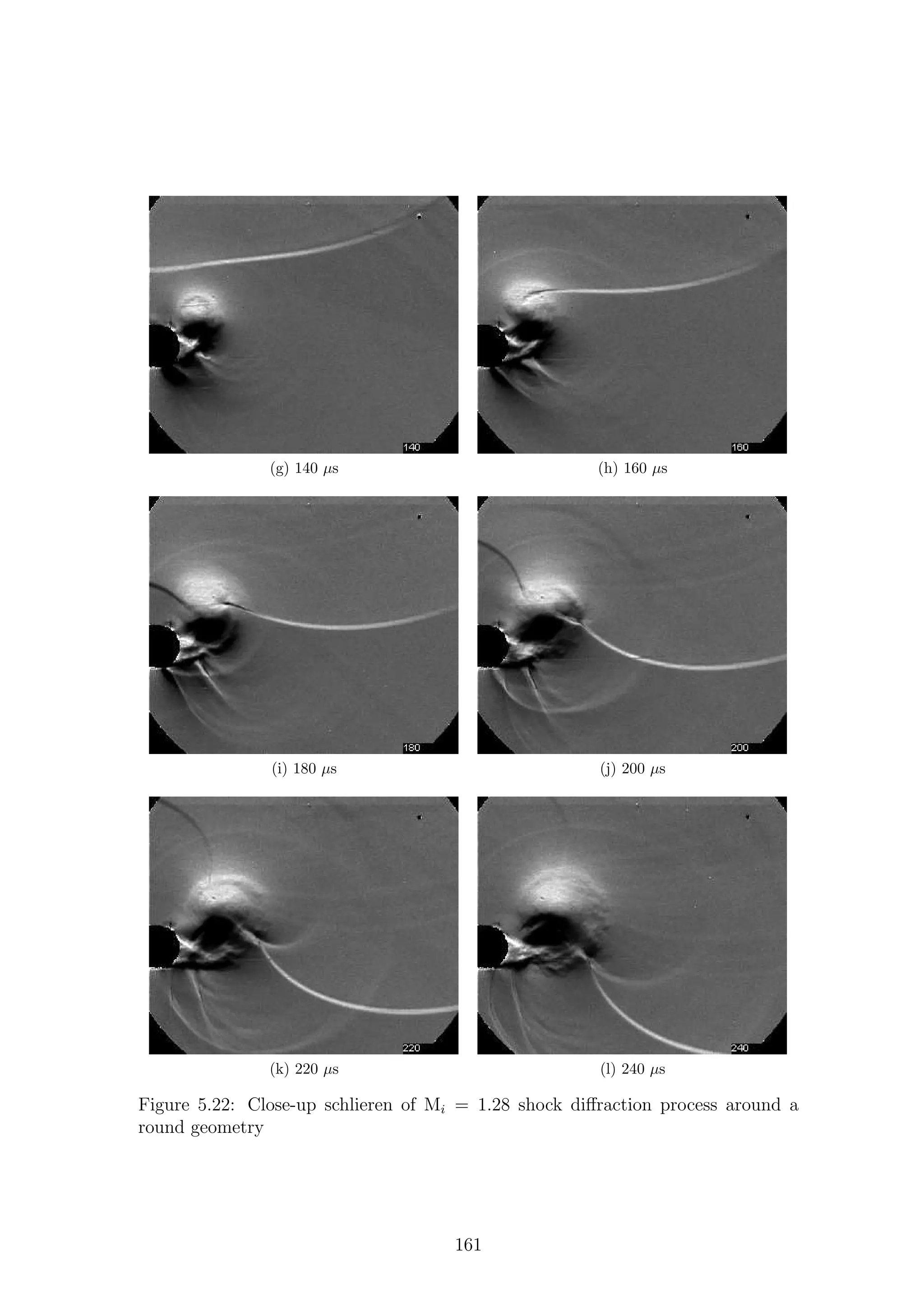
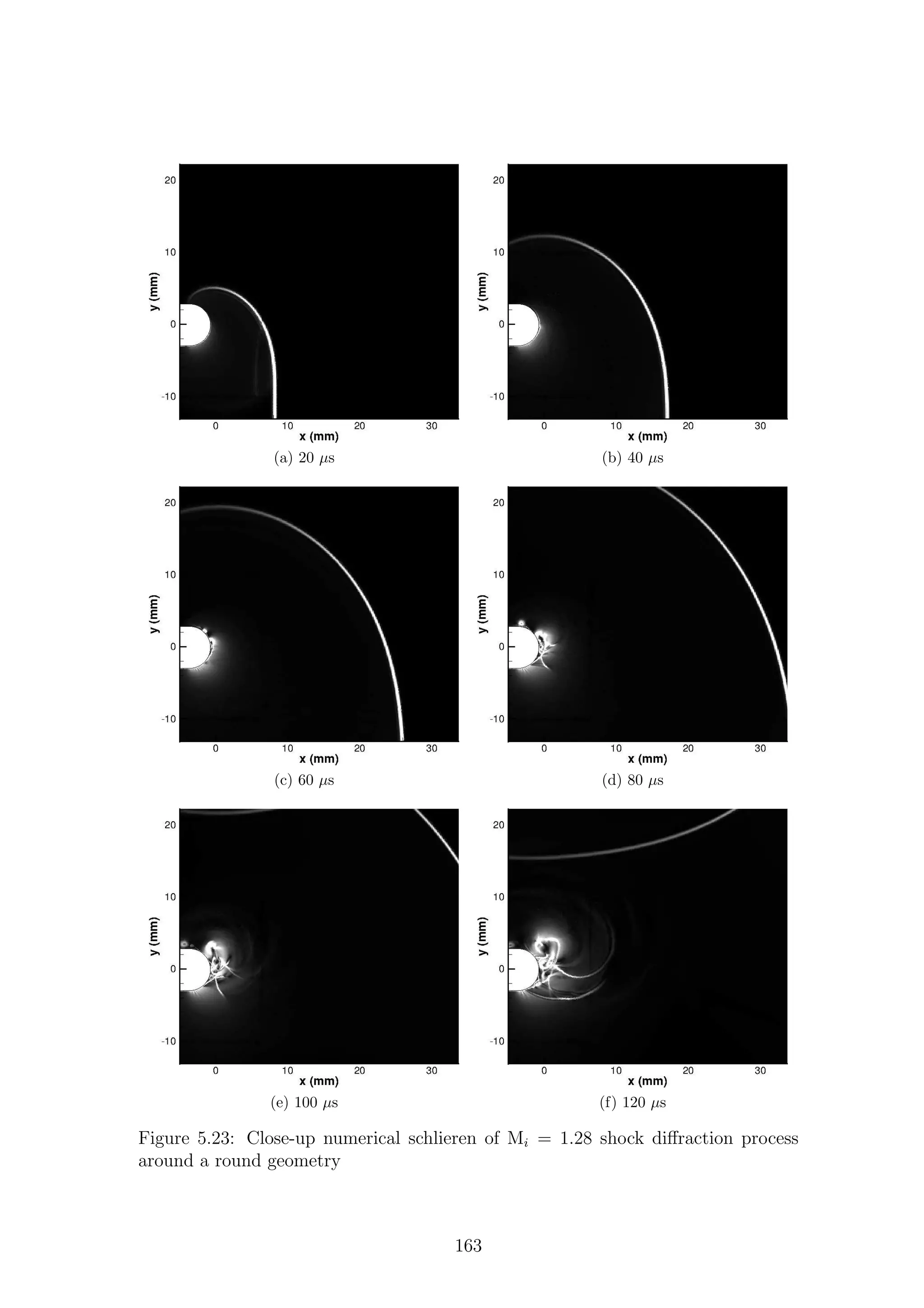
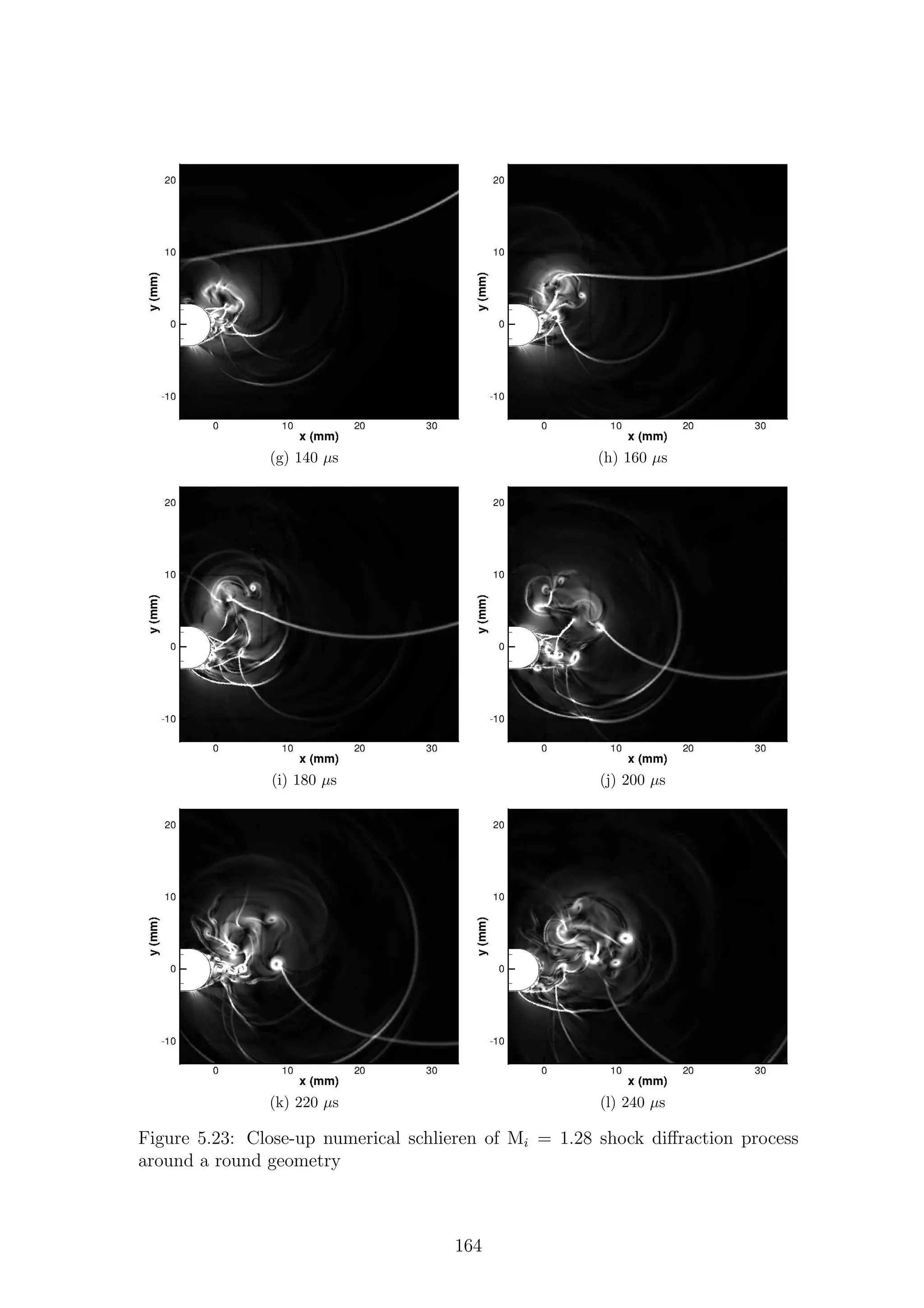
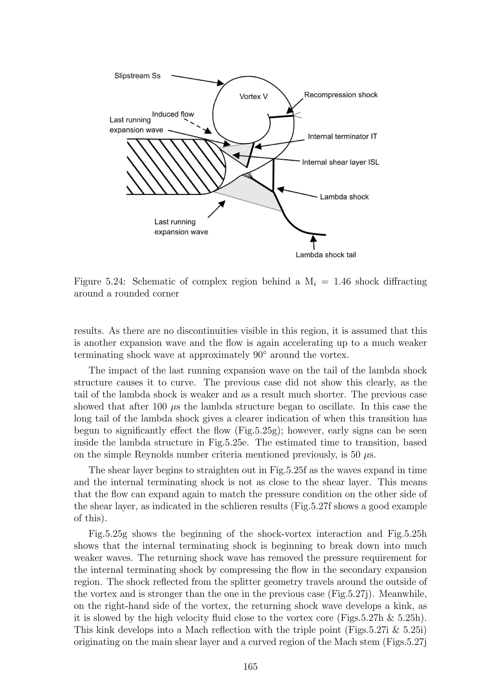
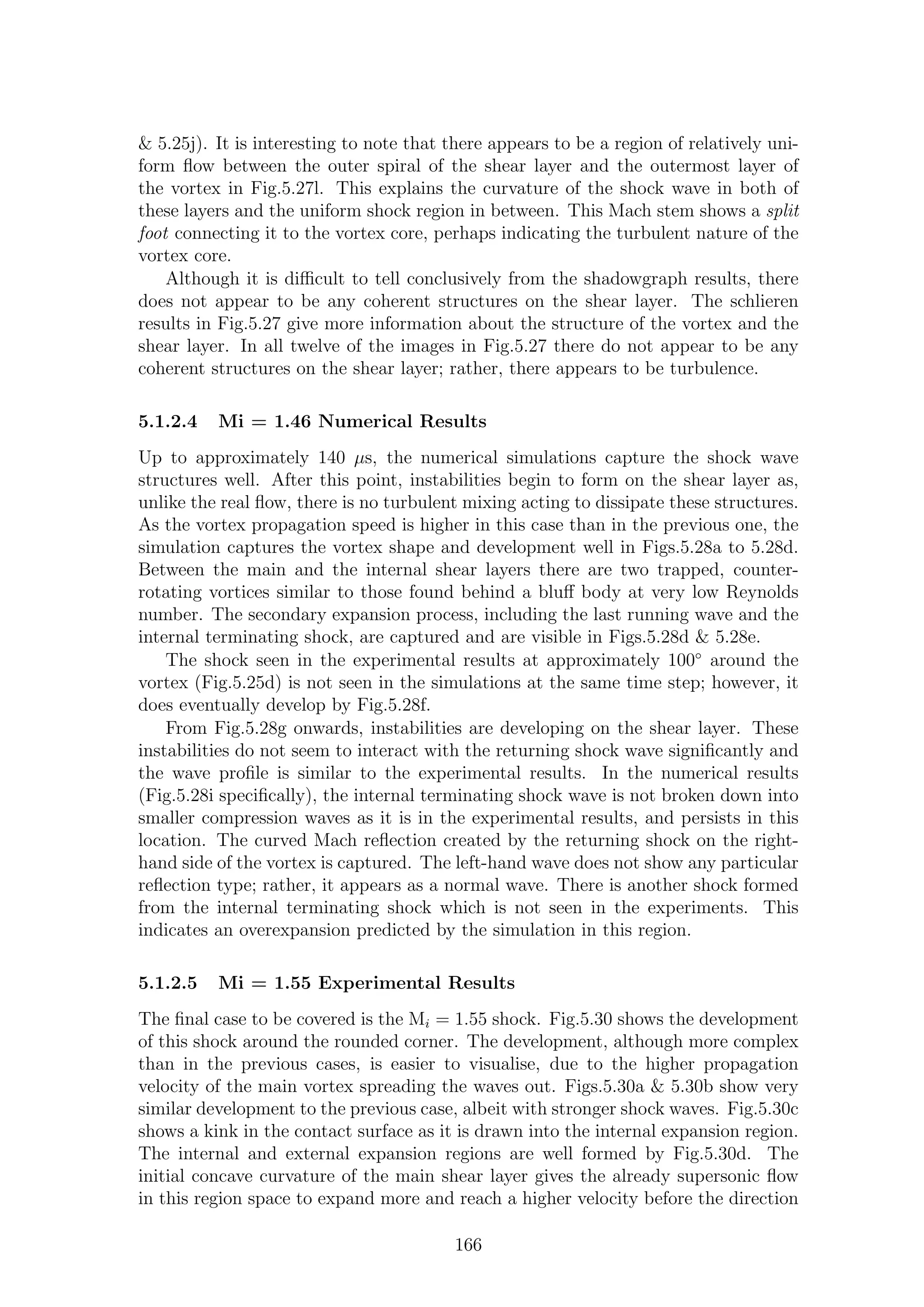
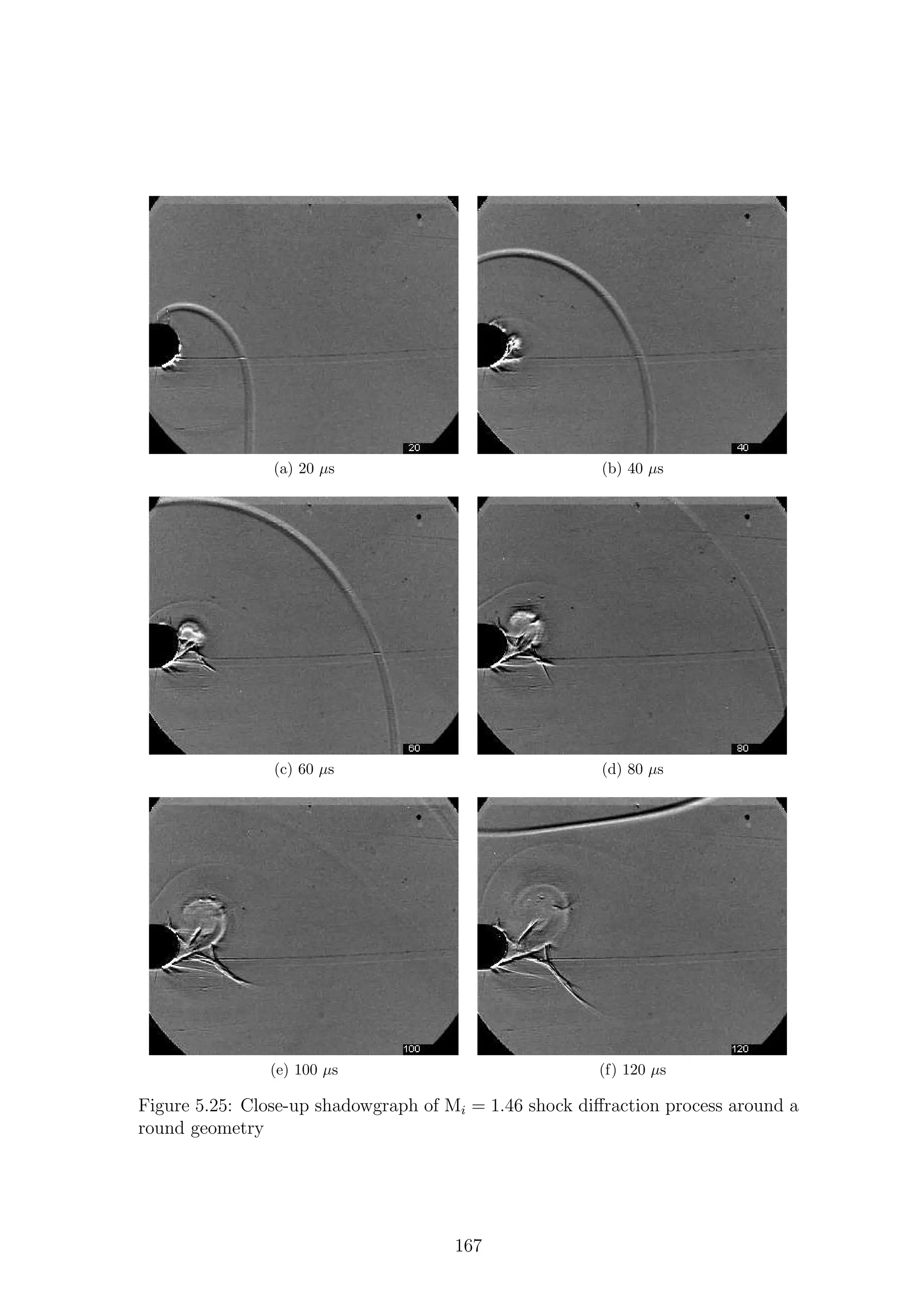

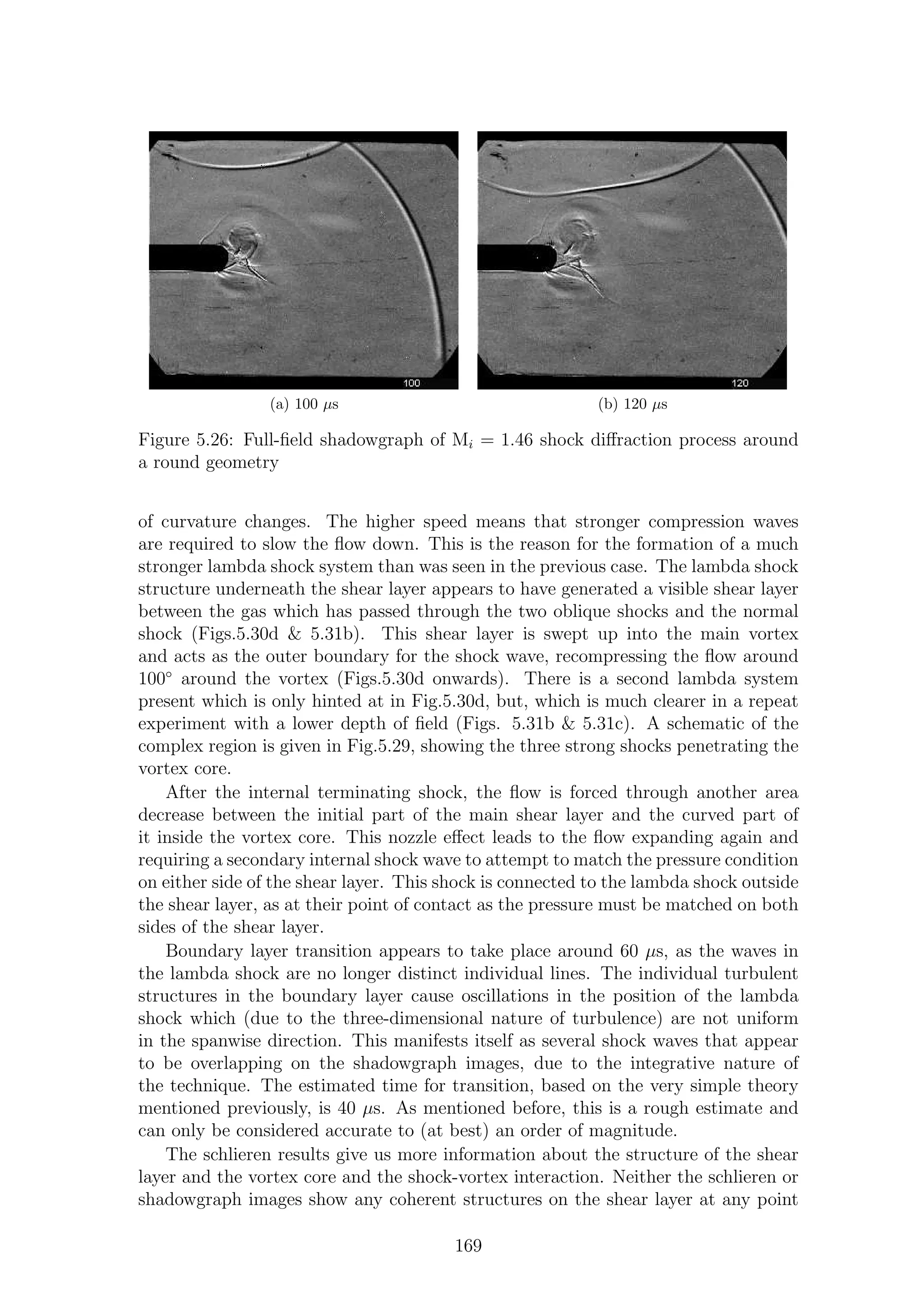
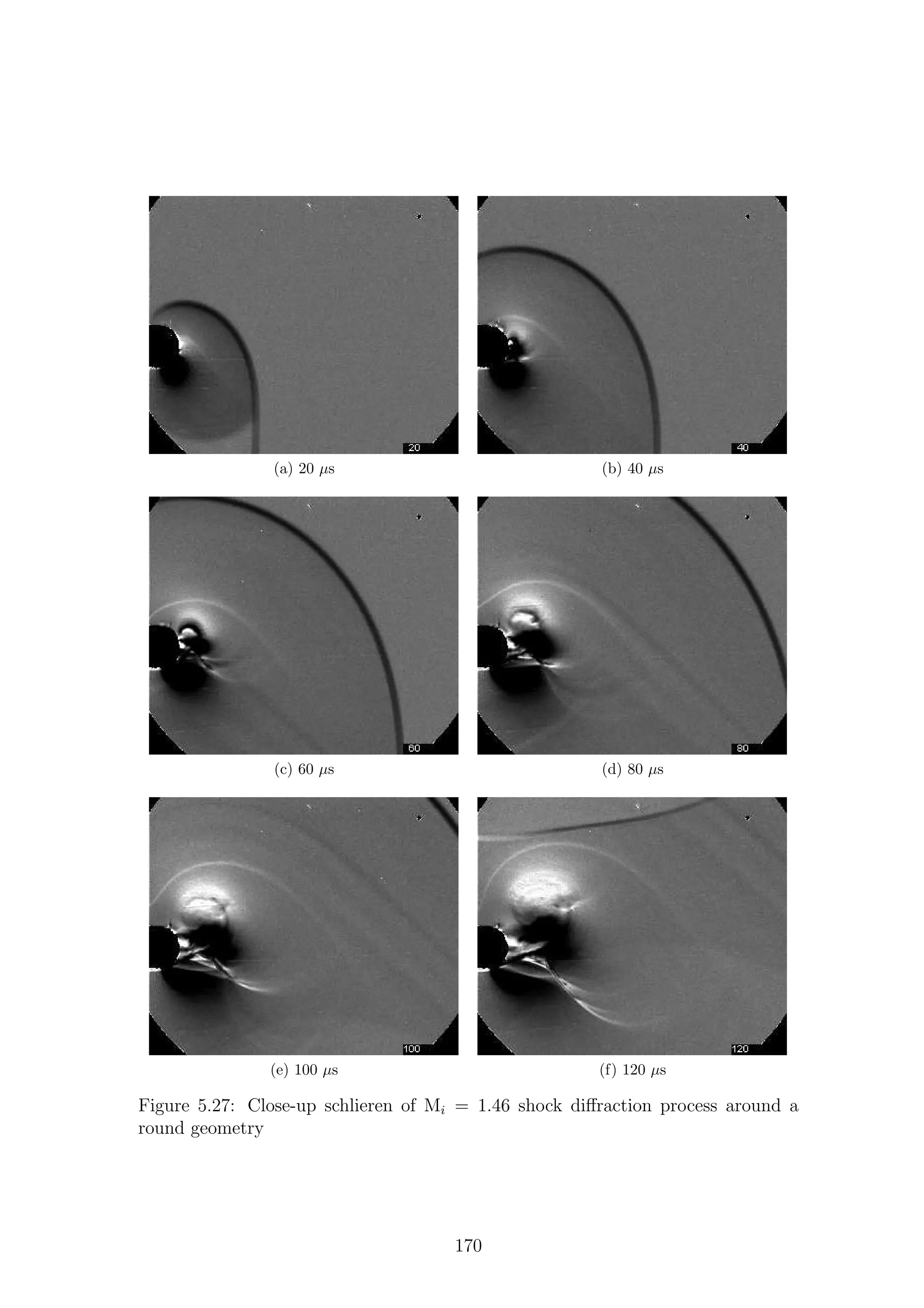
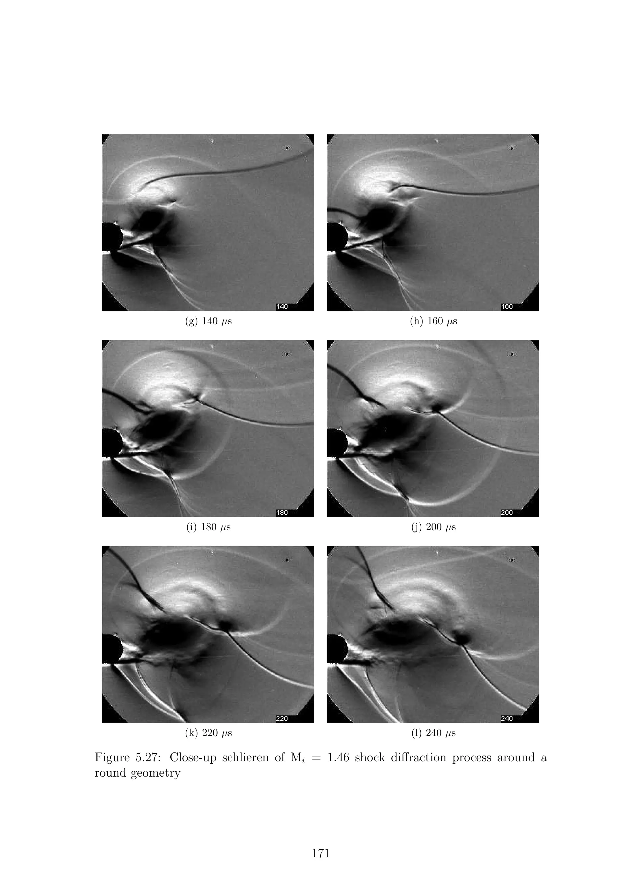
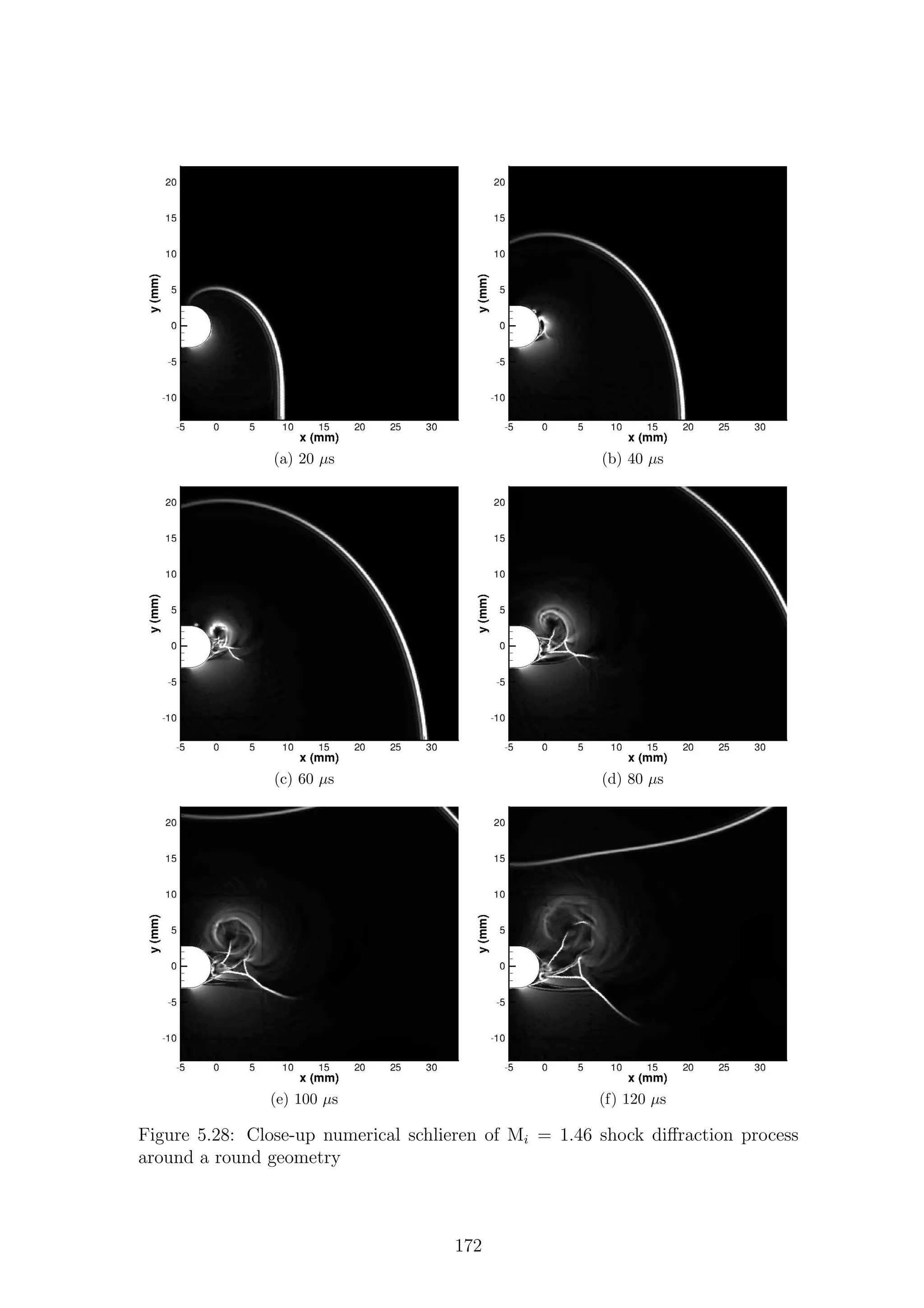
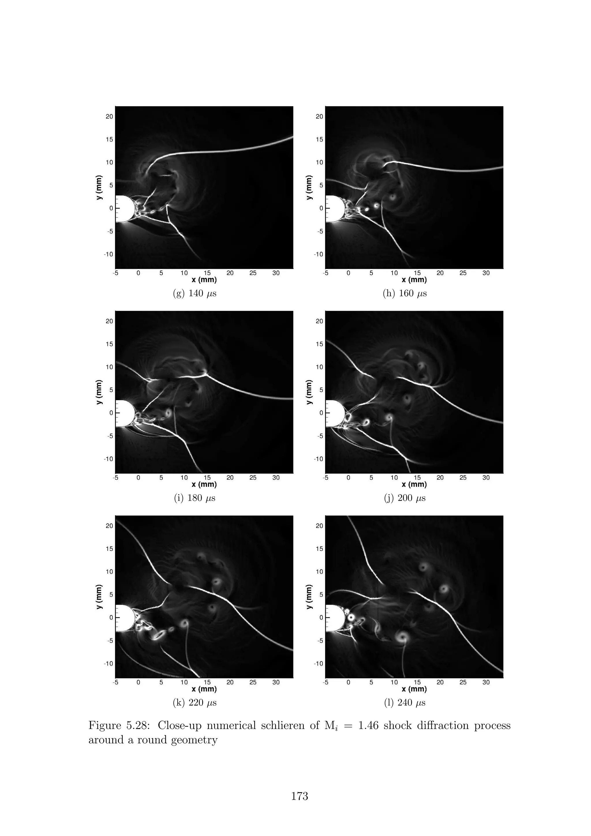
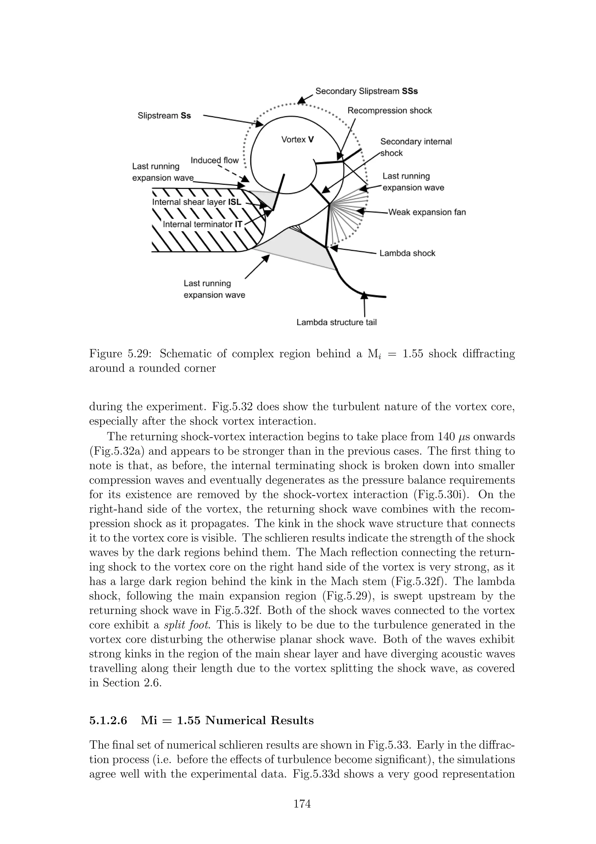
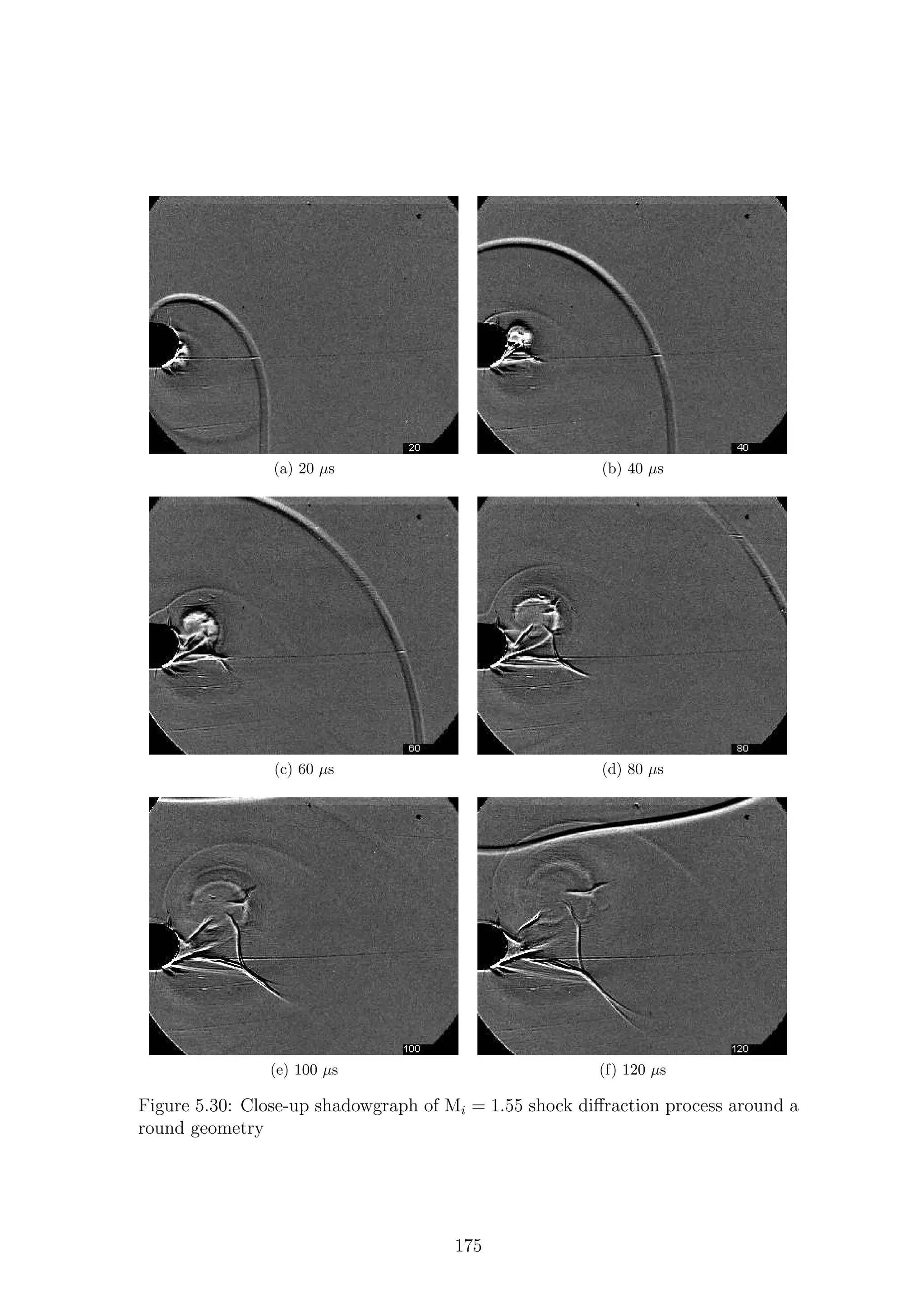
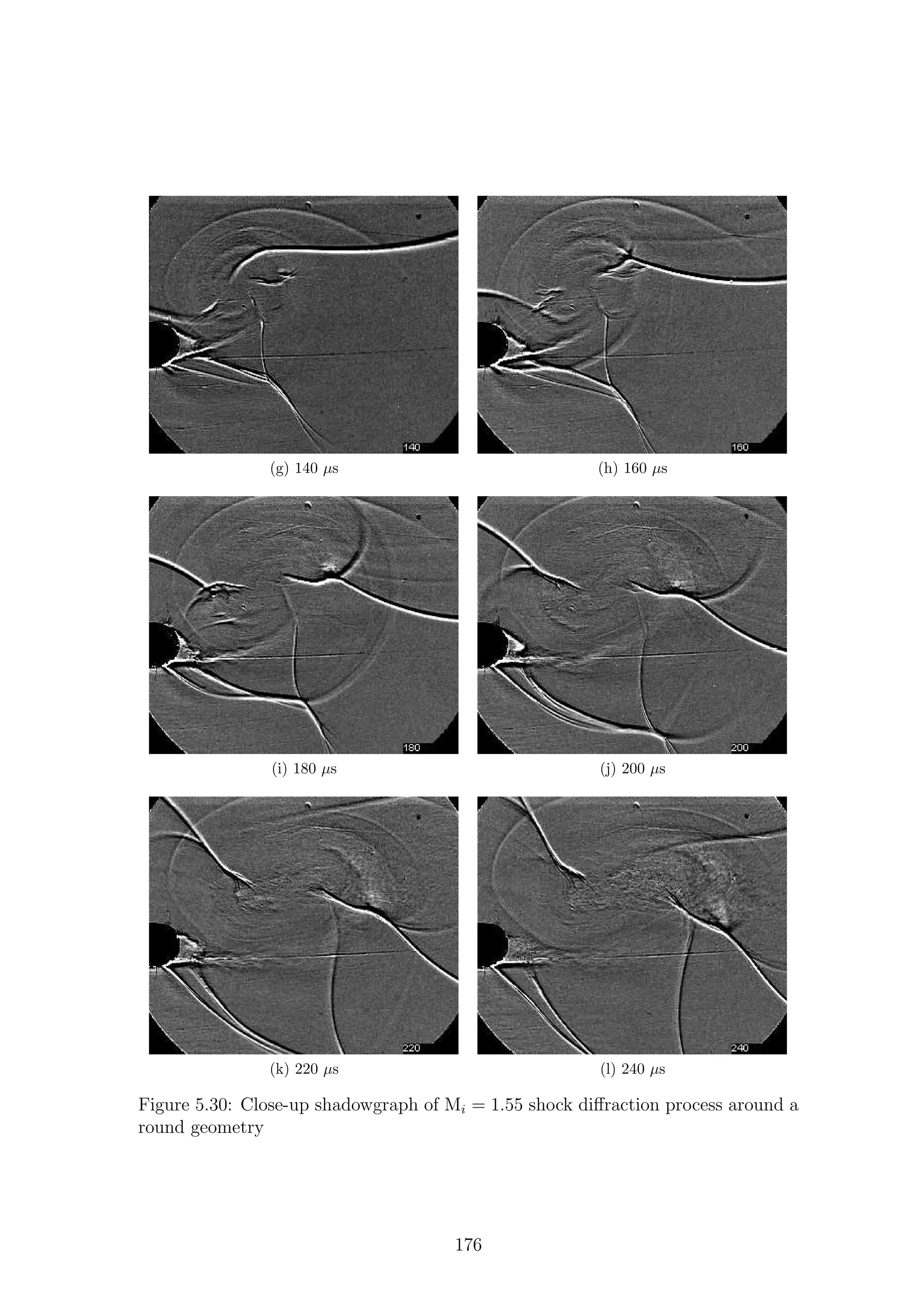
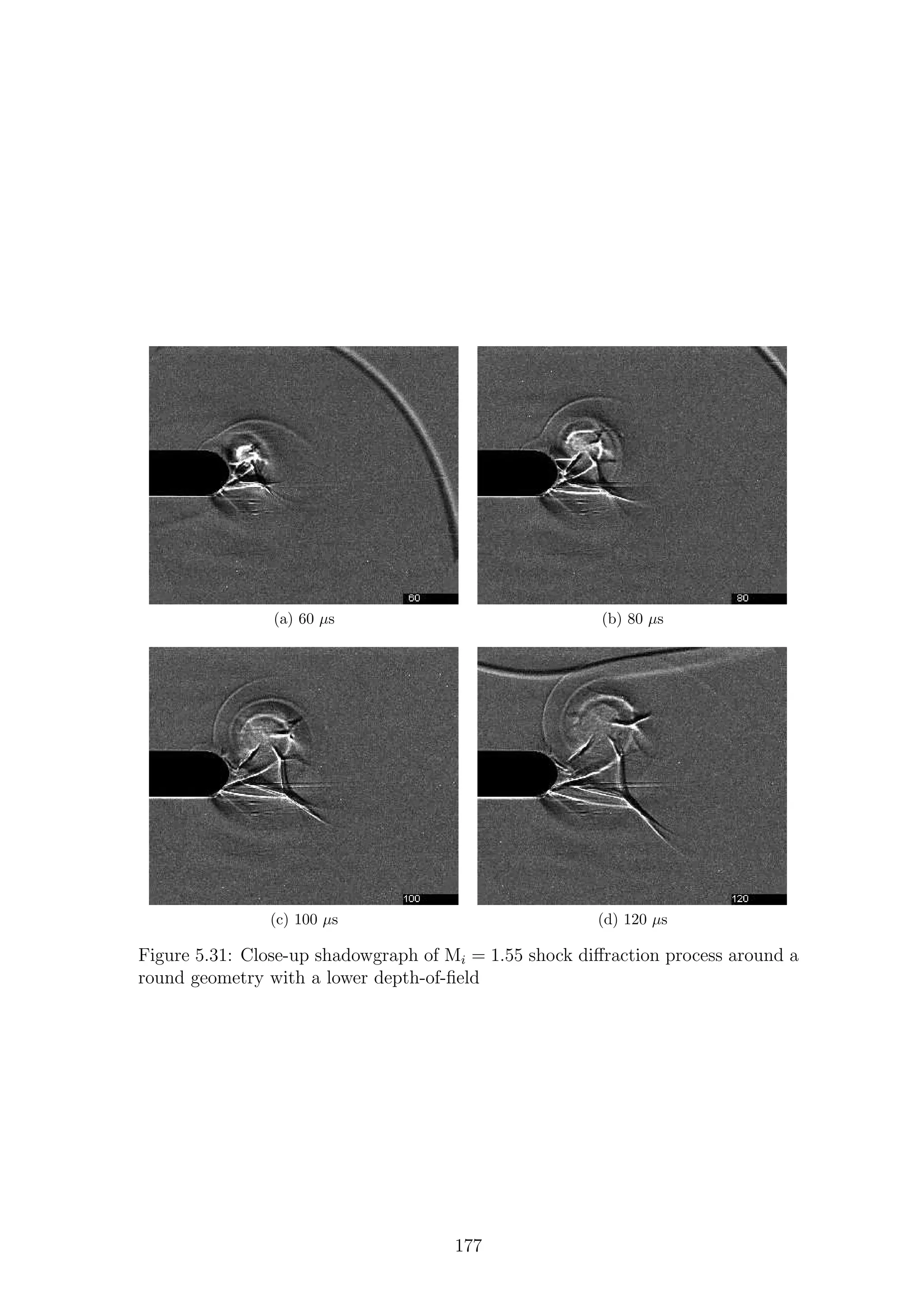
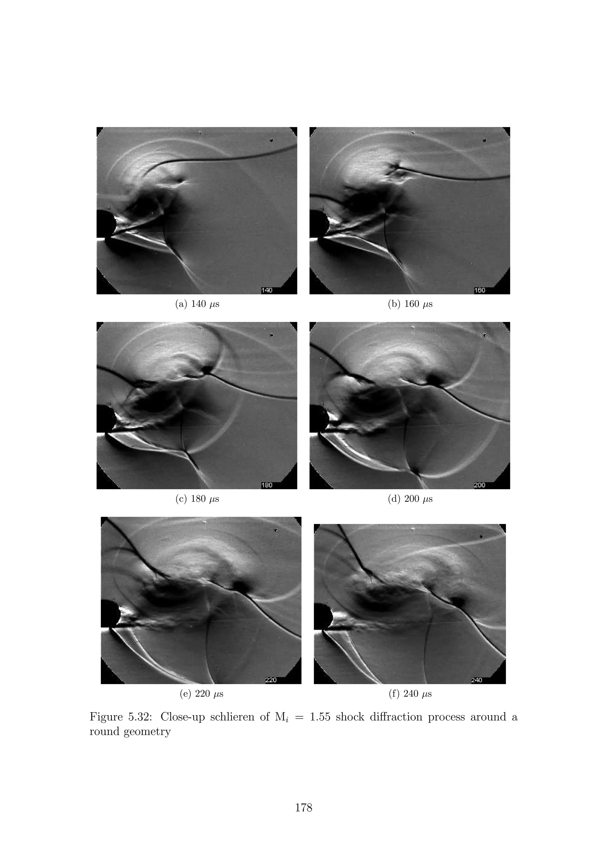
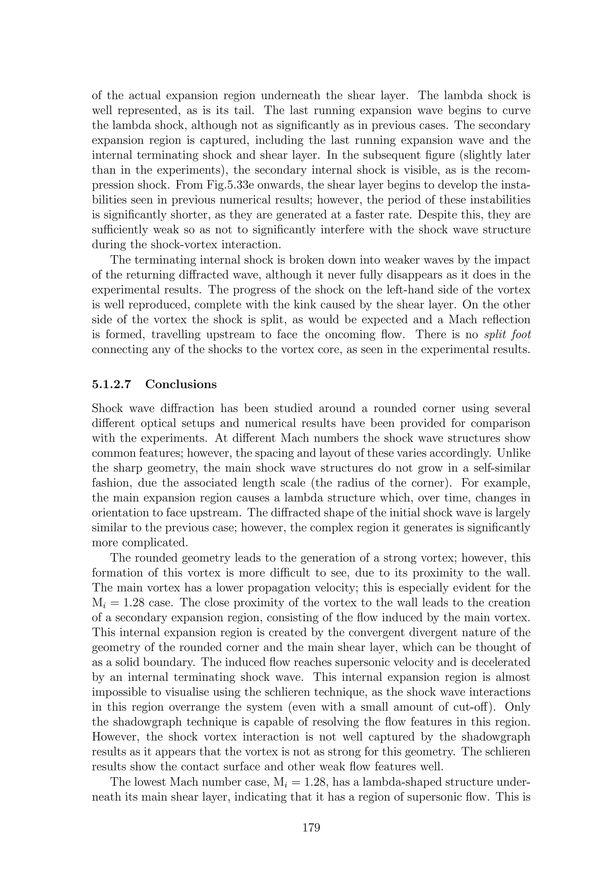

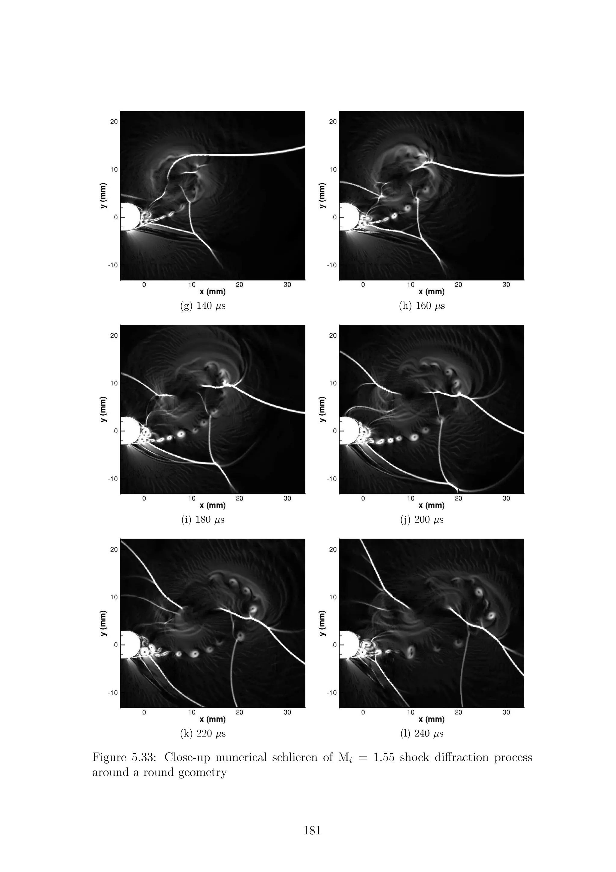
![in contrast with the theory of Sun & Takayama [36], which predicts that the critical
incident shock Mach number for a region of supersonic expansion is Mi = 1.35. The
expansion wave in this flow has a larger area to act over, given the distributed nature
of the geometry involved. This will be expanded upon further in Section 5.4.2.
The lambda structures indicate an incorrectly expanded region, followed by a
shock required to match the pressure condition imposed elsewhere in the flow field.
The Mi = 1.28 case showed a pair of these lambda structures; however, subsequent
Mach number cases showed a more complex, albeit single, wave pattern. Higher
Mach number cases exhibited a concave shear layer (unlike the Mi = 1.28 case),
allowing the already supersonic flow to expand more. This is especially evident at
Mi = 1.55. The internal terminating shock wave creates a jump in pressure which
causes a change of curvature of the main shear layer, leading to the creation of a
compression corner and the subsequent lambda shock.
The numerical simulations accurately predicted the boundary separation and
the movement of the separation point. The basic wave structures are captured,
including the internal expansion region. For this geometry, the shear layer is created
by a separated boundary layer which will be thicker than the one created by a sharp
corner, which can be thought of as inviscid separation. The presence of viscosity
plays an important role in the development of the flow around a rounded geometry
and, as such, it should be expected that a laminar model can only represent a
finite amount of flow development. Due to the high flow speeds involved, it will
not take long for the boundary layer to become turbulent and begin to invalidate
the assumptions of the laminar model used. This is especially a problem in the
Mi = 1.28 case, where the simulation begins to depart from the experiments after
160 µs, as the structures created are strong enough to interfere with the main wave
pattern development. Another manifestation of this problem can be found on the
main shear layer at higher Mach numbers. The numerical results develop instabilities
similar to those seen for the sharp geometry, which were not seen in the experimental
results. After a finite time, the real boundary layer will transition to turbulence,
providing a mechanism for energy transfer in the flow which is not reproduced in the
laminar simulations. This leads the laminar simulations to create sinks for energy
which cannot be transported elsewhere in the flow and is not lost through viscous
dissipation, i.e. vortices on the shear layer.
Thus far, it has been assumed that the flow in the shock tube is completely two-
dimensional. However, the shadowgraph results indicate that some of the waves
are no longer planar. This is caused by the turbulence in the boundary layer, as
turbulence is an inherently three-dimensional phenomenon. Although the flow is
no longer completely two-dimensional, the disturbances introduced do not appear
large enough to significantly affect the flow development. This means that the two-
dimensional simulations are still of use for comparison with the experimental results
in subsequent sections.
The shock vortex interaction is largely similar to the one presented for the sharp
geometry, with some minor differences. The waves T1 and RR′′
1 in Fig.5.18 propagate
more slowly around the vortex. This indicates that the oncoming flow is much faster
than for the sharp geometry. The lack of coherent structures propagating along the
shear layer means that the shock vortex interaction does not have the same diverging
acoustics created by the serially arranged K-H vortices found for the sharp case. The
strongest wave seen is the wave MR3 which is followed by a large change in image
182](https://image.slidesharecdn.com/4a6f74b5-6bbb-4ffd-b3f5-7486cdb057cd-150303082443-conversion-gate01/75/Mark-Quinn-Thesis-213-2048.jpg)

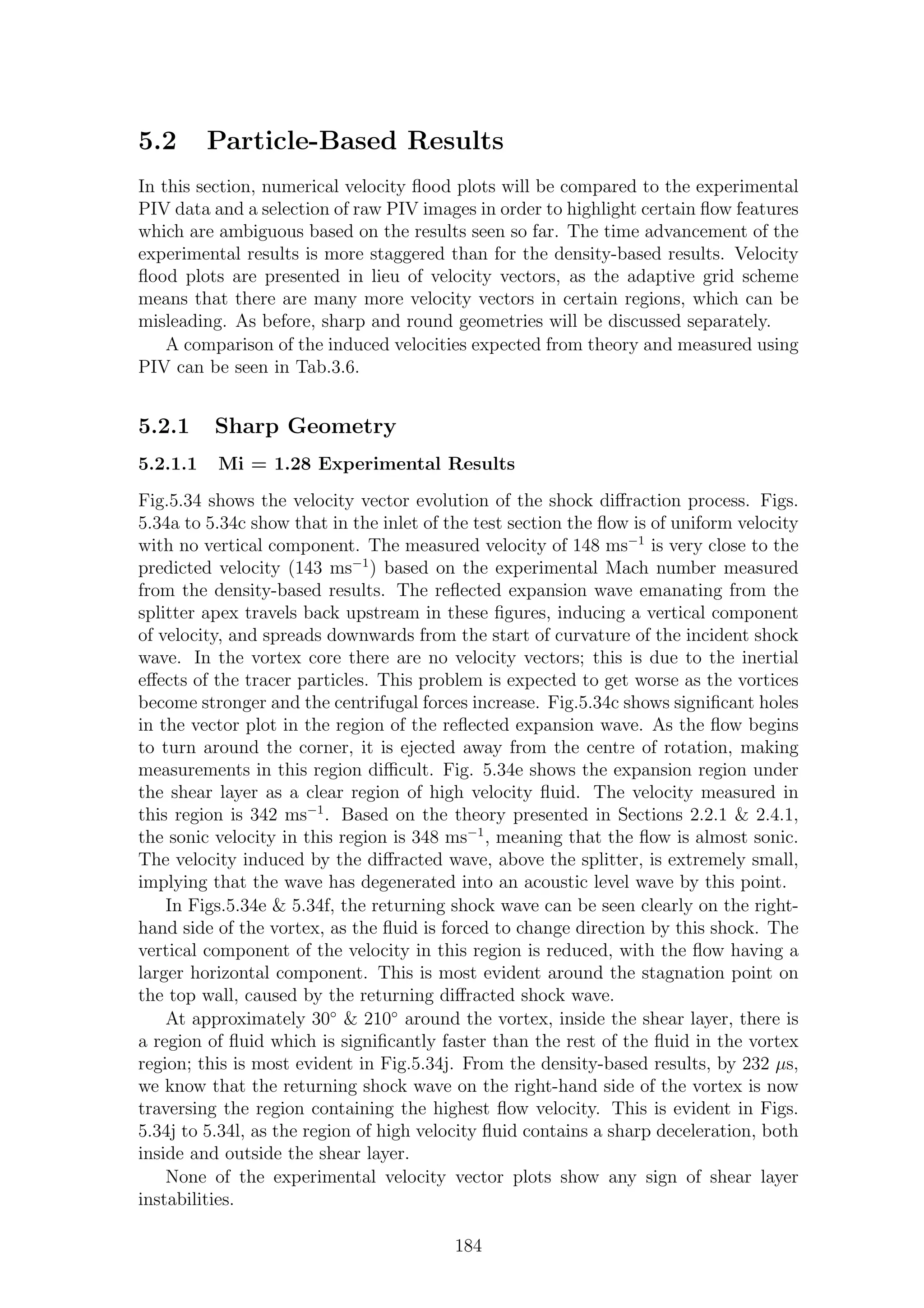
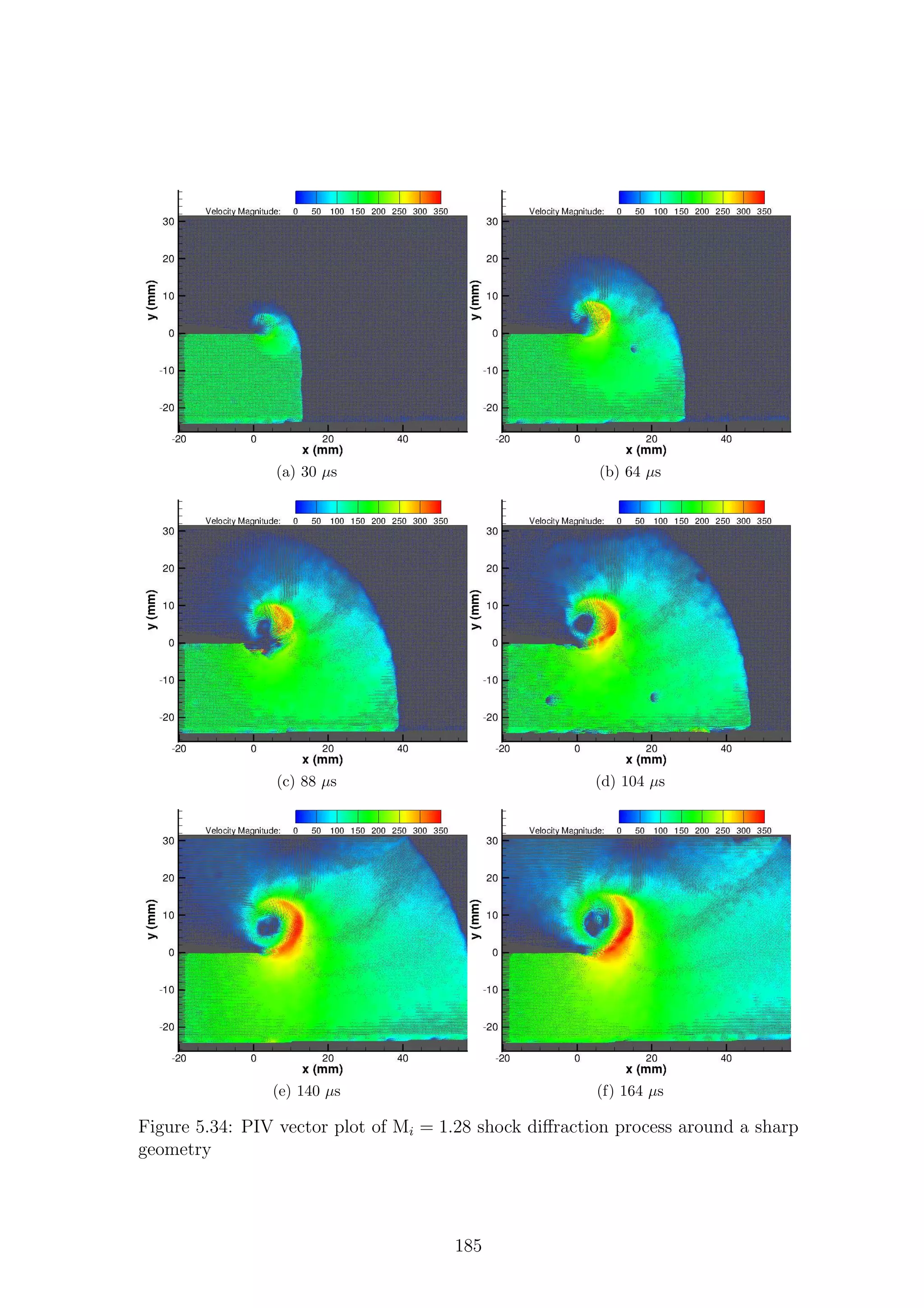
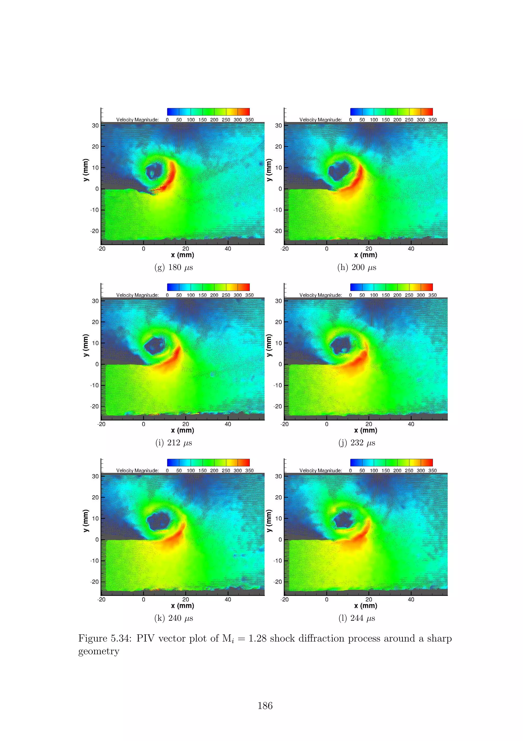
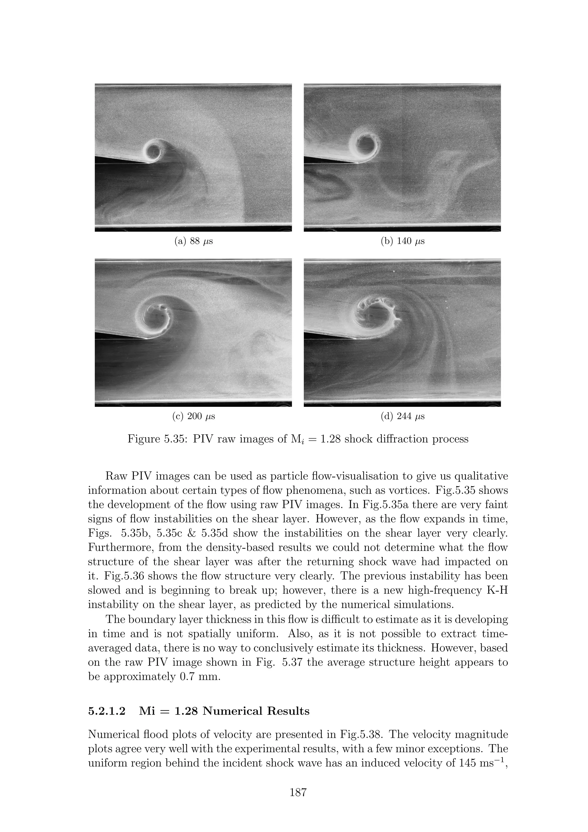
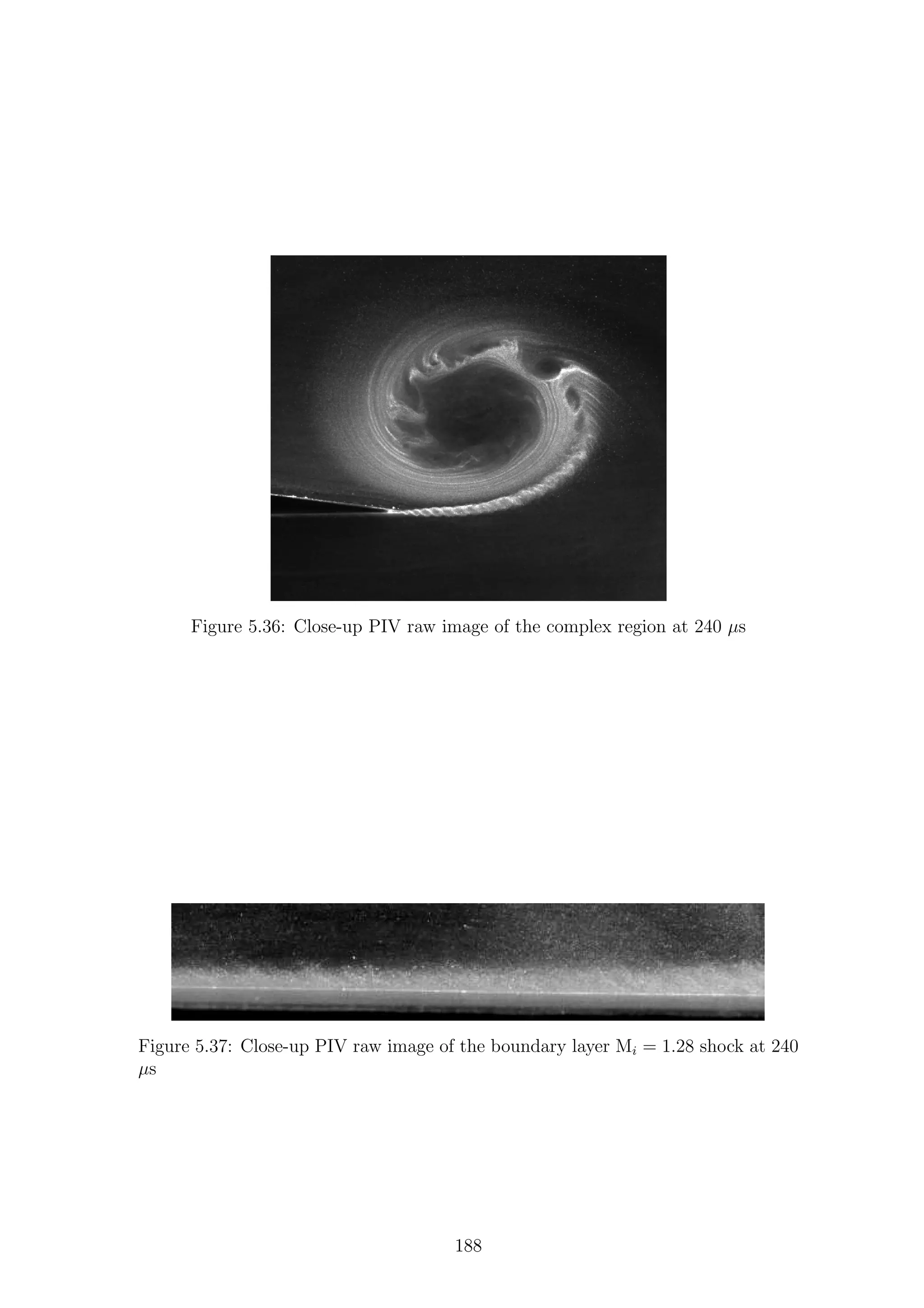
![which compares very well with the experimental and analytical values. The region of
high-velocity fluid has a slightly higher velocity in the simulations compared to the
experiments, with a maximum of 369 ms−1
, meaning that there are localised pockets
of supersonic flow. The maximum values are around the shear layer instabilities,
although they do not have as large an influence here as in subsequent tests. The
velocity just outside the shear layer reached 352 ms−1
. In the simulations it is
predicted to be slightly supersonic, which disagrees with the theory presented by
Sun & Takayama [36] which states that the critical Mach number is Mi = 1.346.
The stagnation point on the top surface of the test section can clearly be seen from
Fig.5.38e onwards. The region of high-velocity fluid on either side of the vortex
inside the shear layer can be seen in Fig.5.38j onwards. Figs.5.34l & 5.38l show the
decrease in velocity due to the returning diffracted shock wave as it passes through
the expansion region very clearly.
The numerical velocity flood plots show evidence of the shear layer instabilities
seen in the previous section.
5.2.1.3 Mi = 1.46 Experimental Results
Fig.5.39 shows the PIV vector plot of the Mi = 1.46 shock diffraction process. The
first thing to note in these images is the higher inlet velocity, 216 ms−1
, induced by
the stronger incident shock wave; this compares well with the experimental Mach
number prediction of 221 ms−1
. Velocity measurements in the vortex core remain
a problem, with little to no information available in those regions. Fig.5.39c shows
that the high velocity region is significantly larger in this case than in the previous
one, with a maximum velocity of 469 ms−1
. However, there is no sign of the lambda
shock structures seen in the density-based results. Although the expansion in this
region is stronger and therefore the velocity is higher, the lambda waves are not
strong enough to significantly change the velocity. The lambda structures are also
small enough that they are on the limit of what the PIV particles can be expected
to resolve given their relaxation time (Section 3.2.3) and could be smoothed out
by particle intertia. As in the previous case, the velocity induced by the diffracted
wave, above the splitter, is extremely small.
The stagnation region, seen as early as 104 µs, on the top surface of the test
section is larger in this test, indicating that the strength of the returning shock
wave is greater than before. The returning wave is again more visible to the right
of the vortex, due to the larger changes in flow direction in this region (Figs. 5.39f
to 5.39h).
Fig.5.39g onwards show regions of high-velocity fluid on the top side and bottom
side of the vortex. These are especially noticeable from Fig.5.39i onwards, where the
double shock structure to the left of the vortex (see Fig.5.8j to 5.8l) seems to end
the region of high-speed flow. Below the vortex but above the shear layer, the flow
is accelerated to speeds approaching those seen below the shear layer (Figs.5.39j to
5.39l). The regions both inside and outside the shear layer are decelerated by the
returning shock wave, as seen in Fig.5.8k; however, the region inside is decelerated
further upstream, as the shock has been able to propagate faster in this region due
to the slower oncoming flow.
After the returning shock has impacted on the shear layer, the expansion region
is drawn further and further towards the bottom of the test section, inducing a high
189](https://image.slidesharecdn.com/4a6f74b5-6bbb-4ffd-b3f5-7486cdb057cd-150303082443-conversion-gate01/75/Mark-Quinn-Thesis-220-2048.jpg)
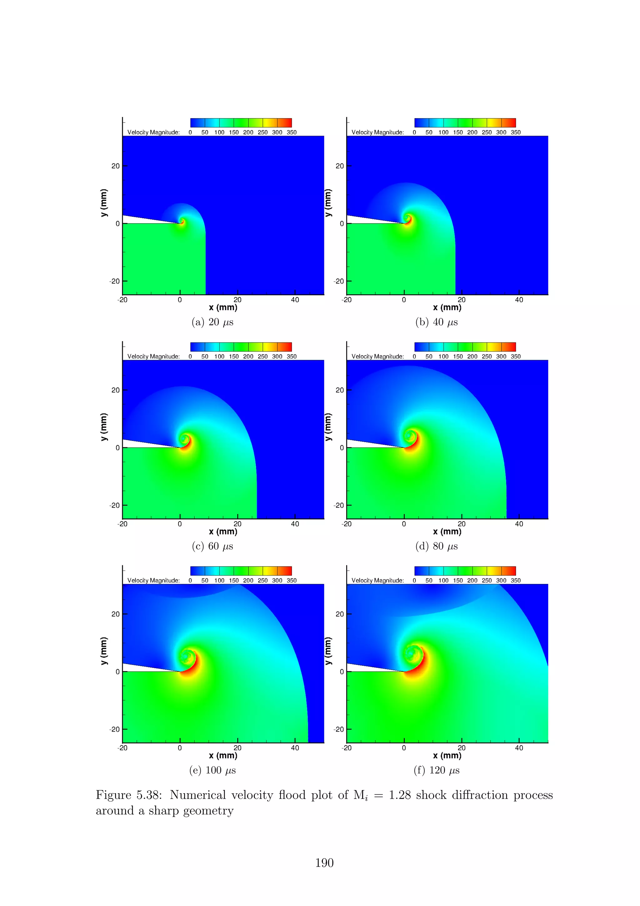
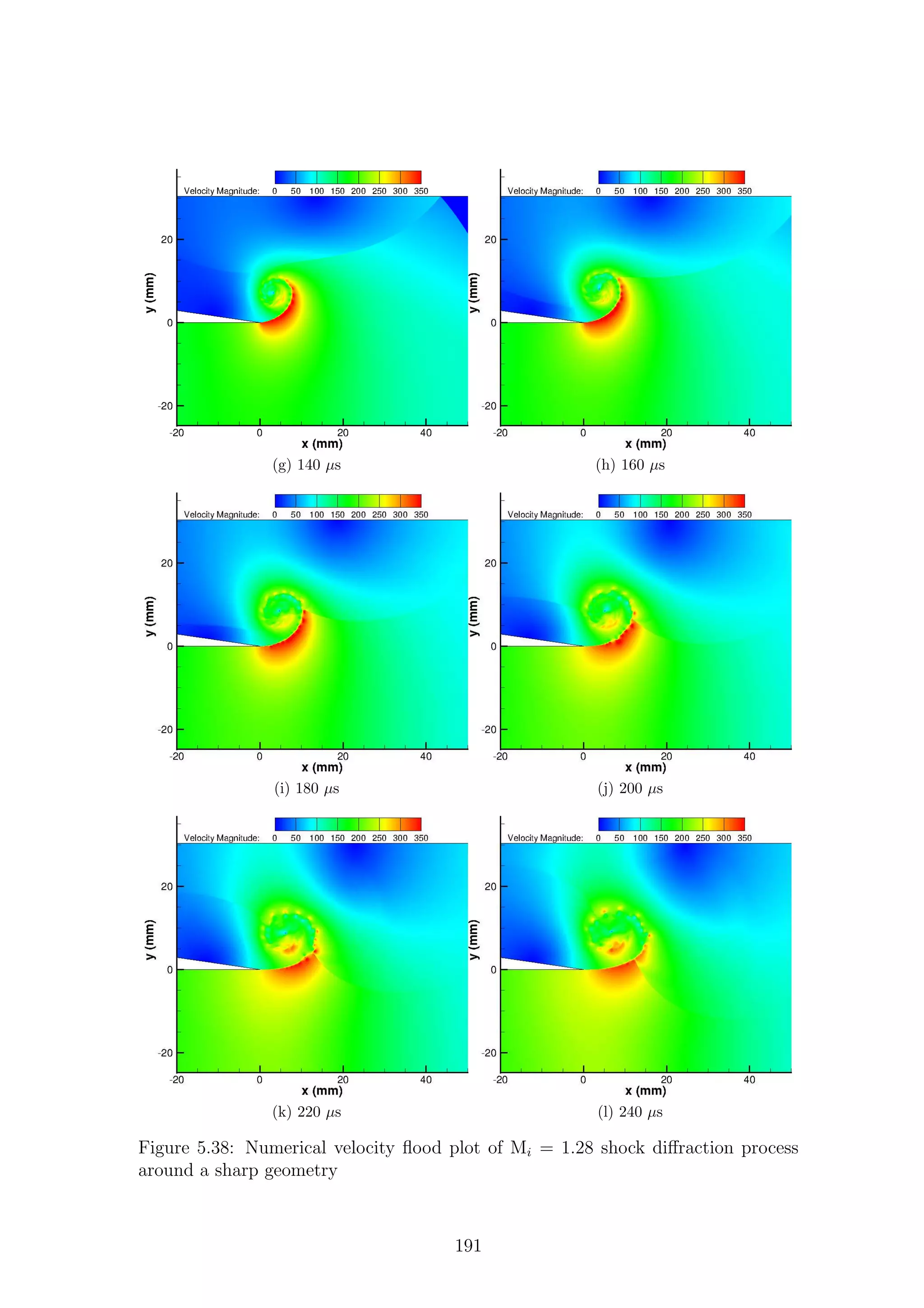
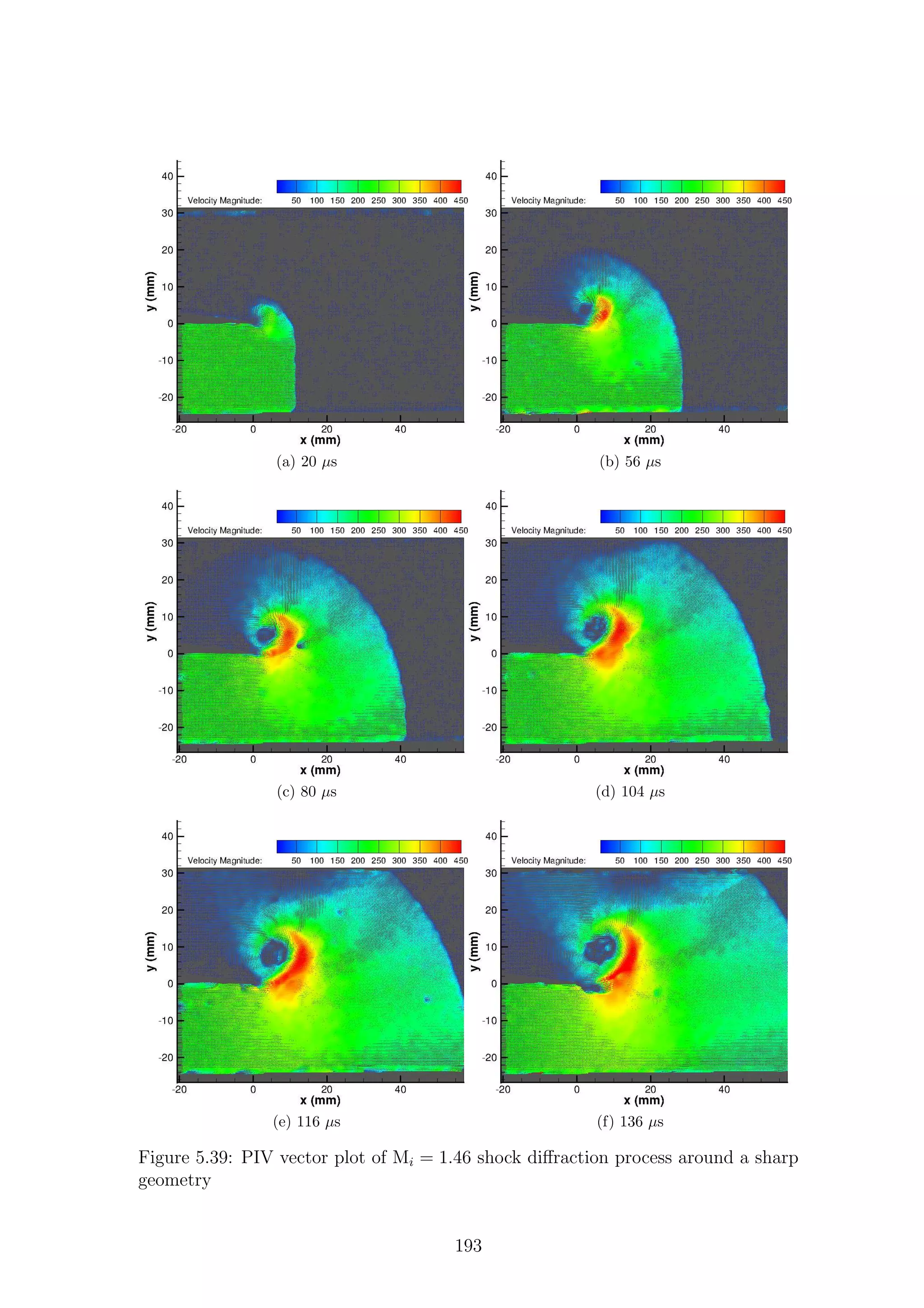
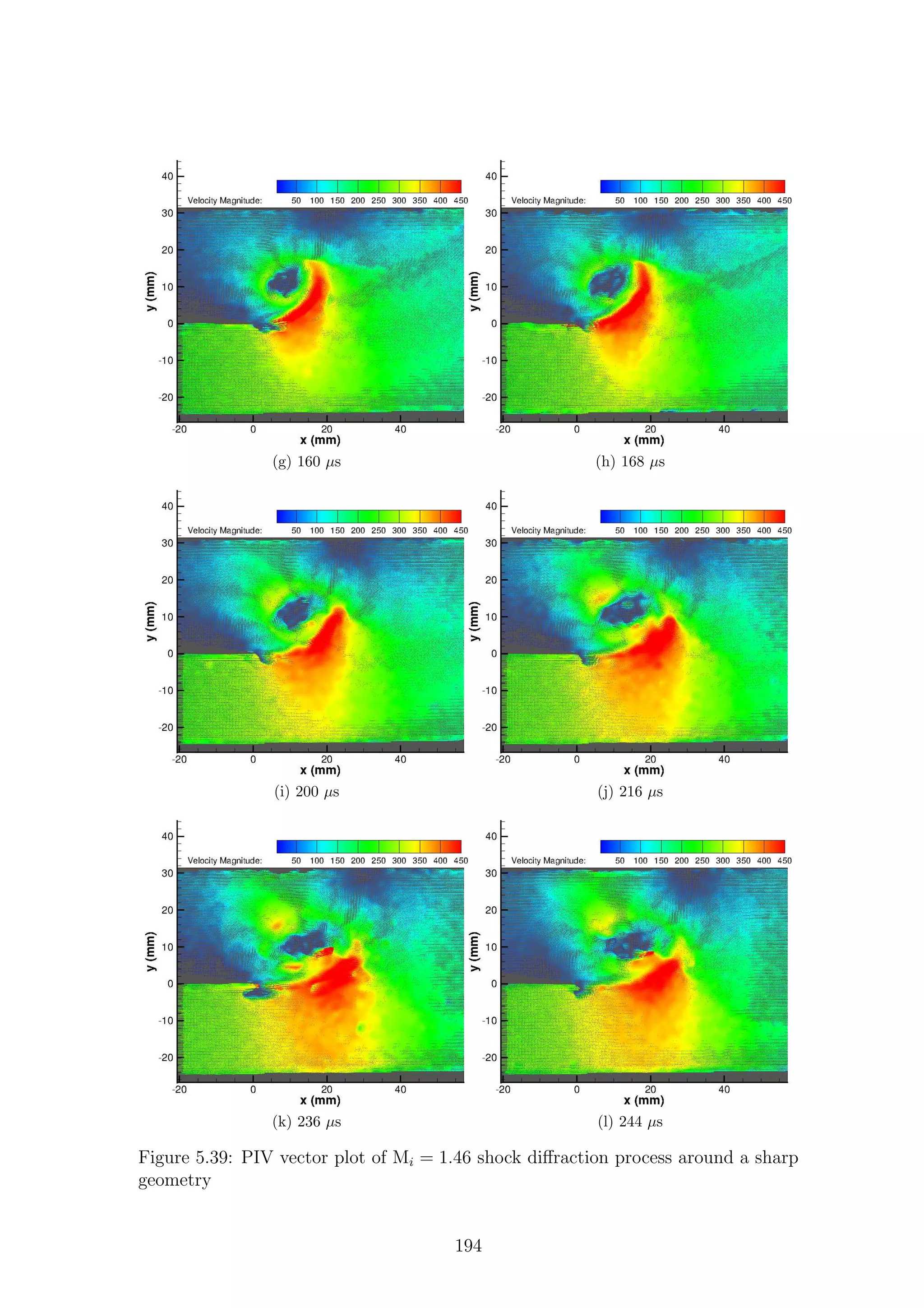
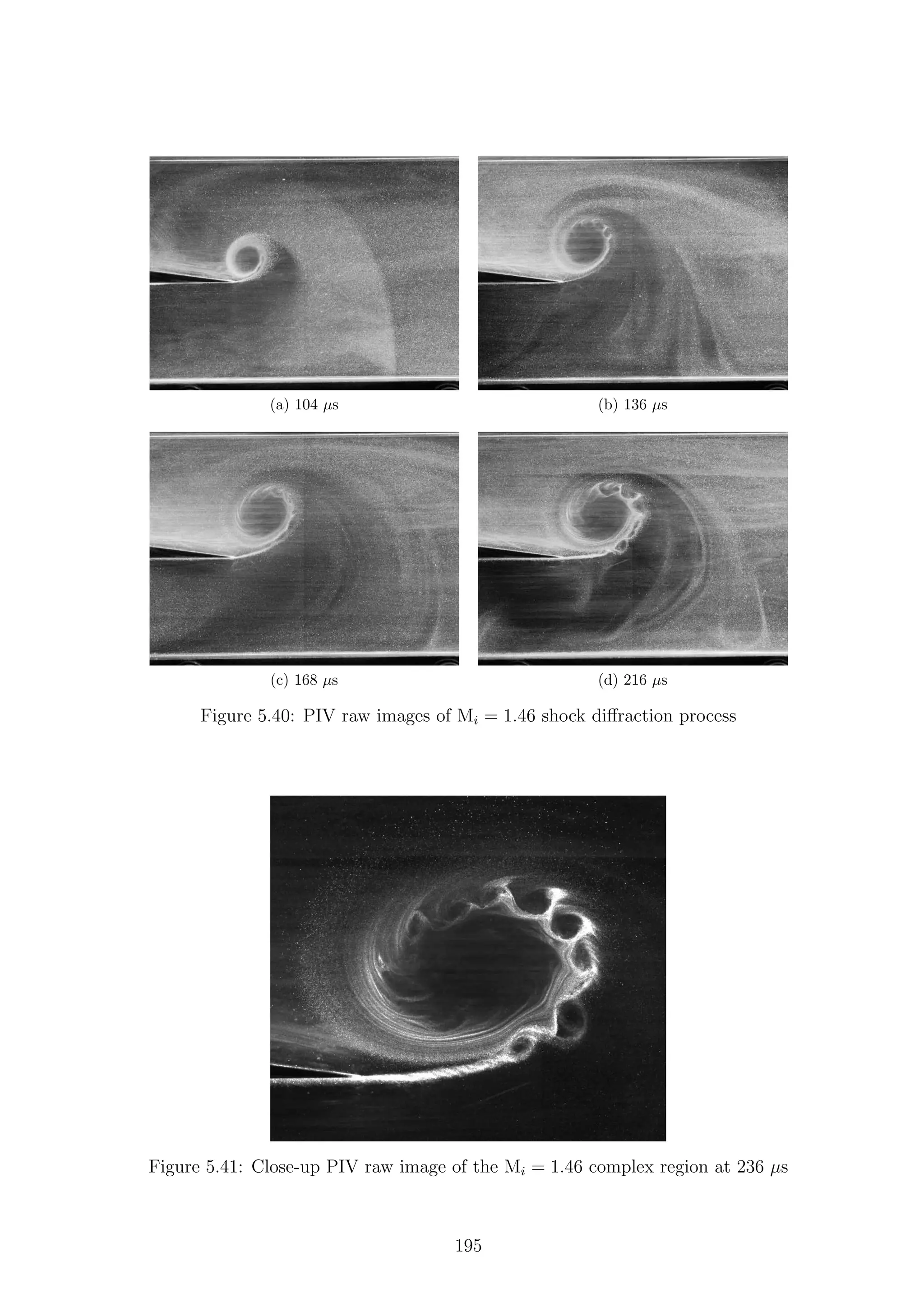
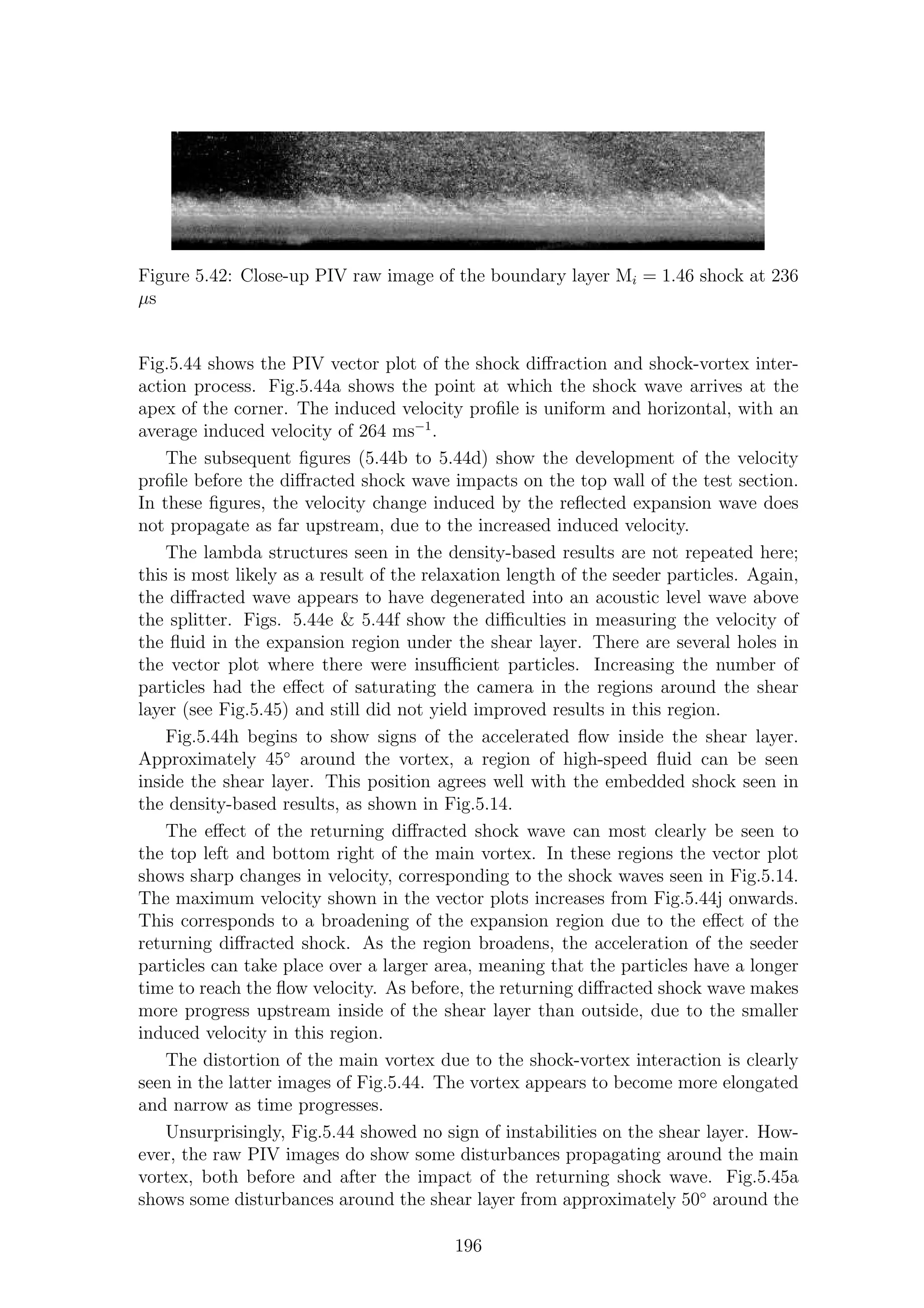

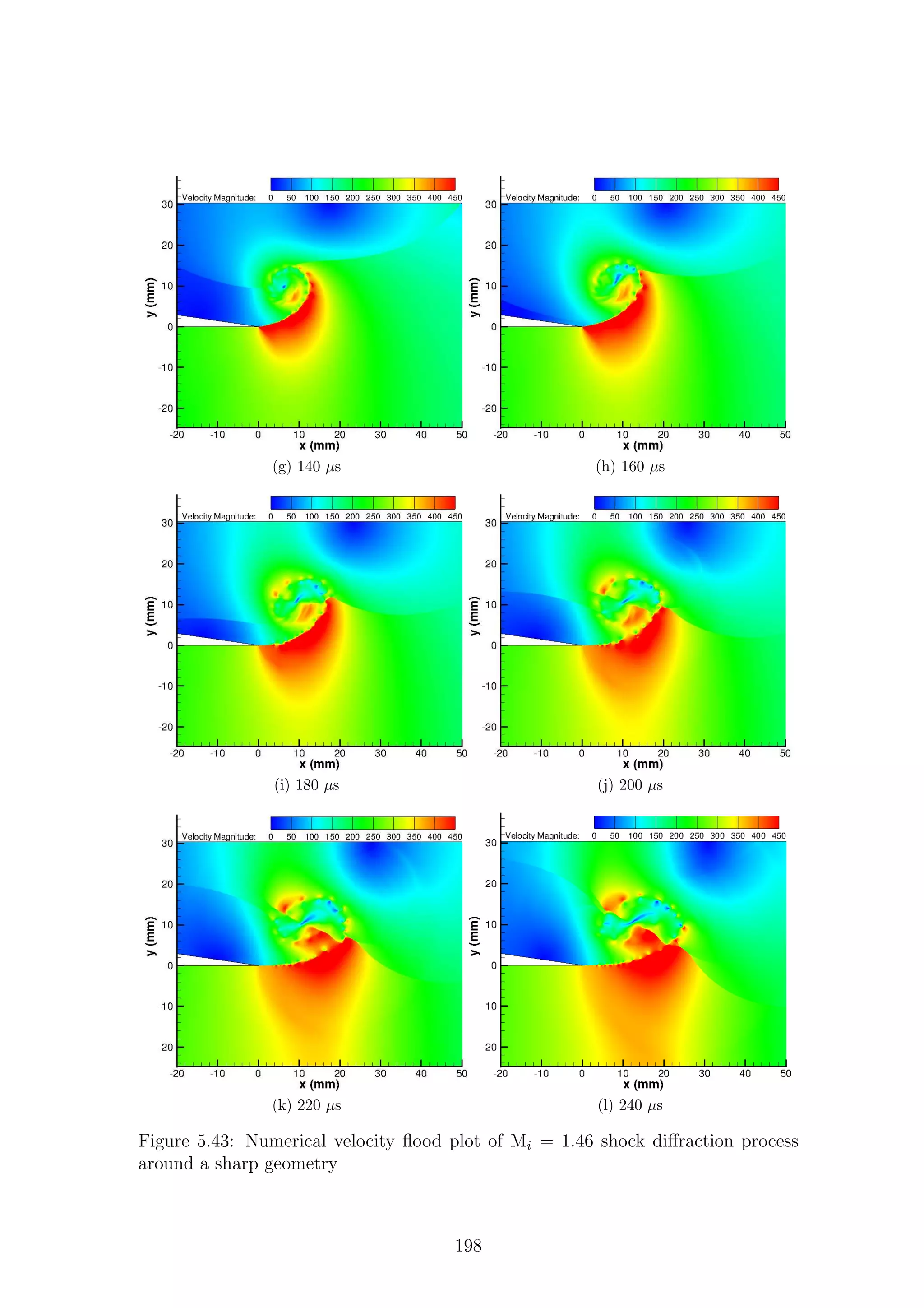
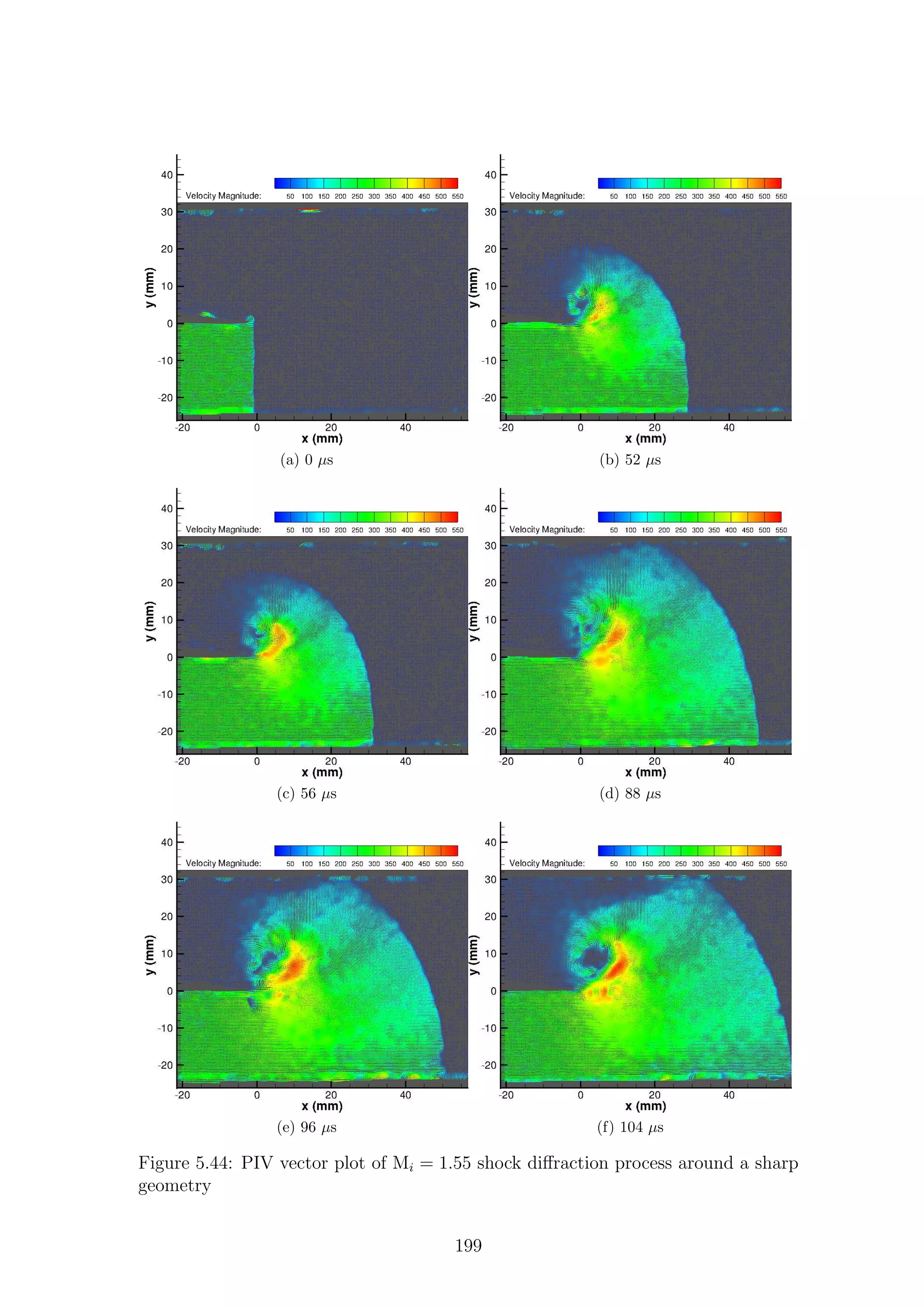
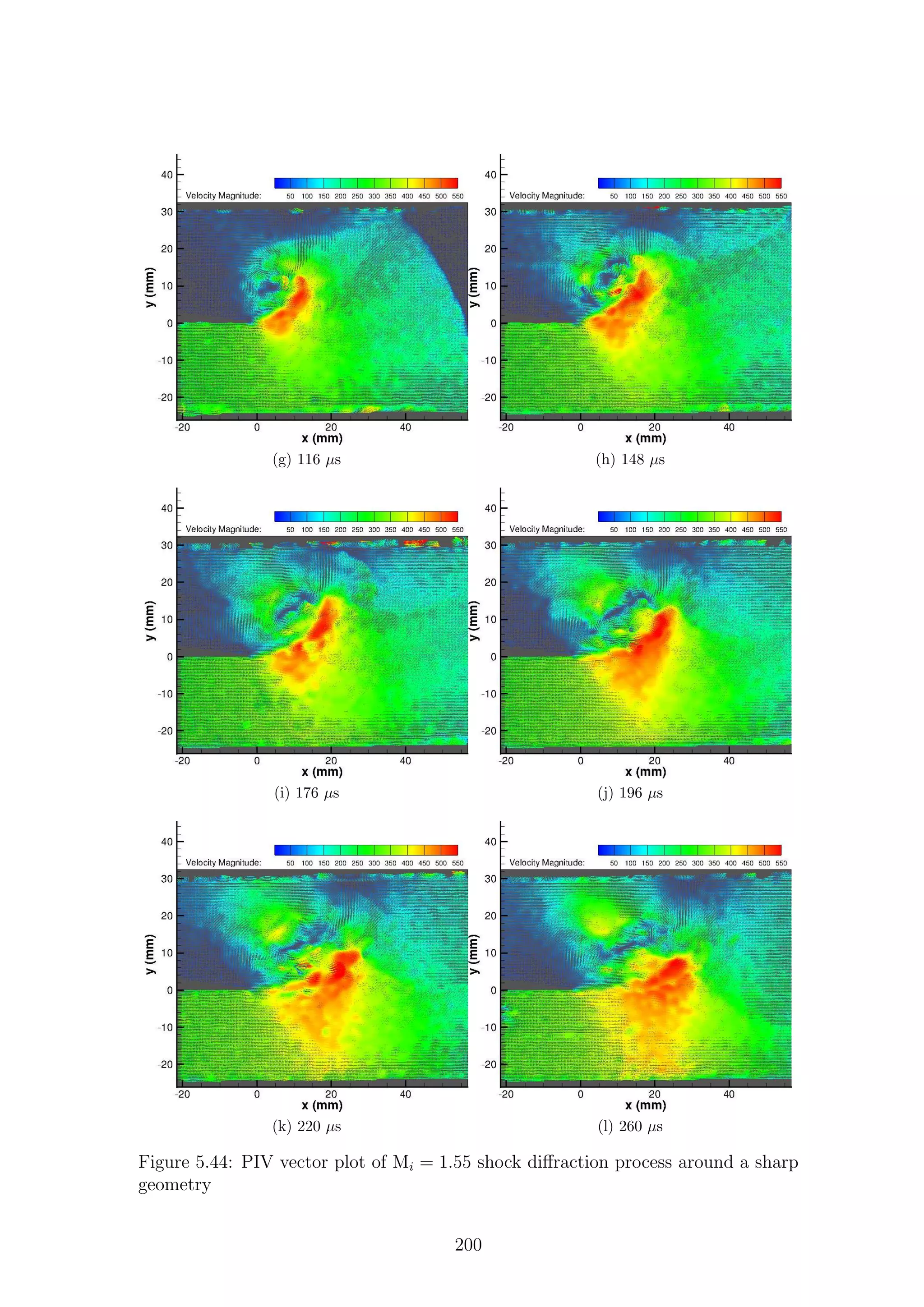
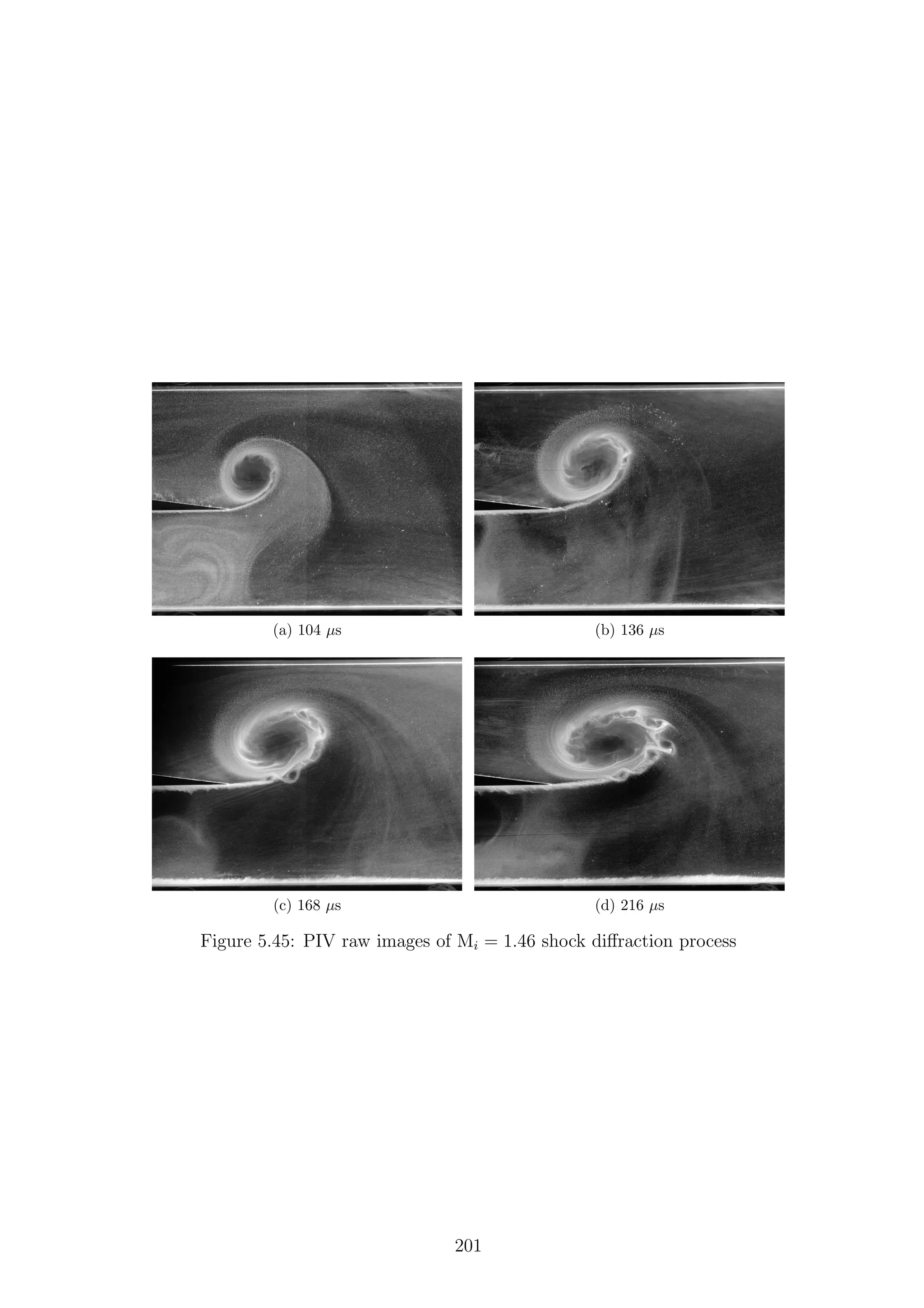
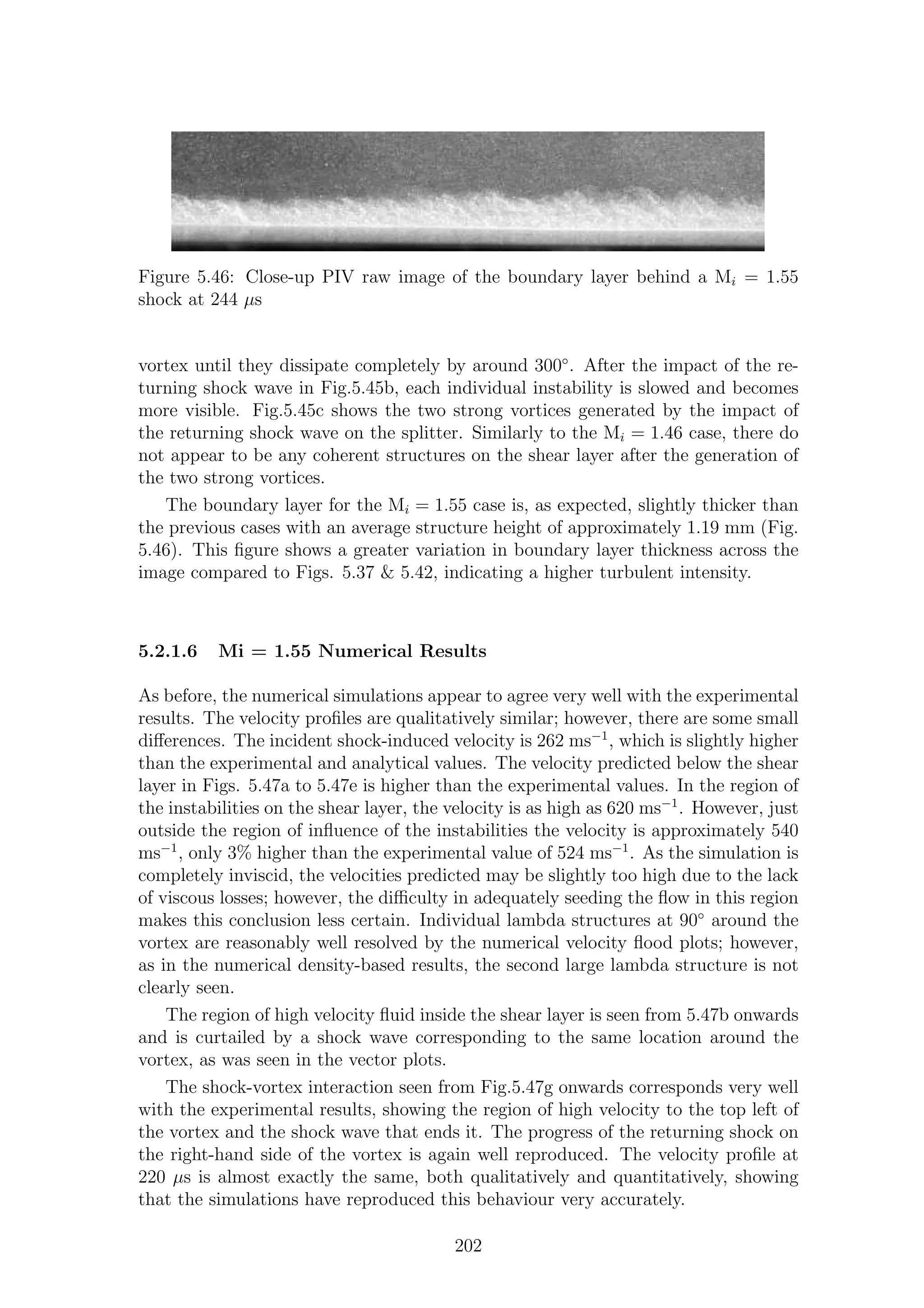
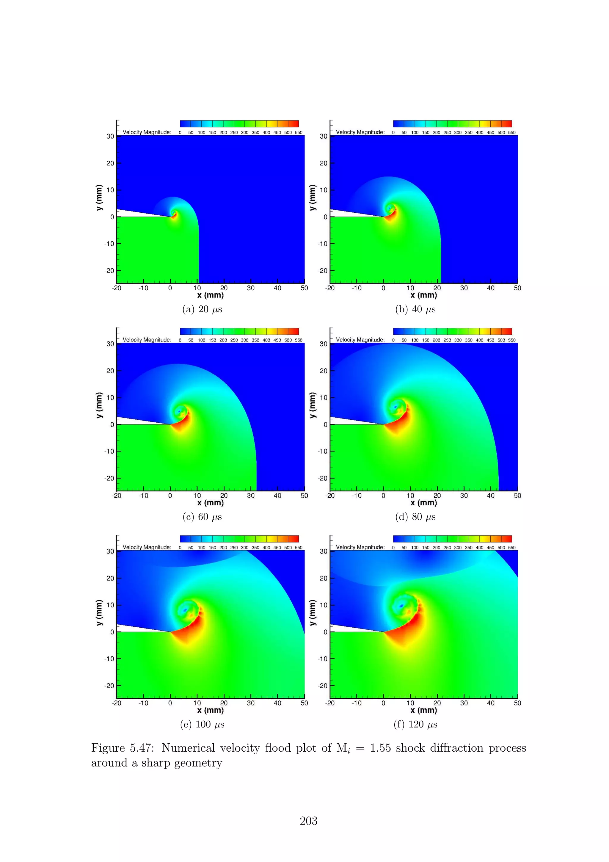
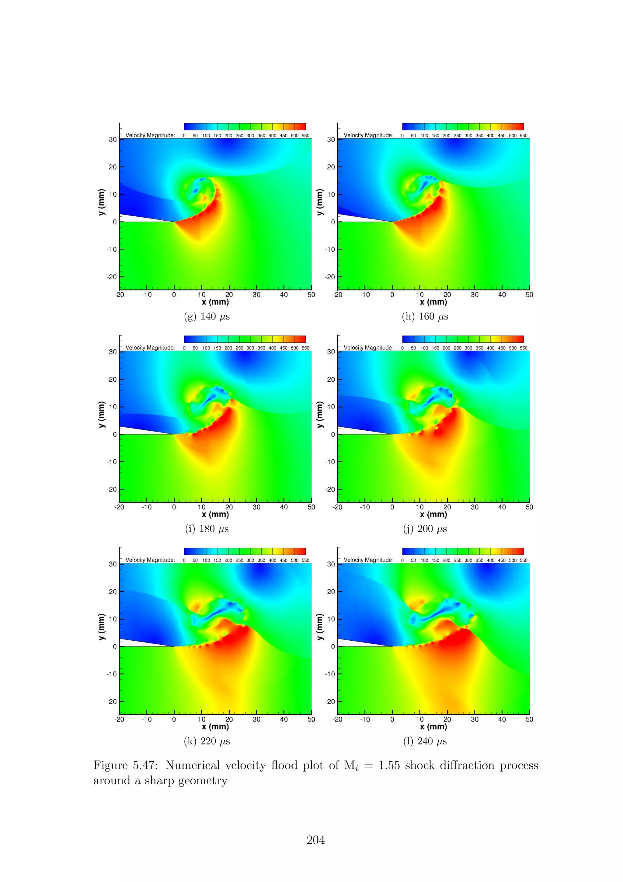

![5.2.2 Round Geometry
5.2.2.1 Mi = 1.28 Experimental Results
Fig.5.48 shows the time evolution of the flow around a rounded corner. As with
the sharp geometry, there is no vertical component of velocity until the influence
of the reflected expansion wave is felt by the flow. The inlet velocity is 141 ms−1
,
which compares very well with the predicted velocity of 143 ms−1
. The shock front
is well resolved and shows the expected curvature as it diffracts around the corner.
Figs. 5.48a & 5.48b show no signs of flow separation around the corner, as there
are no holes in the vector plot and no recirculation in the flow. However, by 64 µs
(Fig.5.48c), there are signs of recirculation and some noticeable gaps in the data due
to non-uniform seeding. The velocity in the complex region is higher than in the
uniform inlet region, indicating the strength of the main vortex. The lack of uniform
seeding, especially inside the vortex, makes quantitative interpretation of the PIV
results in this area very difficult, as we know from the schlieren images that the
main vortex remains in close proximity to the wall for a significant amount of time.
There are regions of very high velocity fluid below the shear layer corresponding to
the expansion wave in this region; however, we know from the density-based results
that this structure is not very large, a finding repeated from the PIV results, as this
region is relatively small.
As the wave pattern expands in time, a stagnation point moves along the top
surface of the splitter in the corresponding location to the contact surface seen in the
density-based results. This observation indicates that the conclusion by Skews [32]
that the contact surface is a good indication of fluid motion is justified. Figs.5.48e &
5.48f show the diffracted shock wave reflecting off the top surface of the test section
and propagating downwards towards the complex region. By Fig.5.48h the vortex
has grown in size and strength to begin to eject particles from its core, leaving holes
in the vector plot indicating its centre. In this figure we can see that there is a
region of high-speed fluid between the vortex core and the rounded corner of the
splitter. This region of high-speed fluid corresponds to the location of the internal
expansion region discussed in Section 5.1.2. The slug of high-speed fluid persists in
all of the subsequent PIV vector plots and is terminated at the same location as the
internal terminating shock seen in Figs.5.19 & 5.20. Fig.5.48l shows a region of very
high-velocity fluid just below the vortex core. This high-velocity fluid corresponds
to the location of the strongest shock seen in the density-based results, MR3, as
discussed in Sections 5.1.1.7 & 5.1.2.7.
With the exception of the wave MR3, the shock-vortex interaction does not
appear to have significantly affected the flow, apart from transforming the vortex
into a more circular shape as there are no more strong discontinuities.
Throughout the development seen in Fig.5.48, there is no information available
about the structure of the shear layer(s) and the region immediately adjacent to the
splitter edge. The early raw PIV images show no distinct shear layer (Fig.5.49a).
At later times, after the shock-vortex interaction, the shear layer is more visible
(Fig.5.49b), although there does not appears to be any coherent structures present,
just random structures with no discernible pattern. Fig.5.49a shows the contact
surface and its impact point on the splitter clearly, along with the kink seen in
the schlieren images, indicating that the flow is being drawn into the vortex in
207](https://image.slidesharecdn.com/4a6f74b5-6bbb-4ffd-b3f5-7486cdb057cd-150303082443-conversion-gate01/75/Mark-Quinn-Thesis-238-2048.jpg)
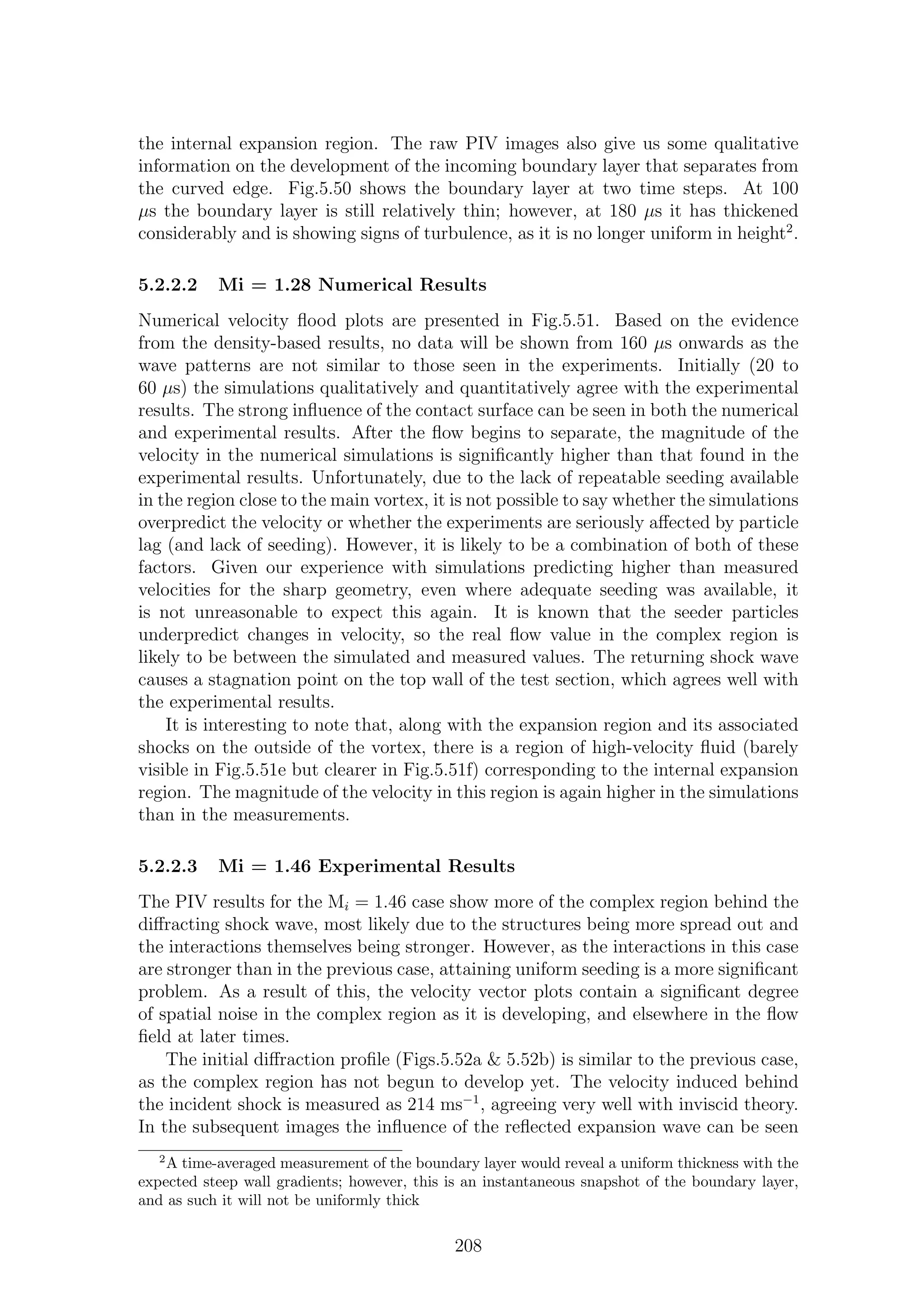
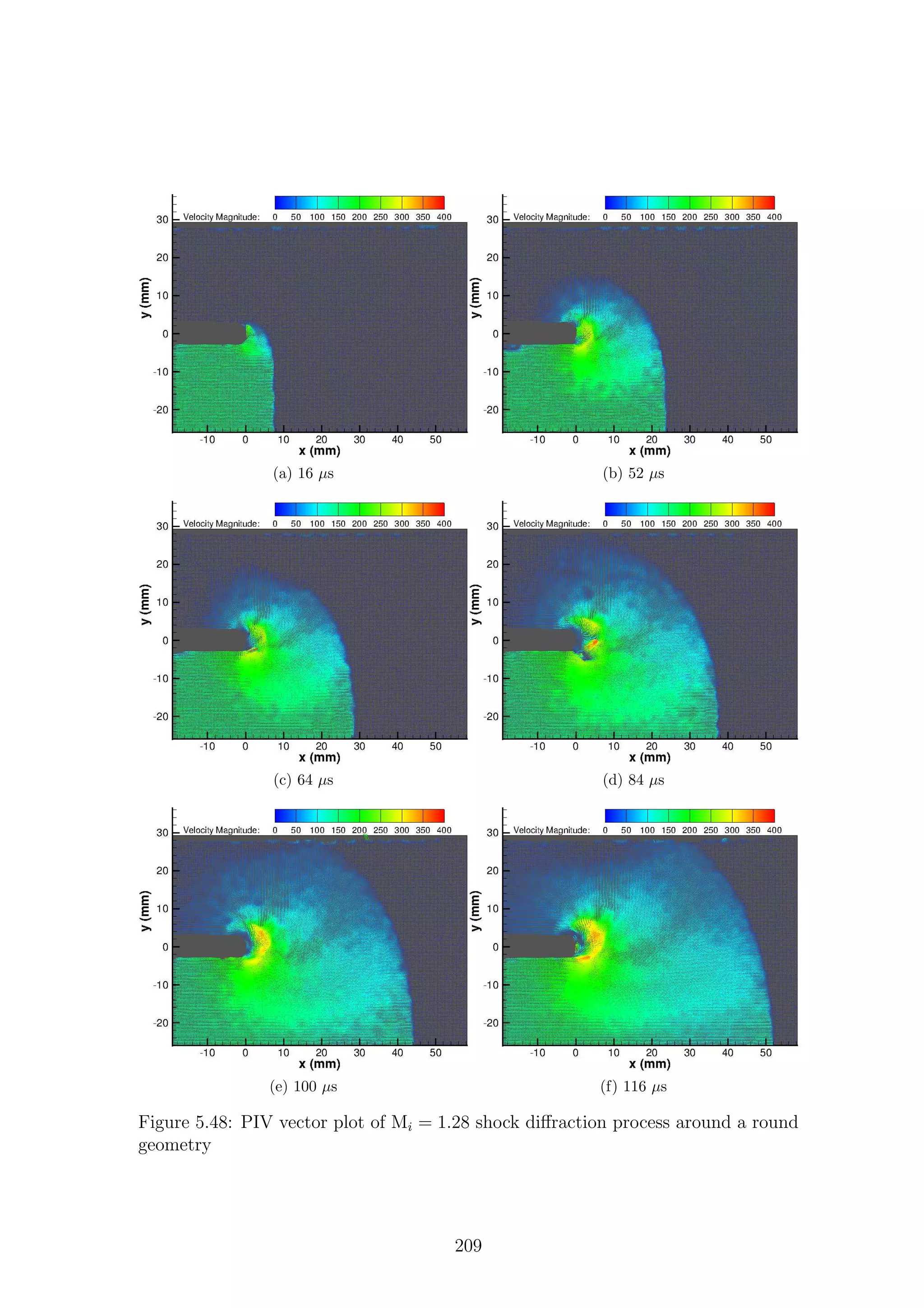
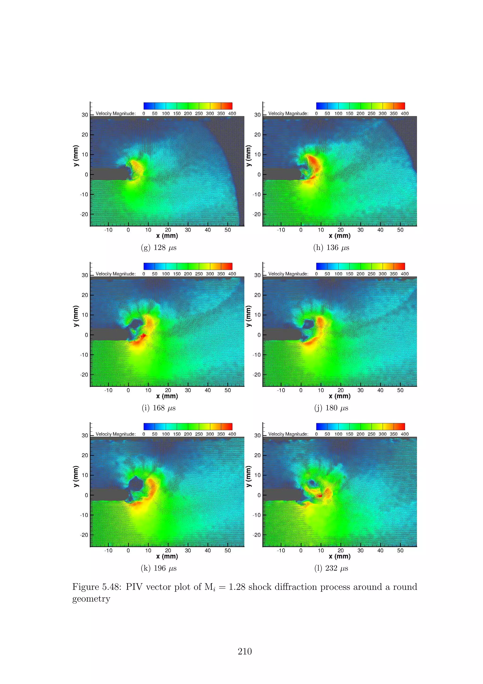
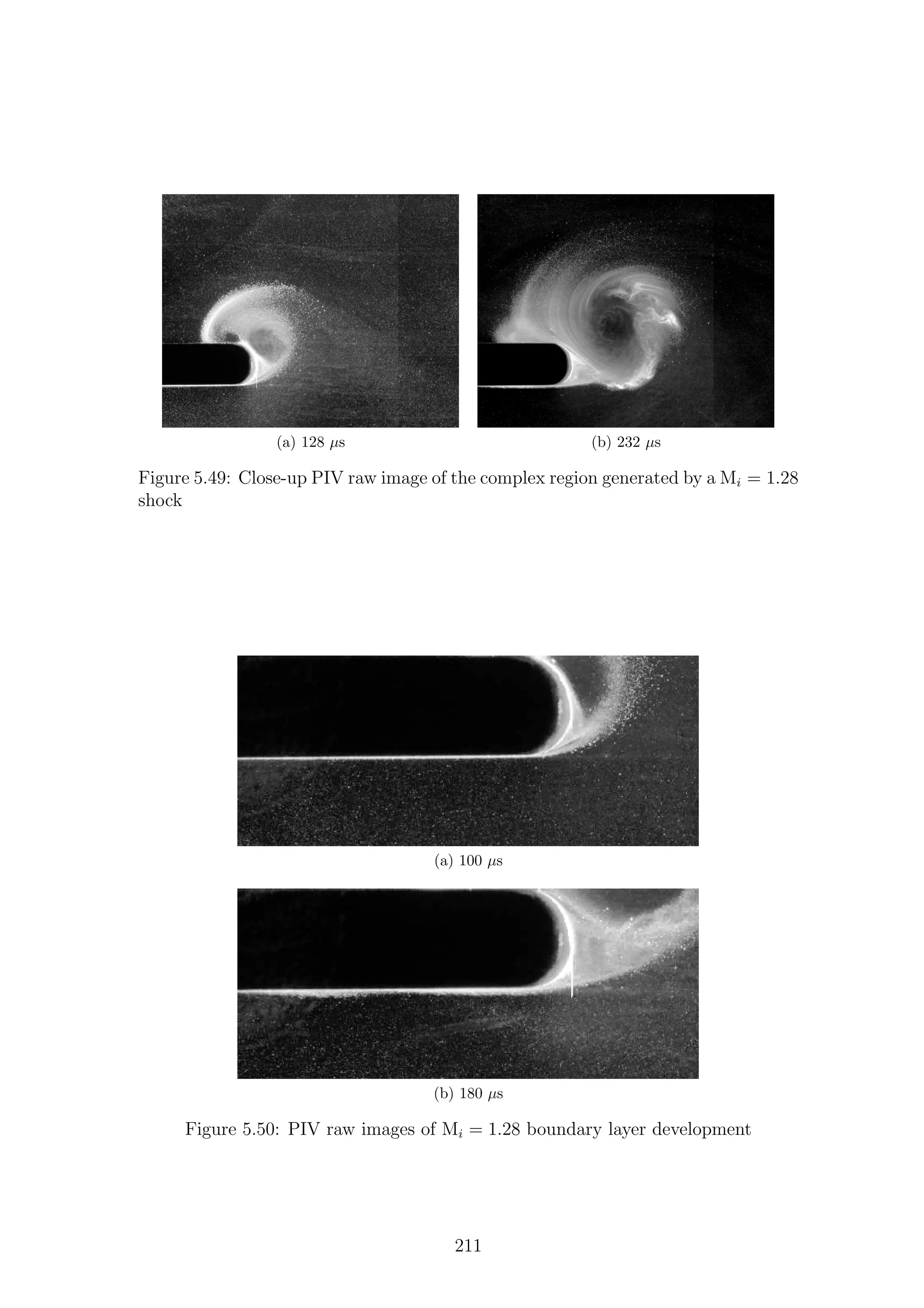
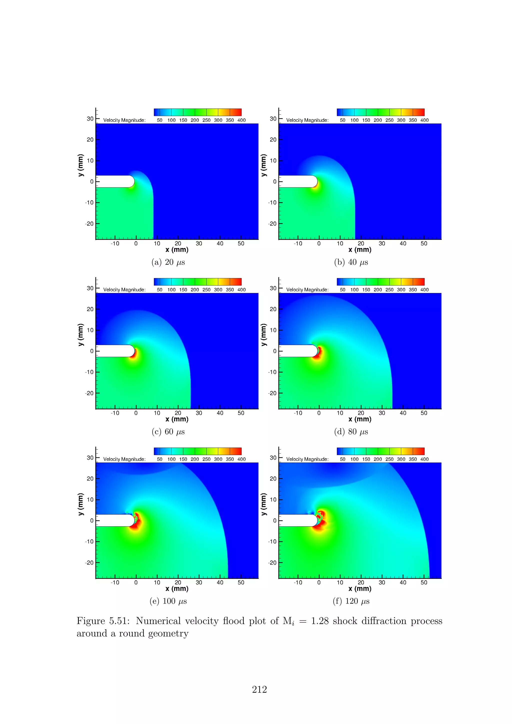
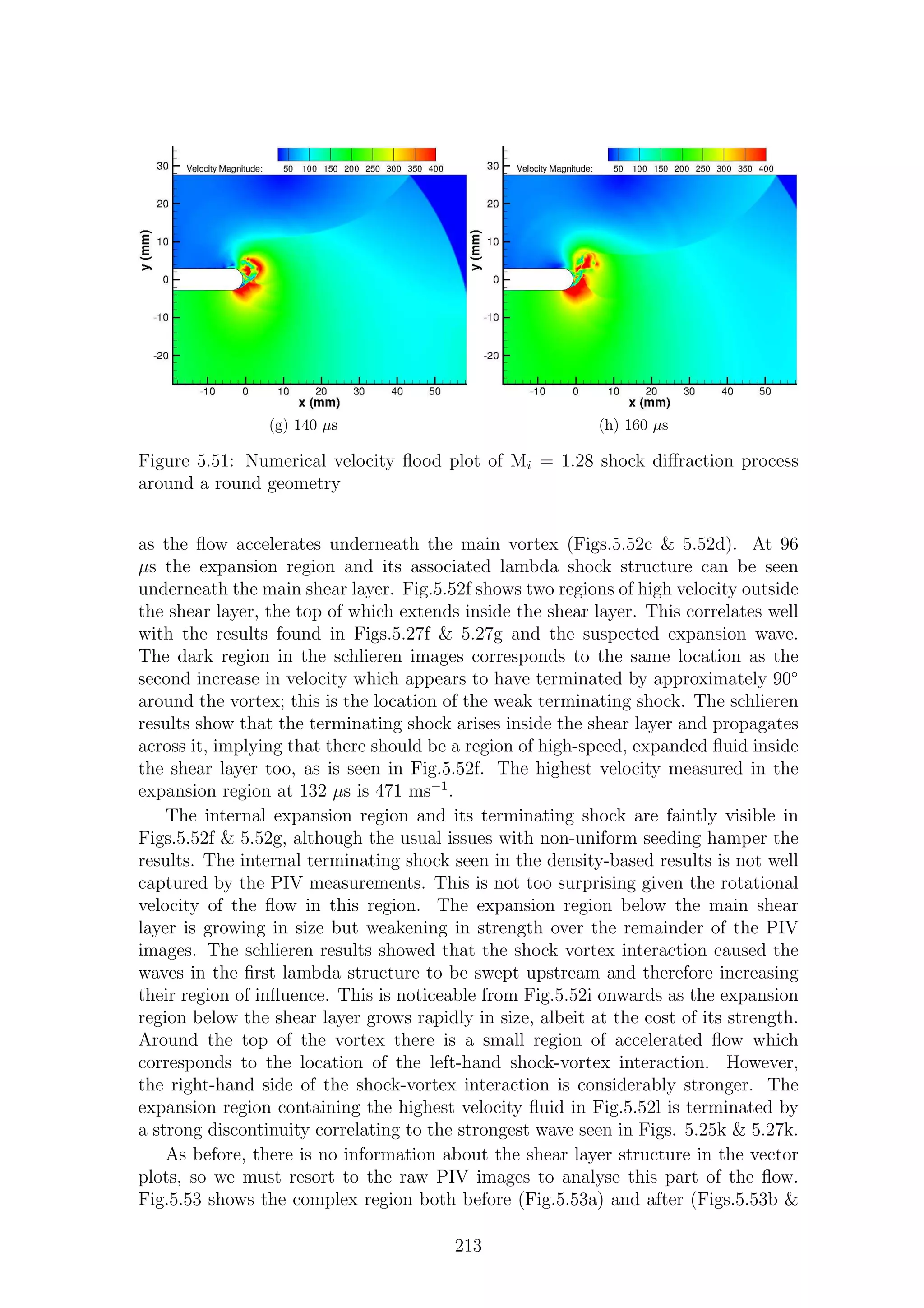
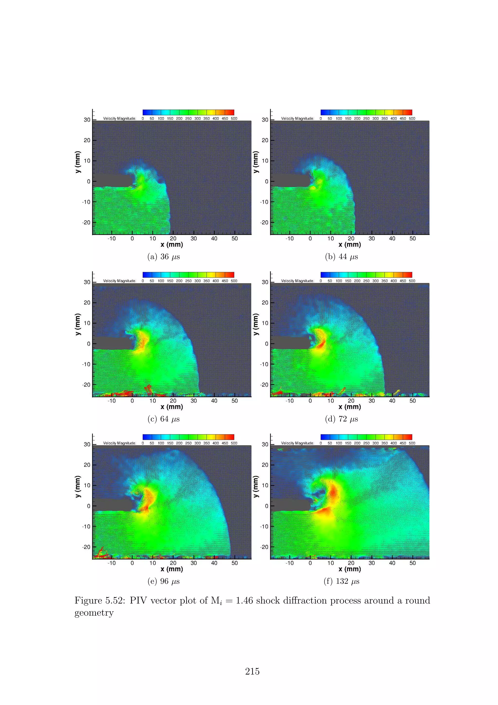
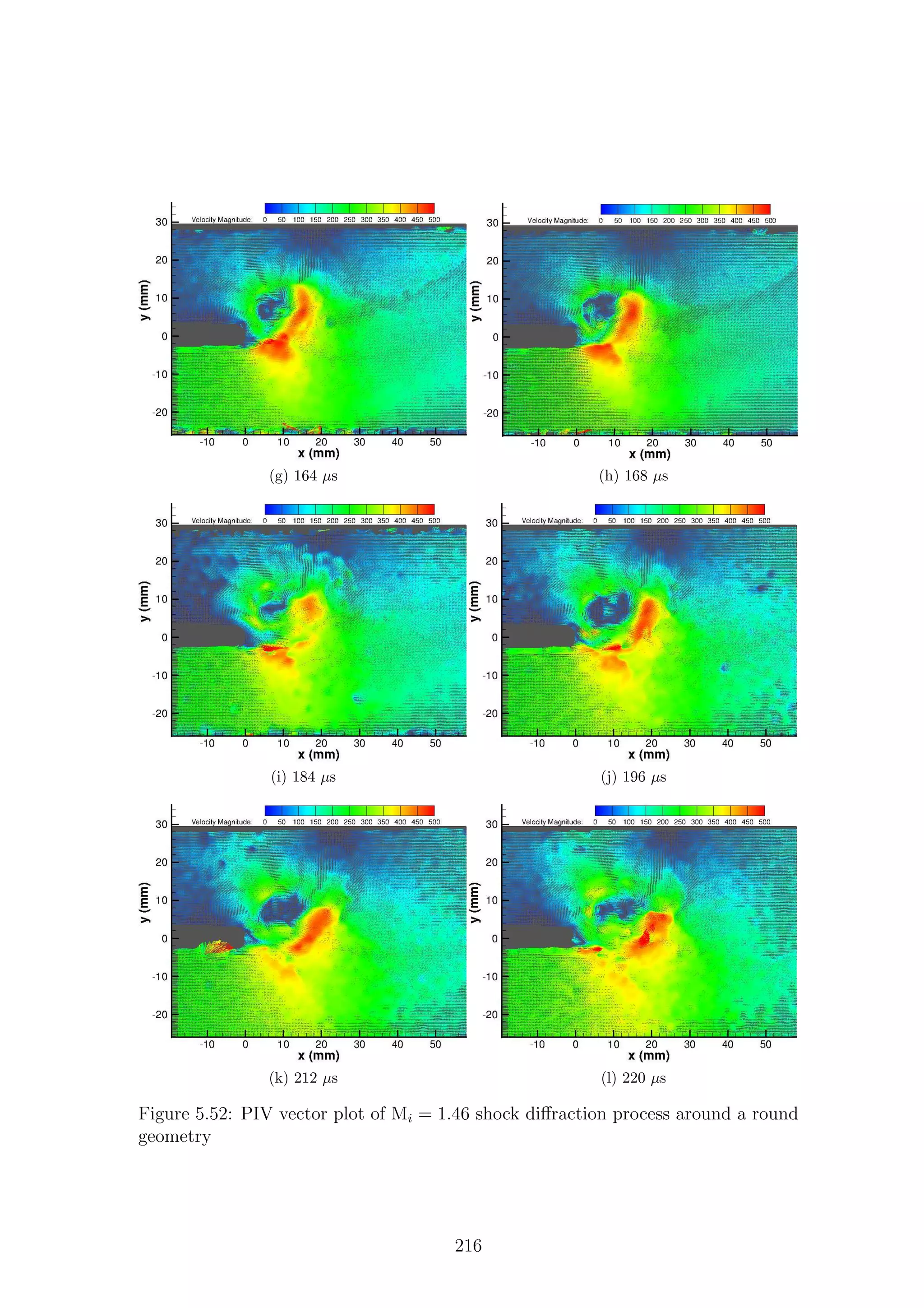
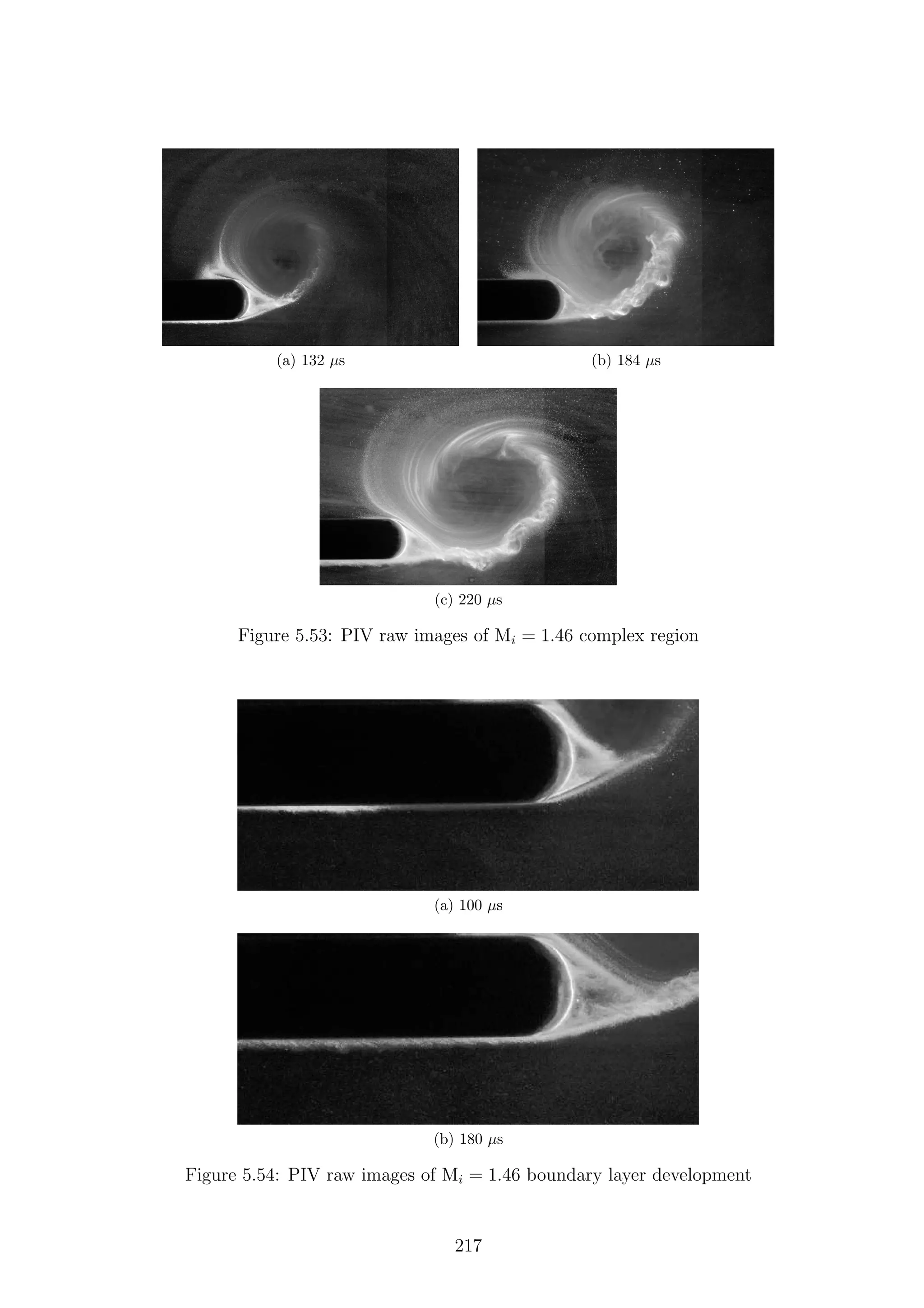
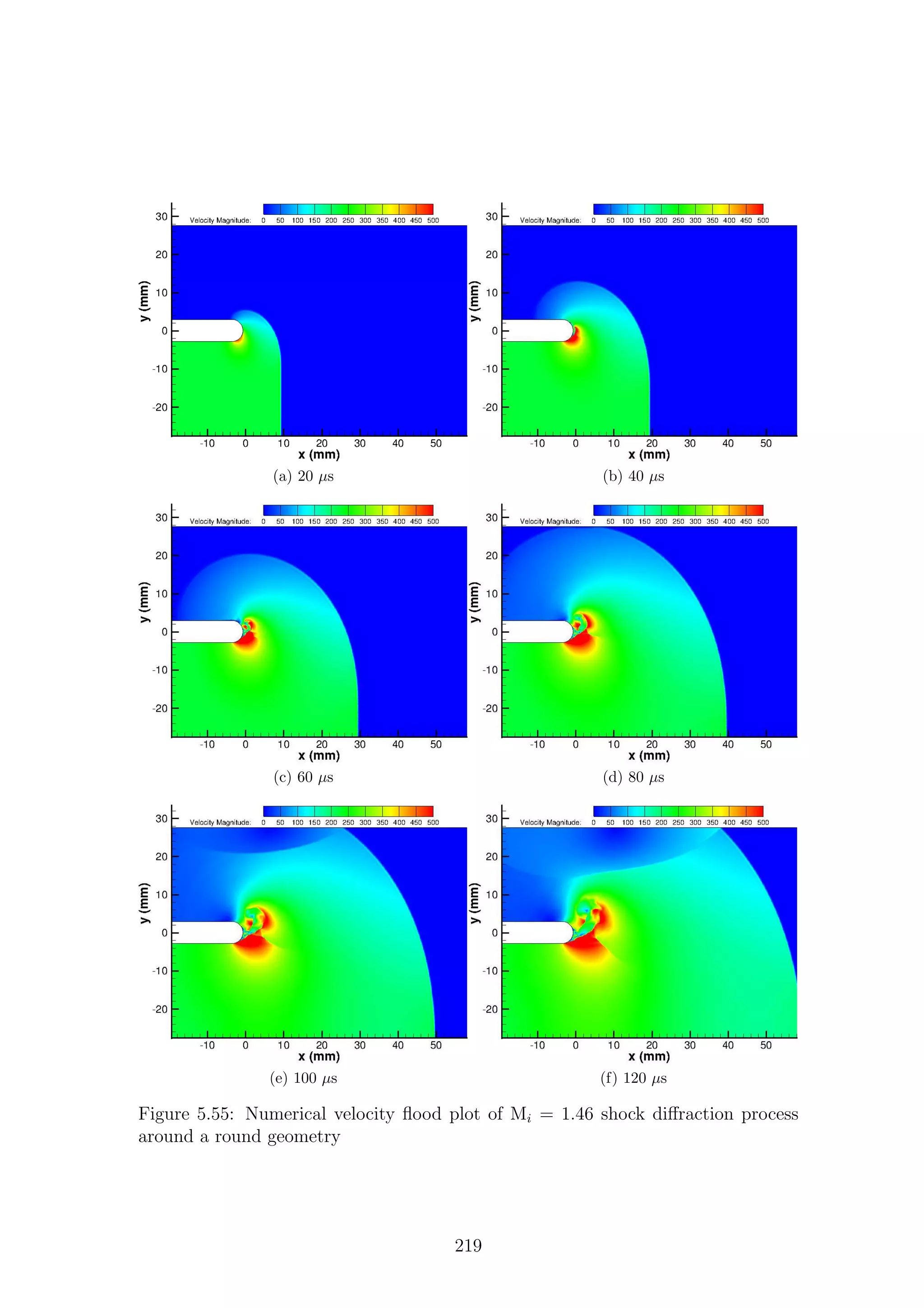
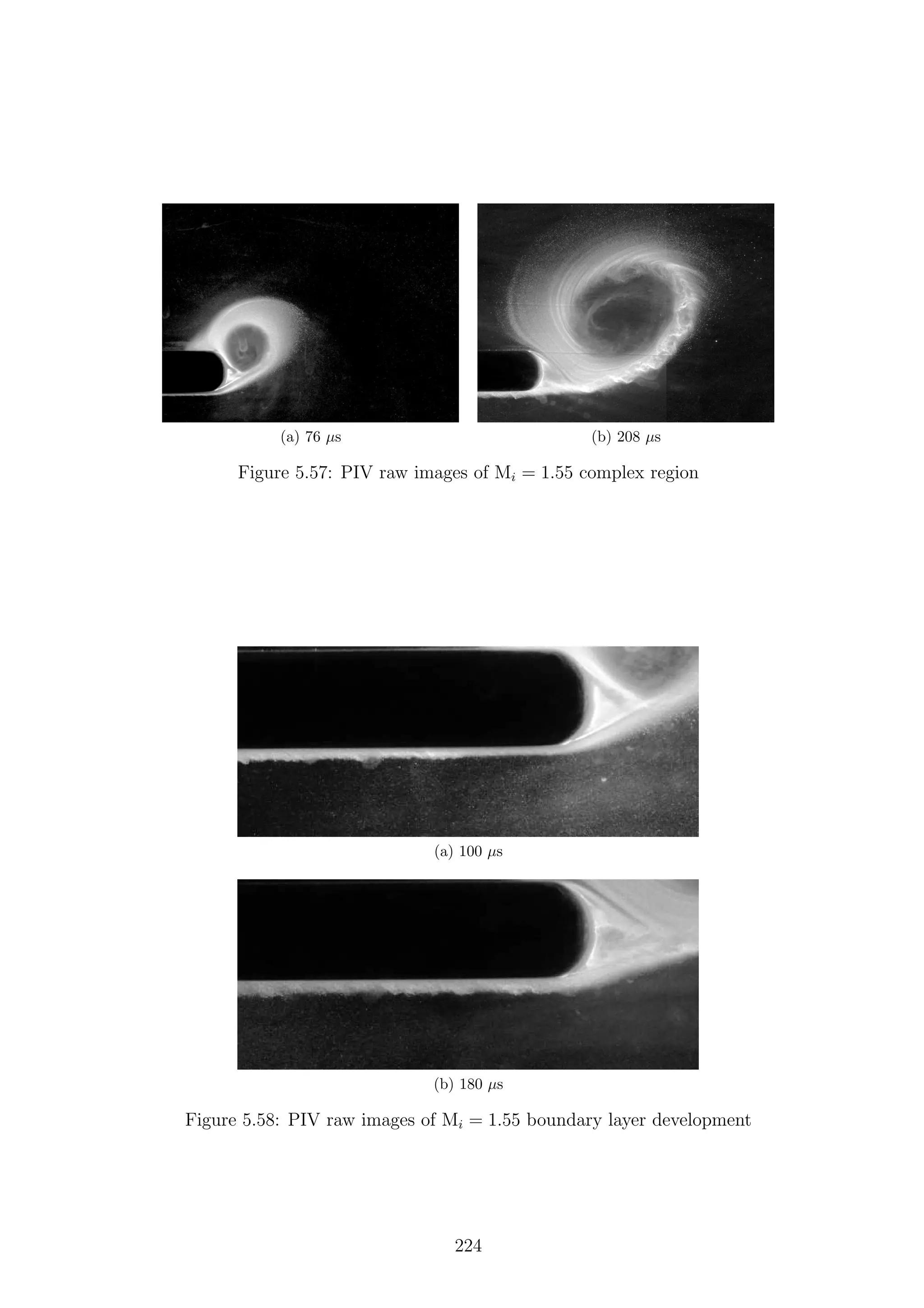
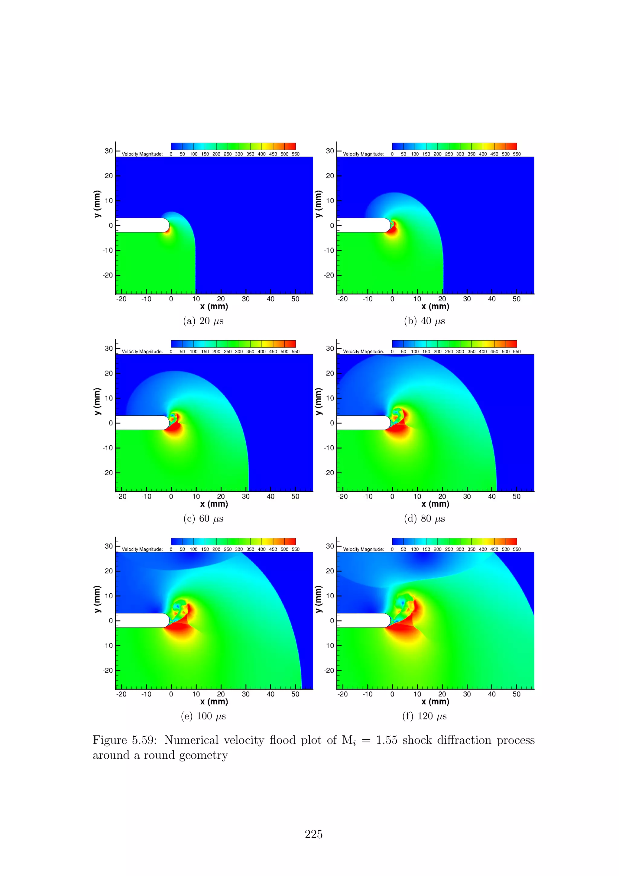
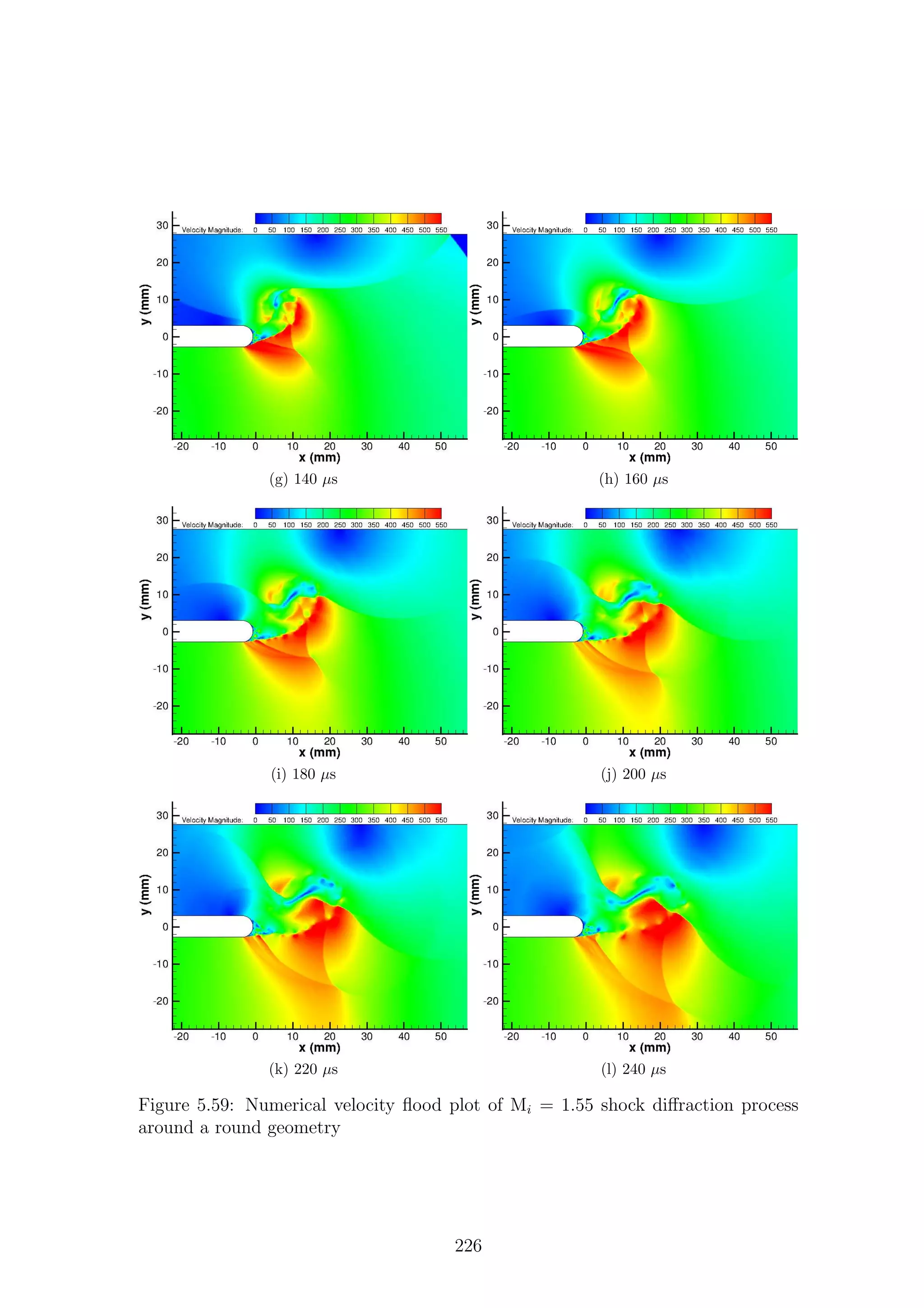
![The Mi = 1.46 case showed a very strong expansion region terminated by a
lambda shock, with a further expansion region after it. This was captured both
experimentally and numerically. As the flow grows faster in time for higher Mach
numbers, the Mi = 1.55 case showed the lambda structures even more clearly. The
secondary expansion region was well captured, as was the shock vortex interaction.
The problem of acquiring measurements in vortex cores is still an unresolved issue.
The proximity of the internal expansion region to the vortex core means that we are
extremely unlikely to obtain reliable quantitative data in this region. However, as
the numerical simulations do not suffer from this problem, they resolved the internal
expansion region well for all three Mach numbers, indicating that the interpretation
of the density-based results is correct.
From the density-based results, it was not possible to conclude much about the
structure of the main shear layer, as there was little visible in the shadowgraph or
schlieren results3
; however, the raw PIV images showed that there are no instabil-
ities present for this geometry like there were for the sharp corner. The numerical
simulations predicted that a series of K-H style vortices would be present on the
shear layer; however, the raw PIV images showed that the shear layer is made up of
turbulent fluctuations. This level of turbulence, not present in the assumptions of
the simulation, gives an extra method of dissipation and damps out the instabilities
from the experimental results.
The incoming boundary layer is not visible in the density-based results section;
however, the raw PIV images highlight it well and allow us to see an instantaneous
snapshot of the structure of the boundary layer. The size of the boundary layers is
such that it was not possible to gain quantitative data from the results presented
here; a different experimental setup would be required and, as the flow is transient,
it would be unnecessary, and probably impossible, to gain statistical data about the
fluctuations in the boundary layer. The raw PIV images show the growth of the
boundary layer and some results indicate that there are structures aligned at ap-
proximately 45◦
to horizontal. These structures are likely to be packets of vorticity,
possibly in the form of hairpin vortices, similar to those seen by Adrian et al. [200].
3
This has been the case for many researchers in the past looking at similar problems to this;
therefore more conclusive evidence is needed.
227](https://image.slidesharecdn.com/4a6f74b5-6bbb-4ffd-b3f5-7486cdb057cd-150303082443-conversion-gate01/75/Mark-Quinn-Thesis-258-2048.jpg)
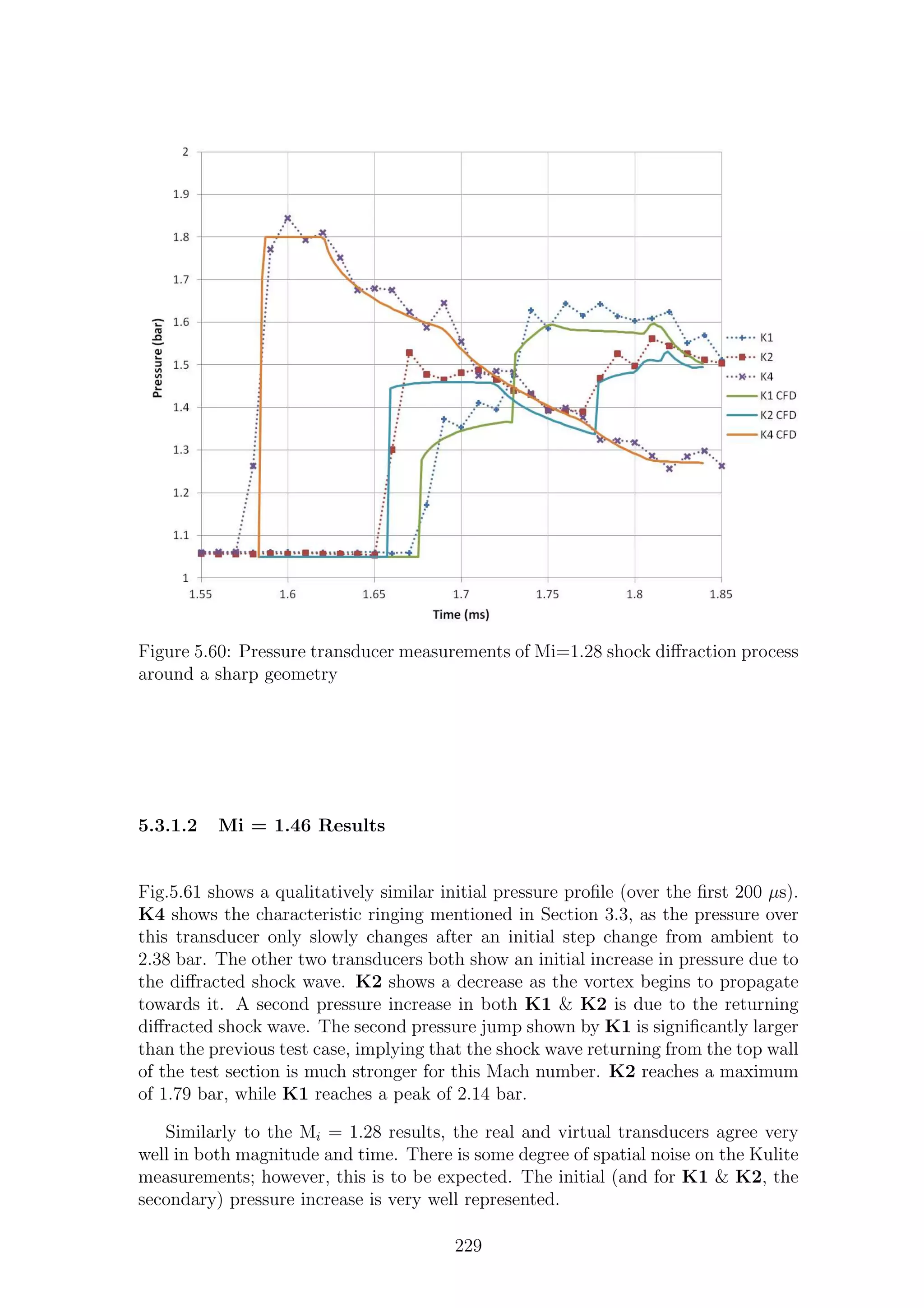
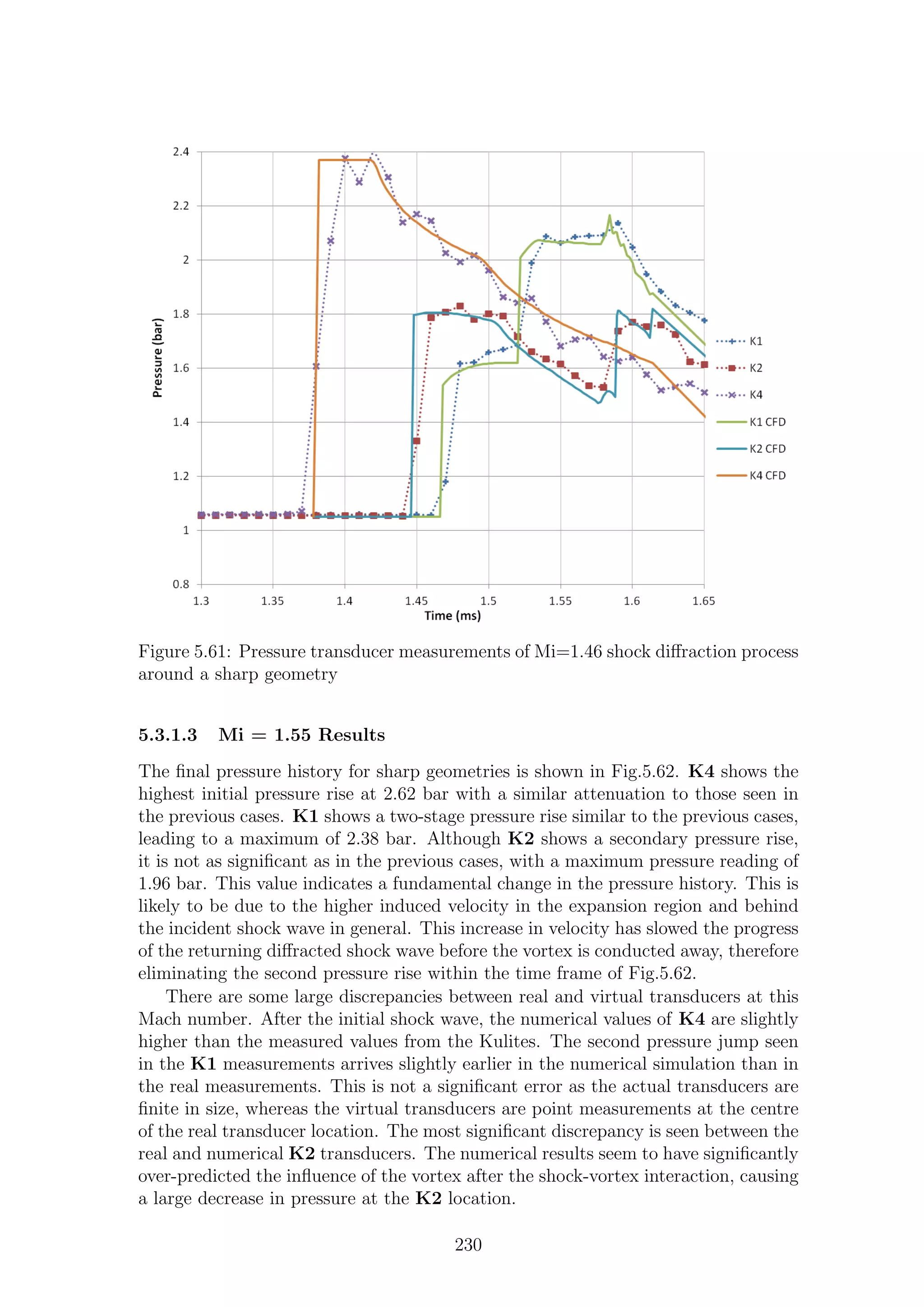
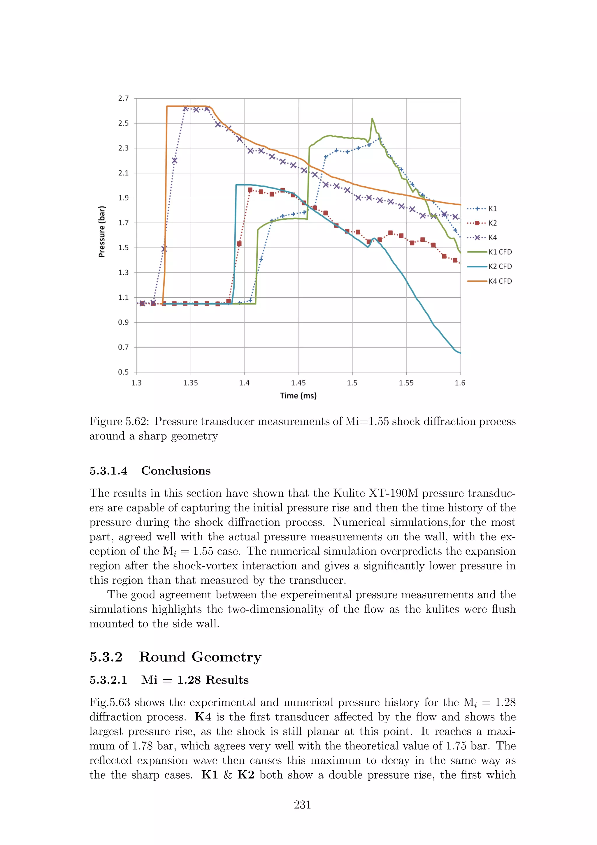
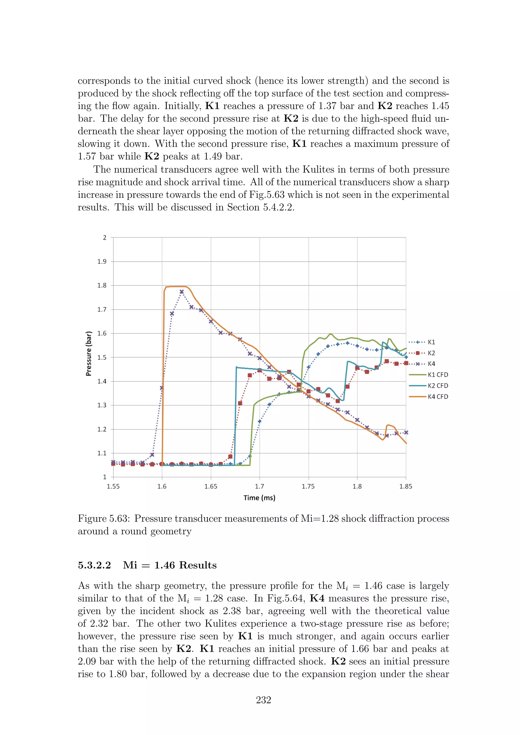
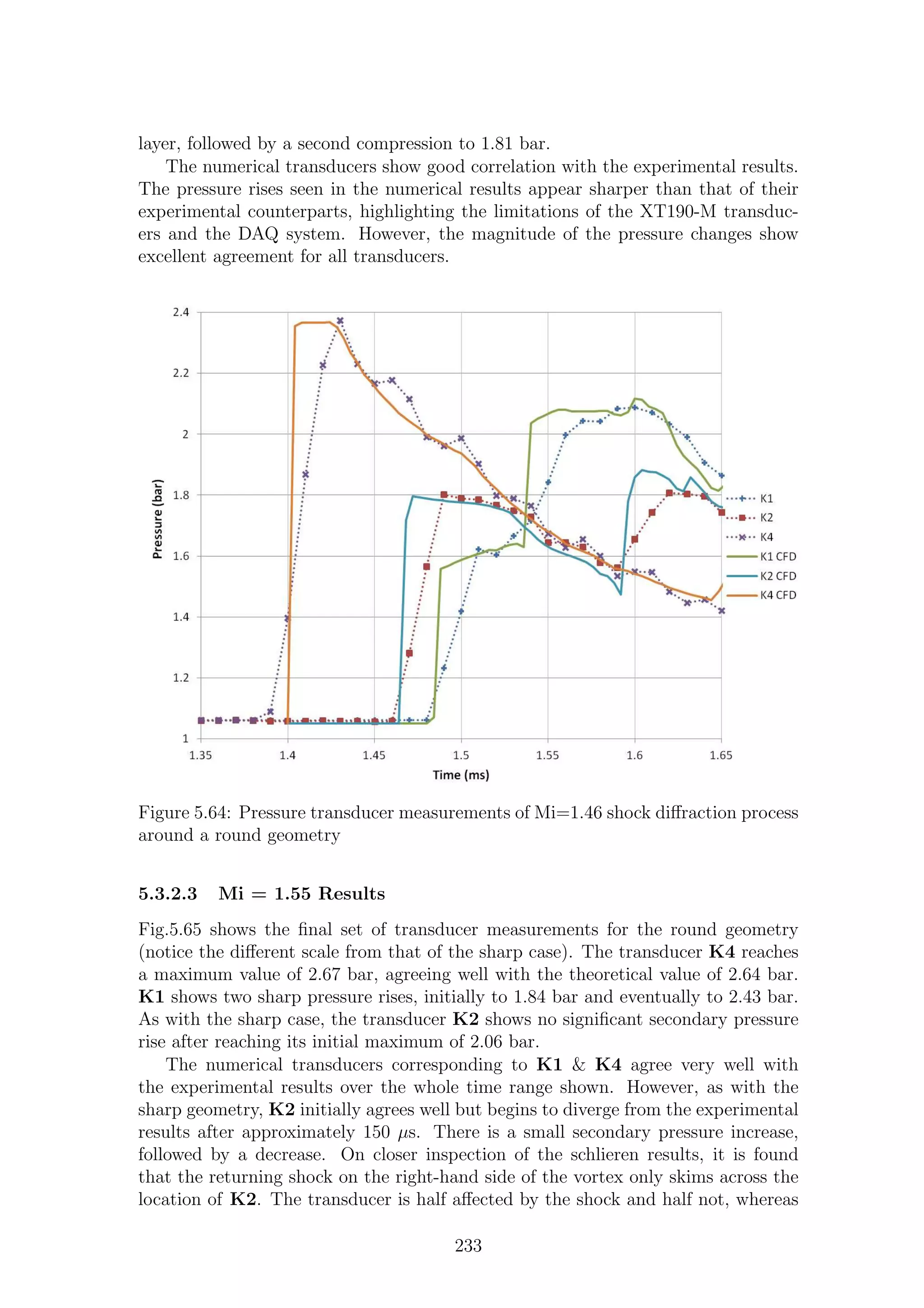
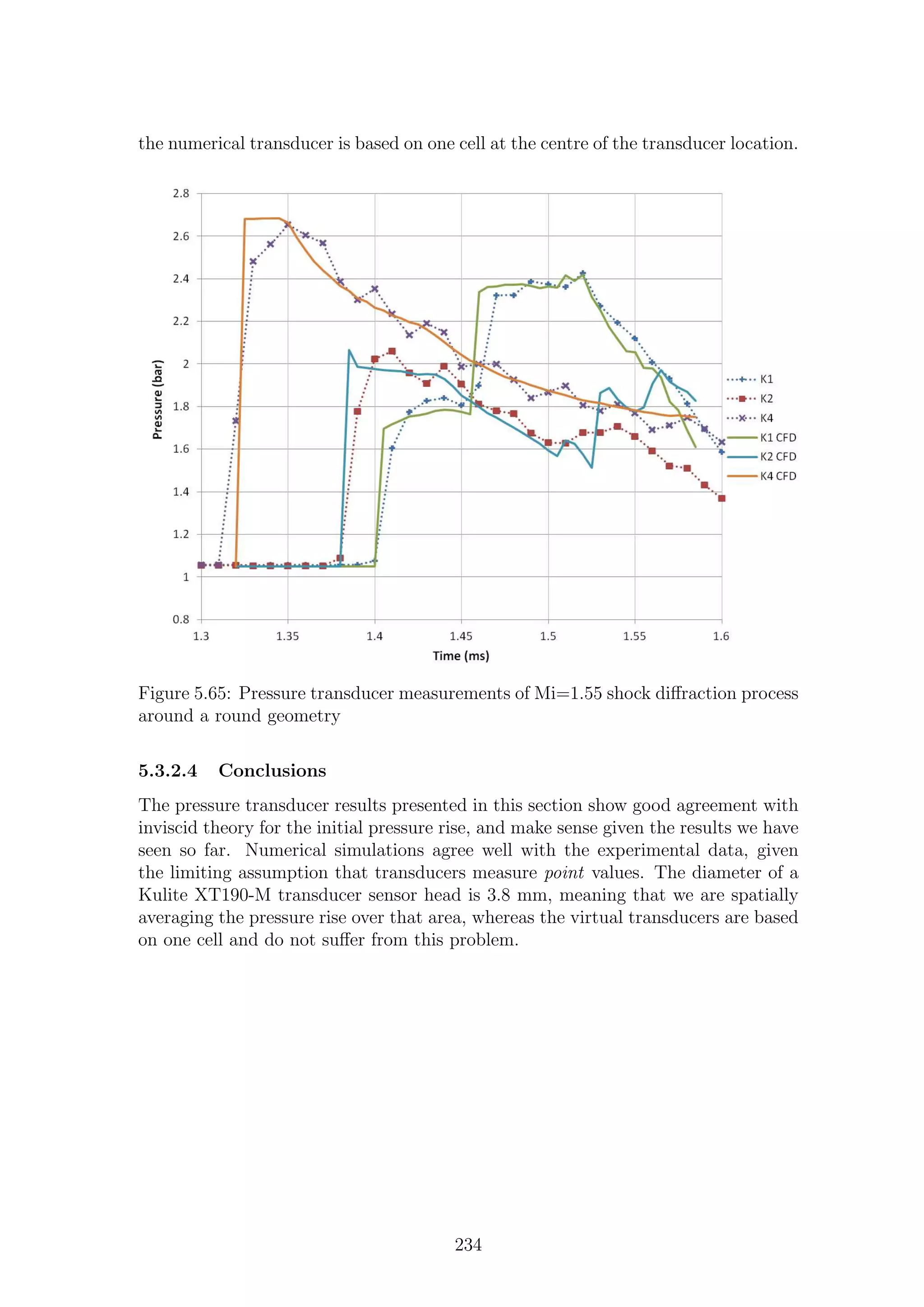
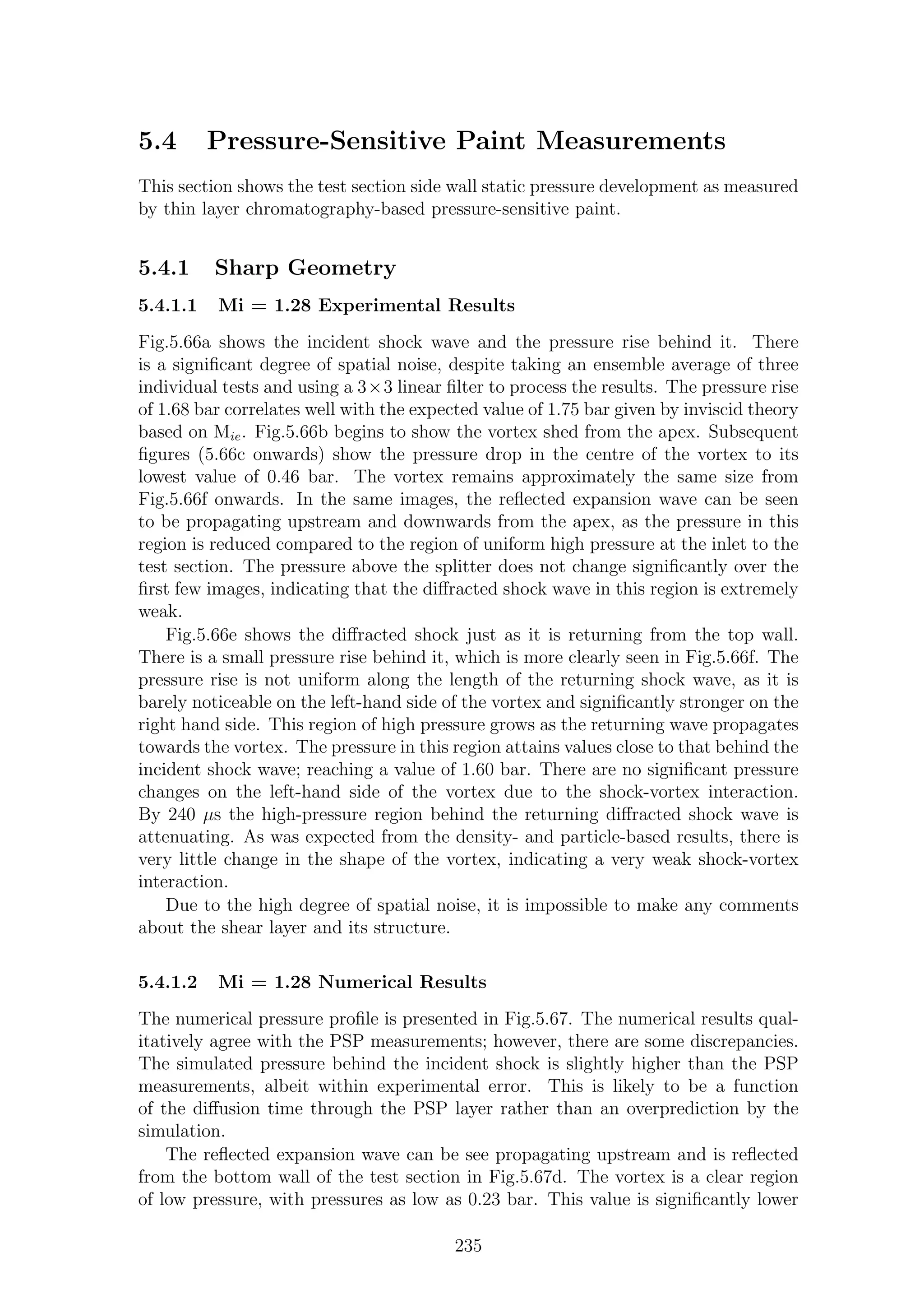
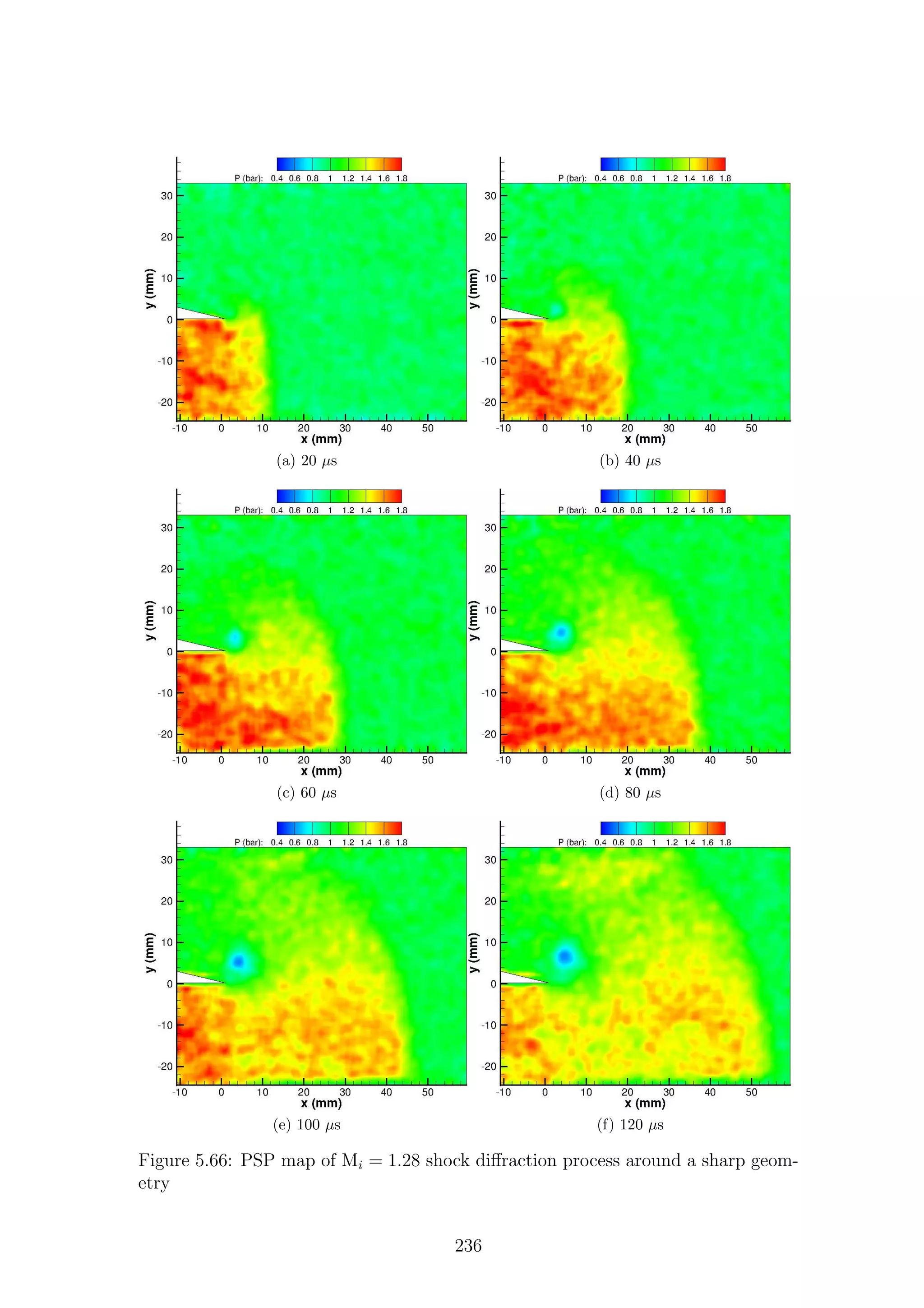
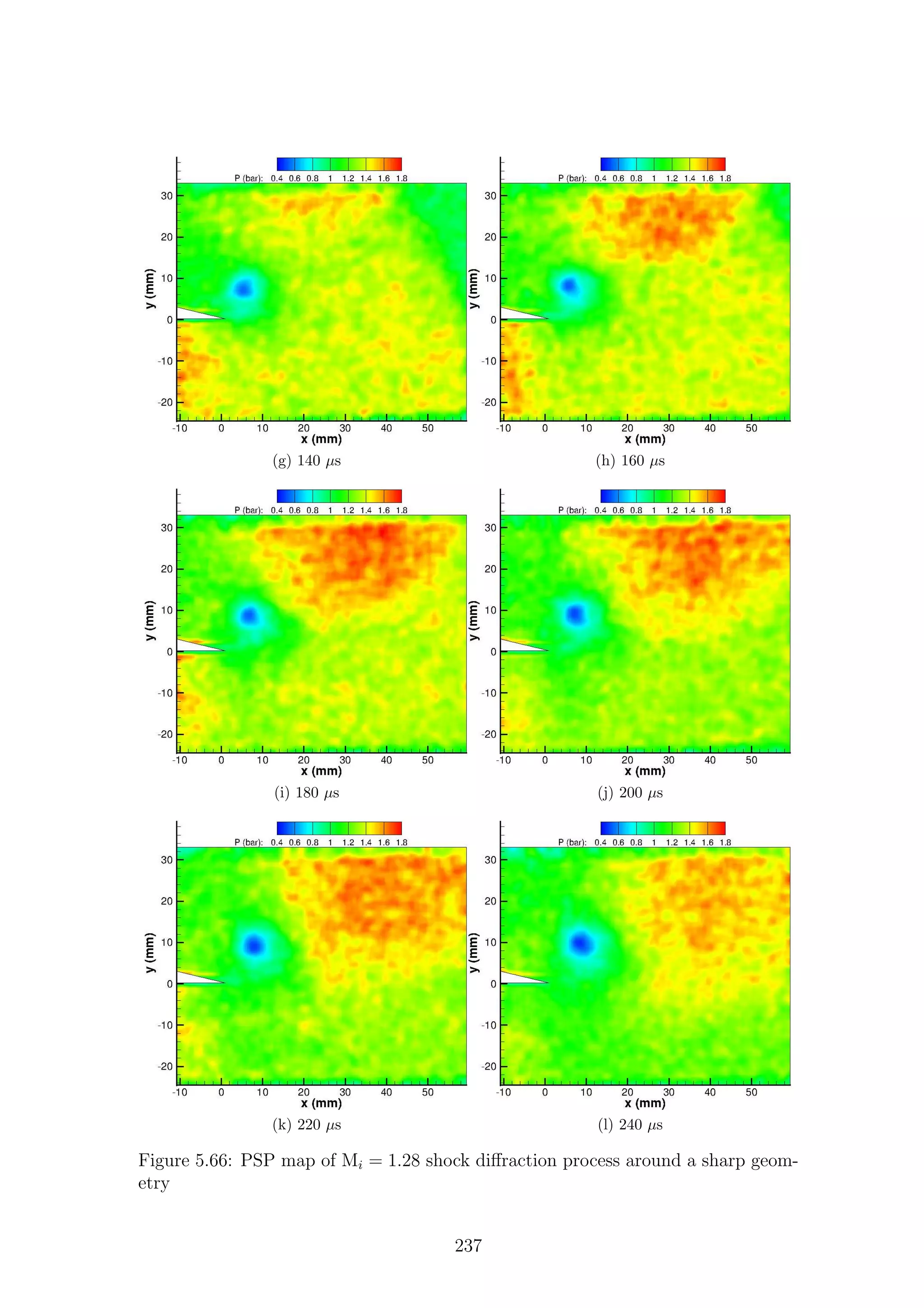
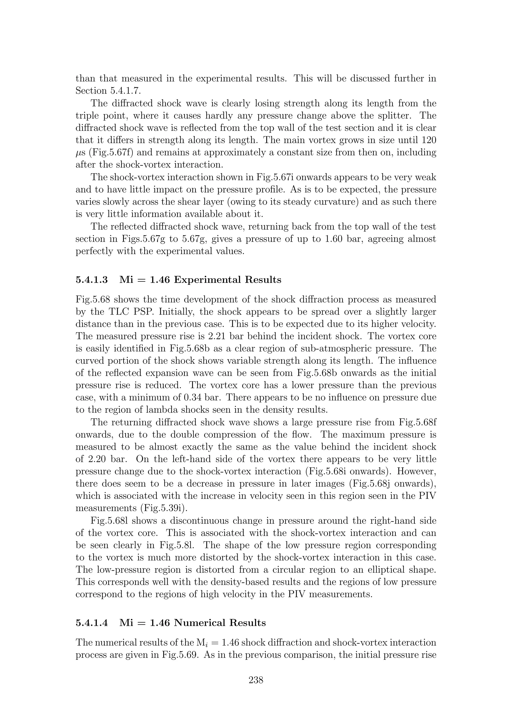
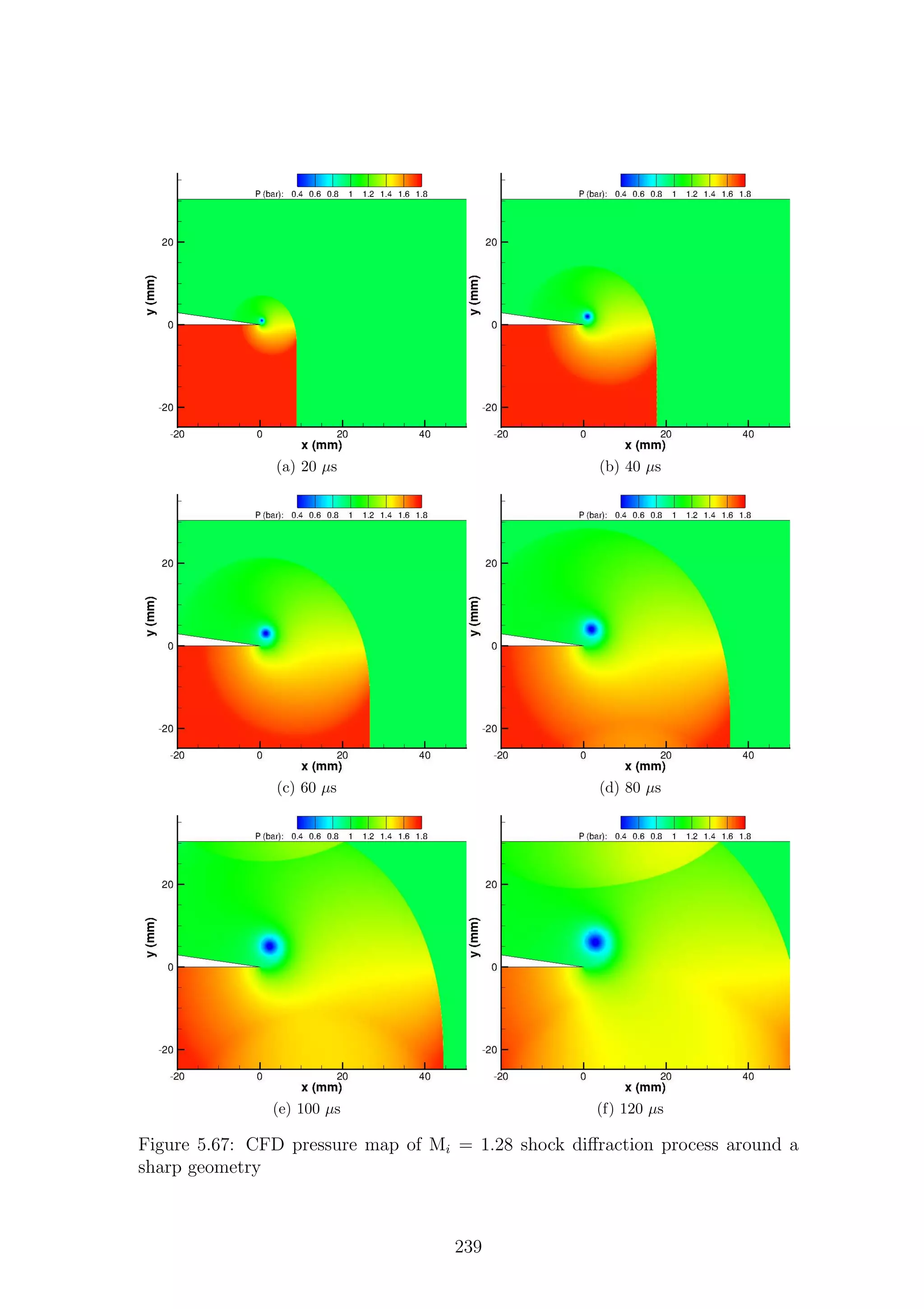
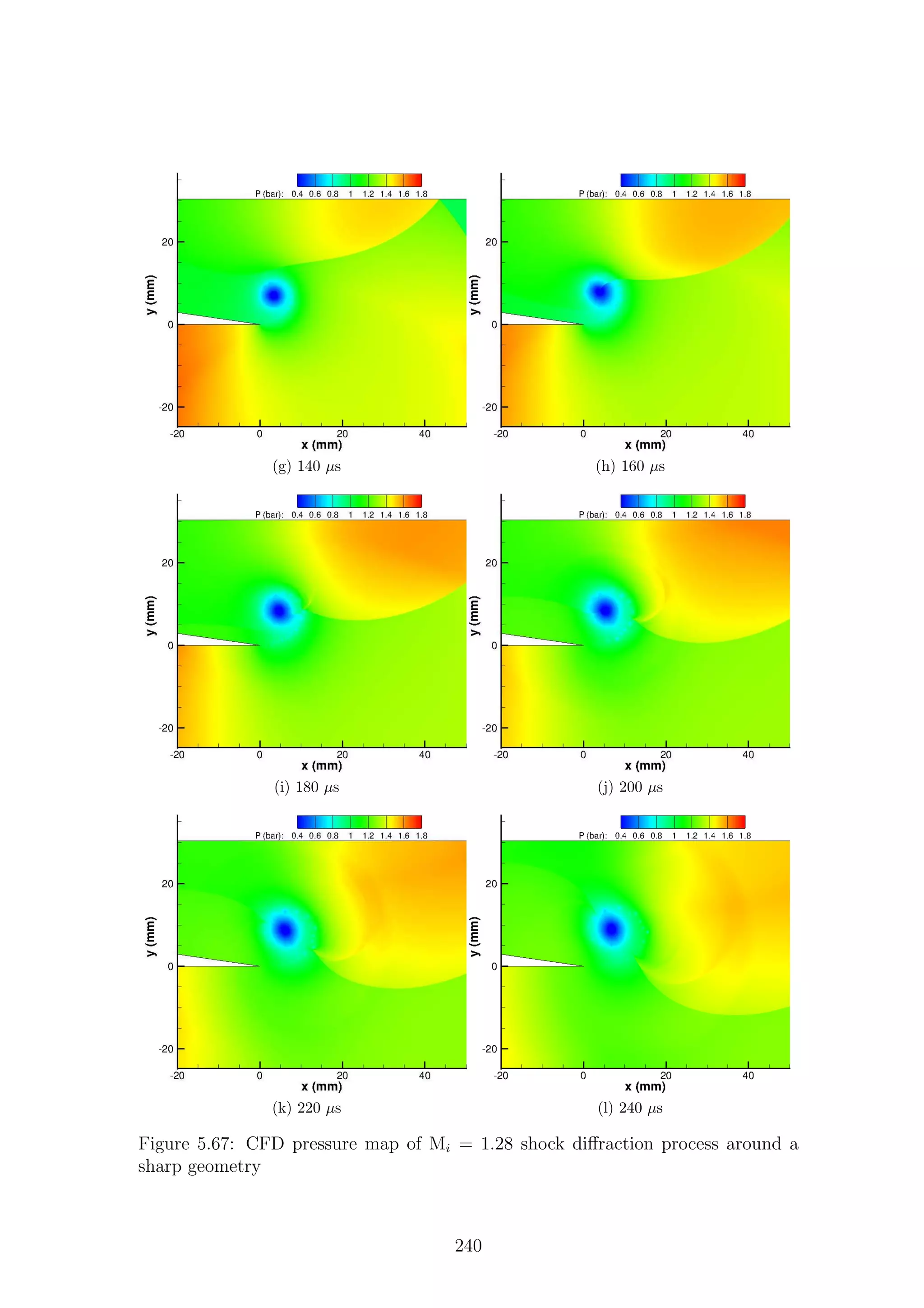
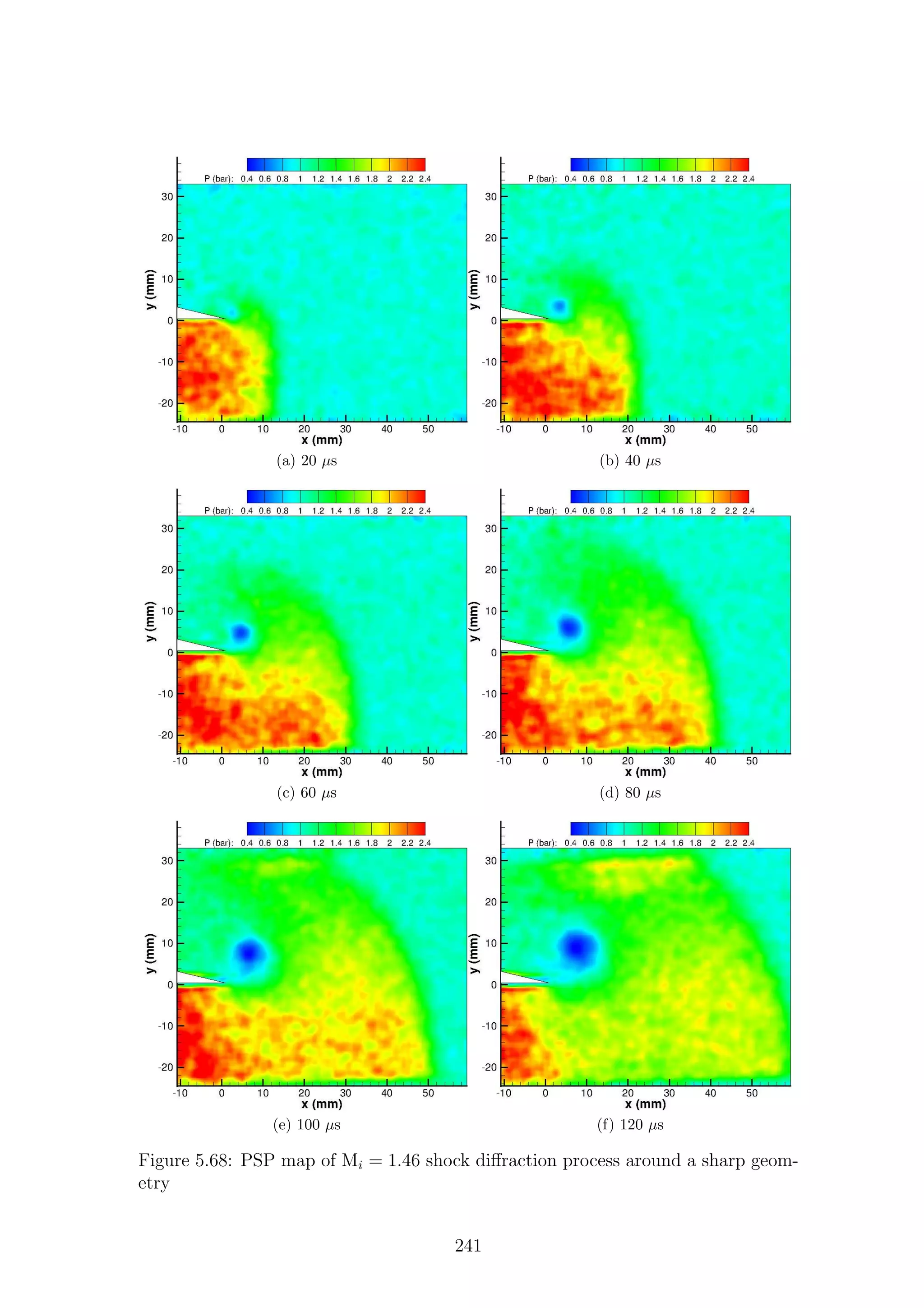
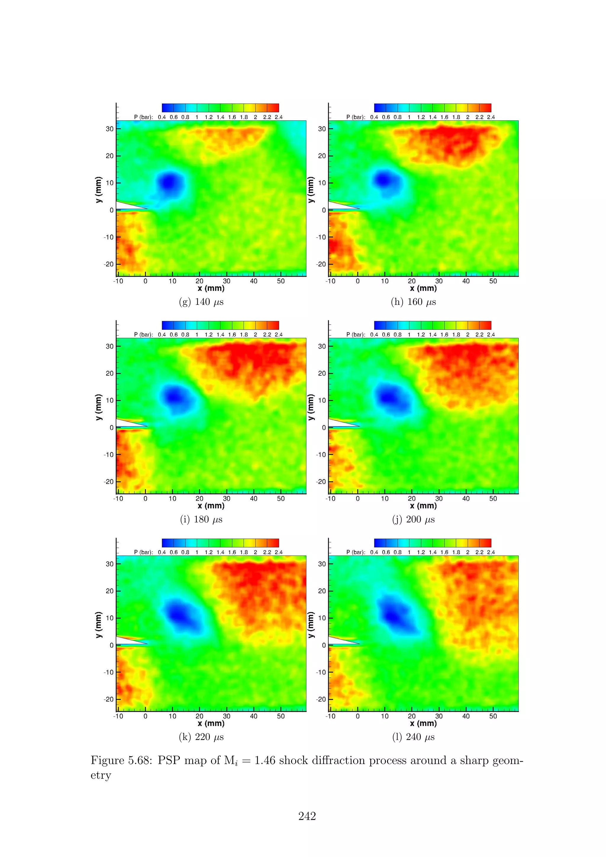
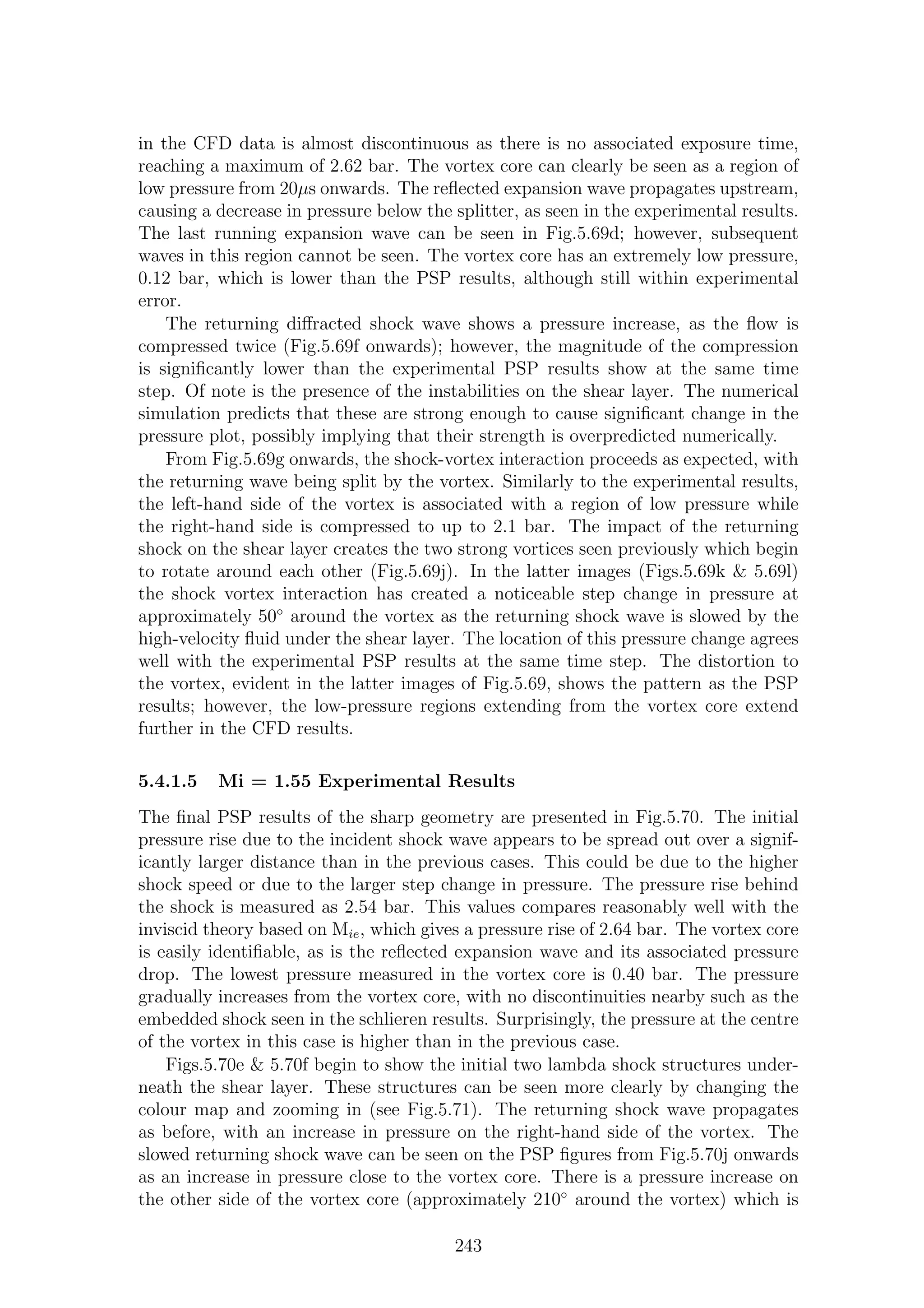
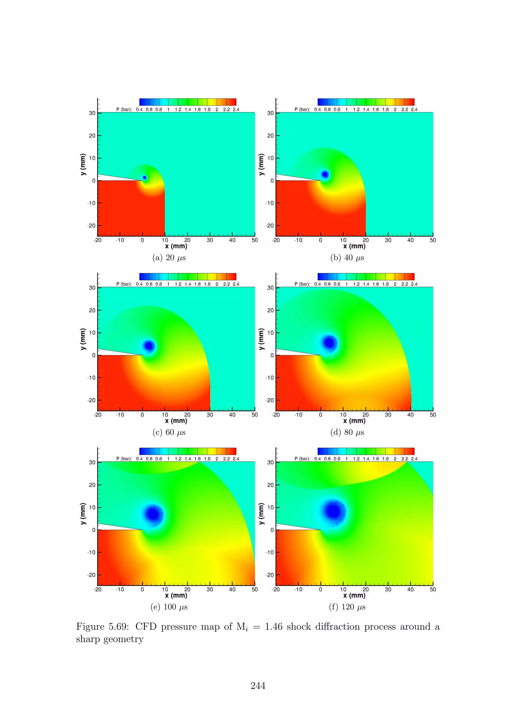
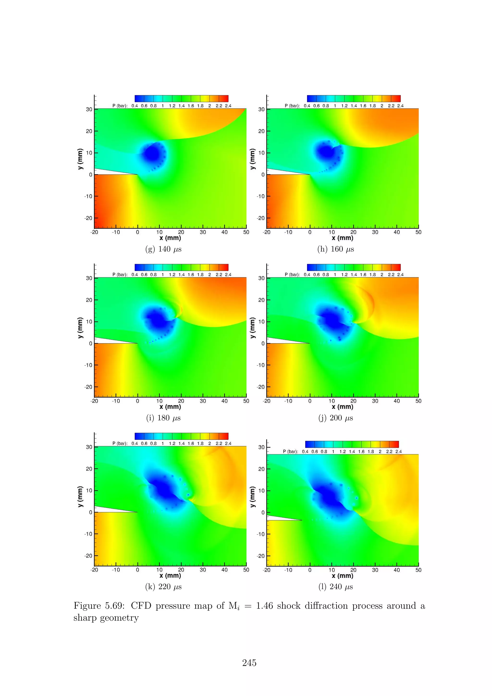
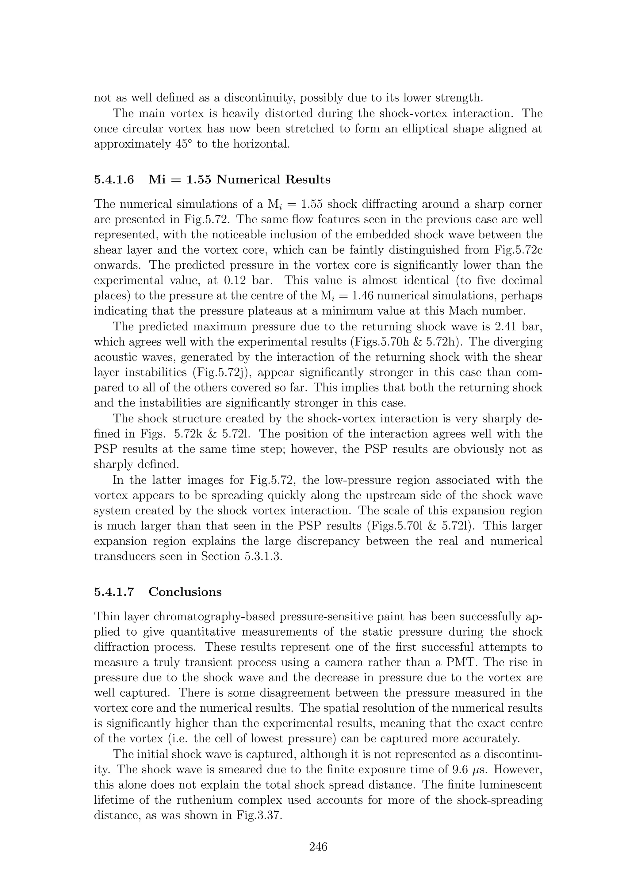
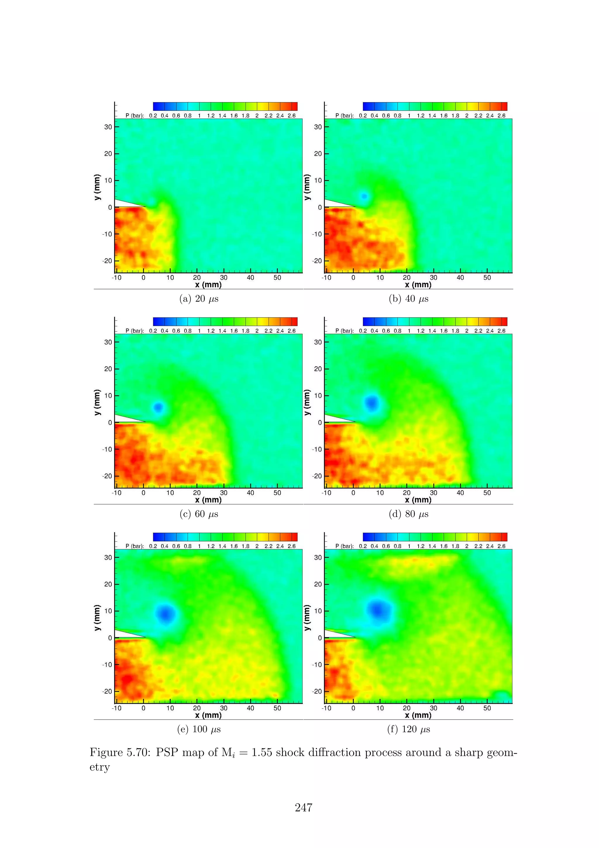
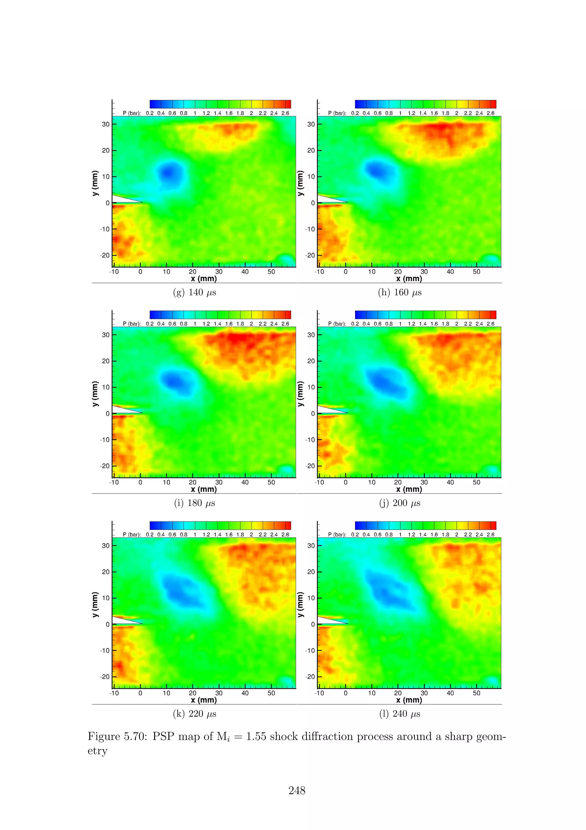
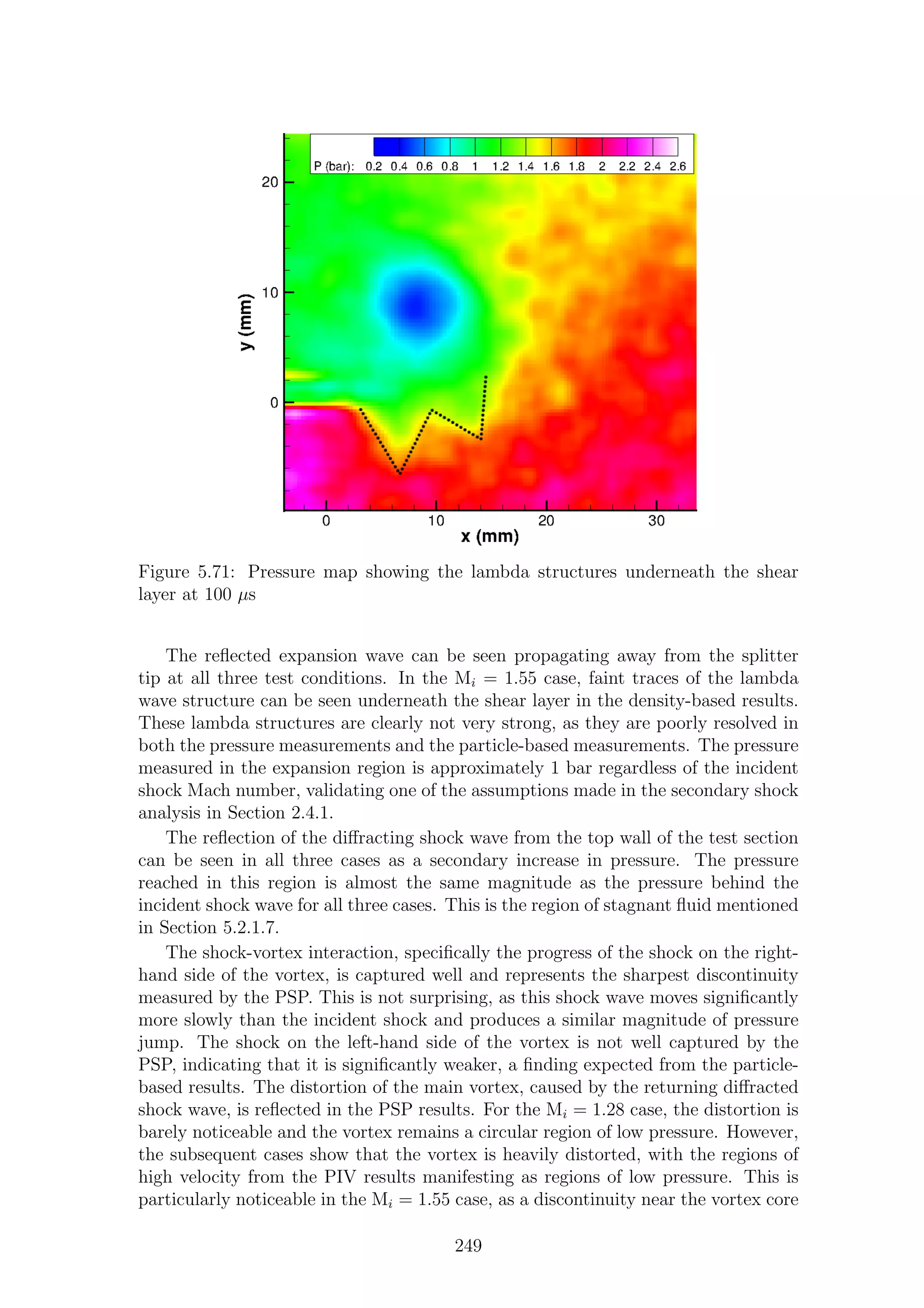
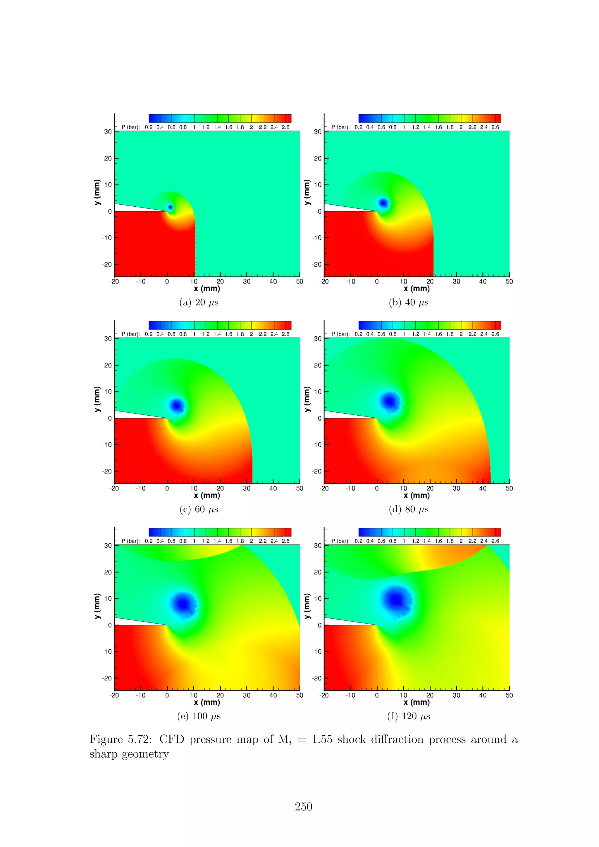
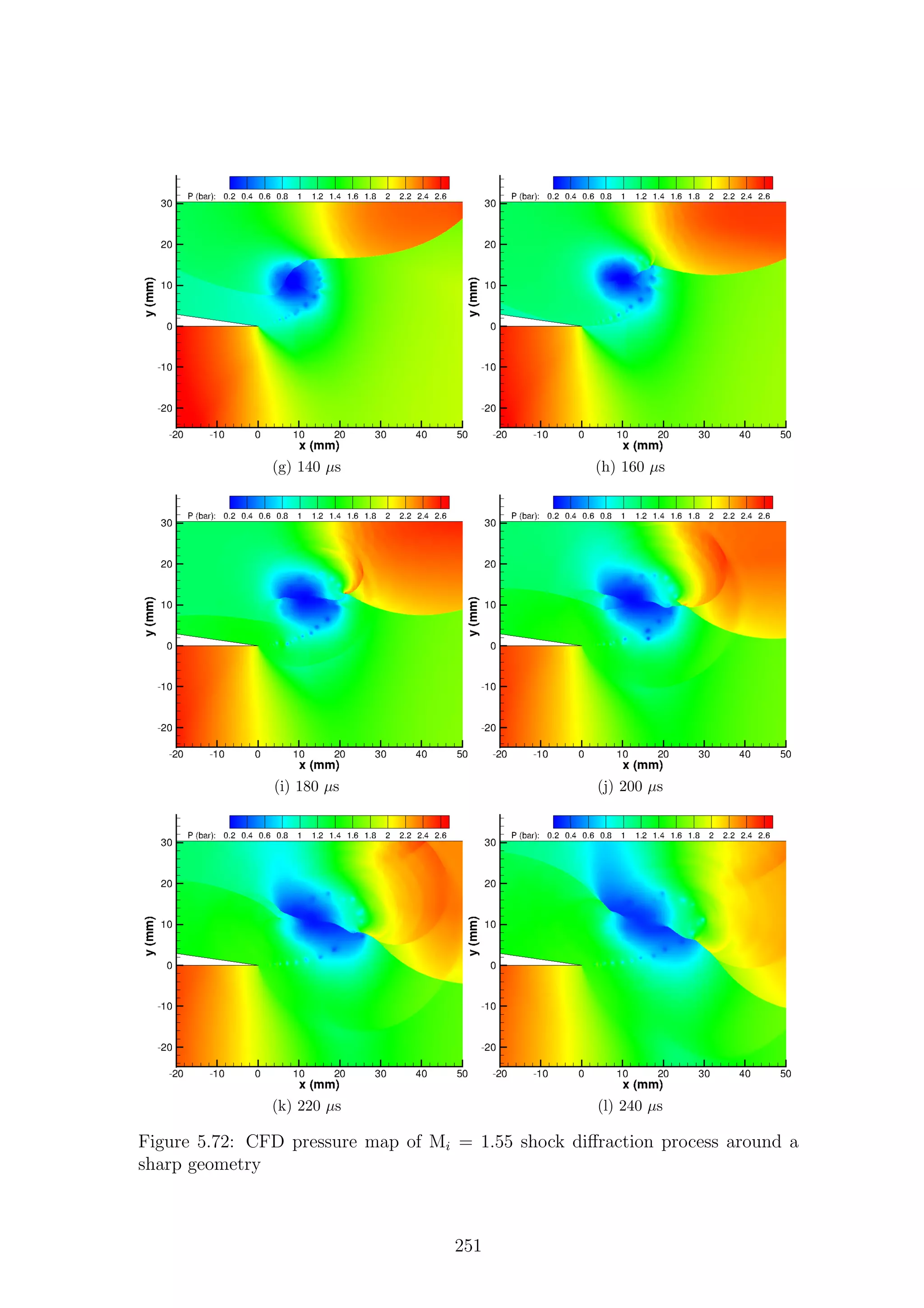
![can be seen. The pressure spike seen by Skews et al. [71] is not seen in either the
numerical or experimental results.
The low spatial resolution of the PSP results and relatively high degree of spatial
noise means that no information can be gathered about the shear layer. It would be
expected that, initially, where the shear layer is straight, the pressure on either side
would be equal, meaning that PSP would not give significant information. To begin
with, the same is true in the numerical results; however, eventually the instabilities
on the shear layer become strong enough to manifest themselves in the static pressure
field.
There is a significant degree of spatial noise present in the experimental results.
This is primarily due to the shot noise, as was shown in Section 3.4.10. The spatial
noise can only be reduced by ensemble-averaging multiple runs, as it consists of
random fluctuations. Future improvements in CCD technology should also reduce
this problem. Despite the high level of spatial noise, the experimental and numerical
results agree within experimental error, with the exception of the exact vortex core
pressure. The PSP measurements also show that the influence of the low-pressure
region after the Mi = 1.55 shock-vortex interaction is not as strong as the numerical
predictions, agreeing with the conclusion of Section 5.3.1.4. This is likely to be a
numerical error rather than the PSP not responding quickly enough, as the results of
Gregory & Sullivan show that PSP responds to a decrease in pressure more quickly
than to an increase in pressure [184].
252](https://image.slidesharecdn.com/4a6f74b5-6bbb-4ffd-b3f5-7486cdb057cd-150303082443-conversion-gate01/75/Mark-Quinn-Thesis-283-2048.jpg)
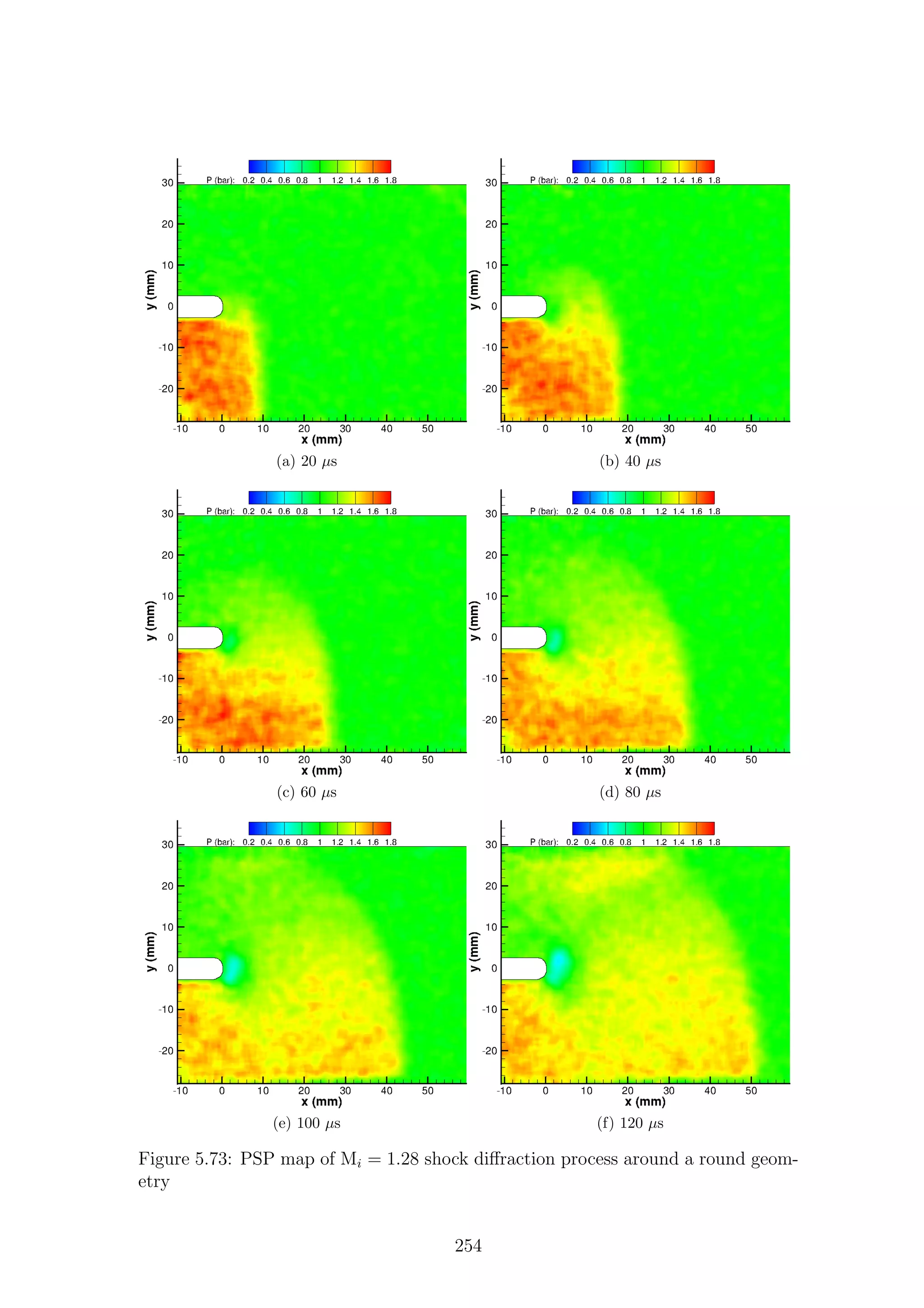
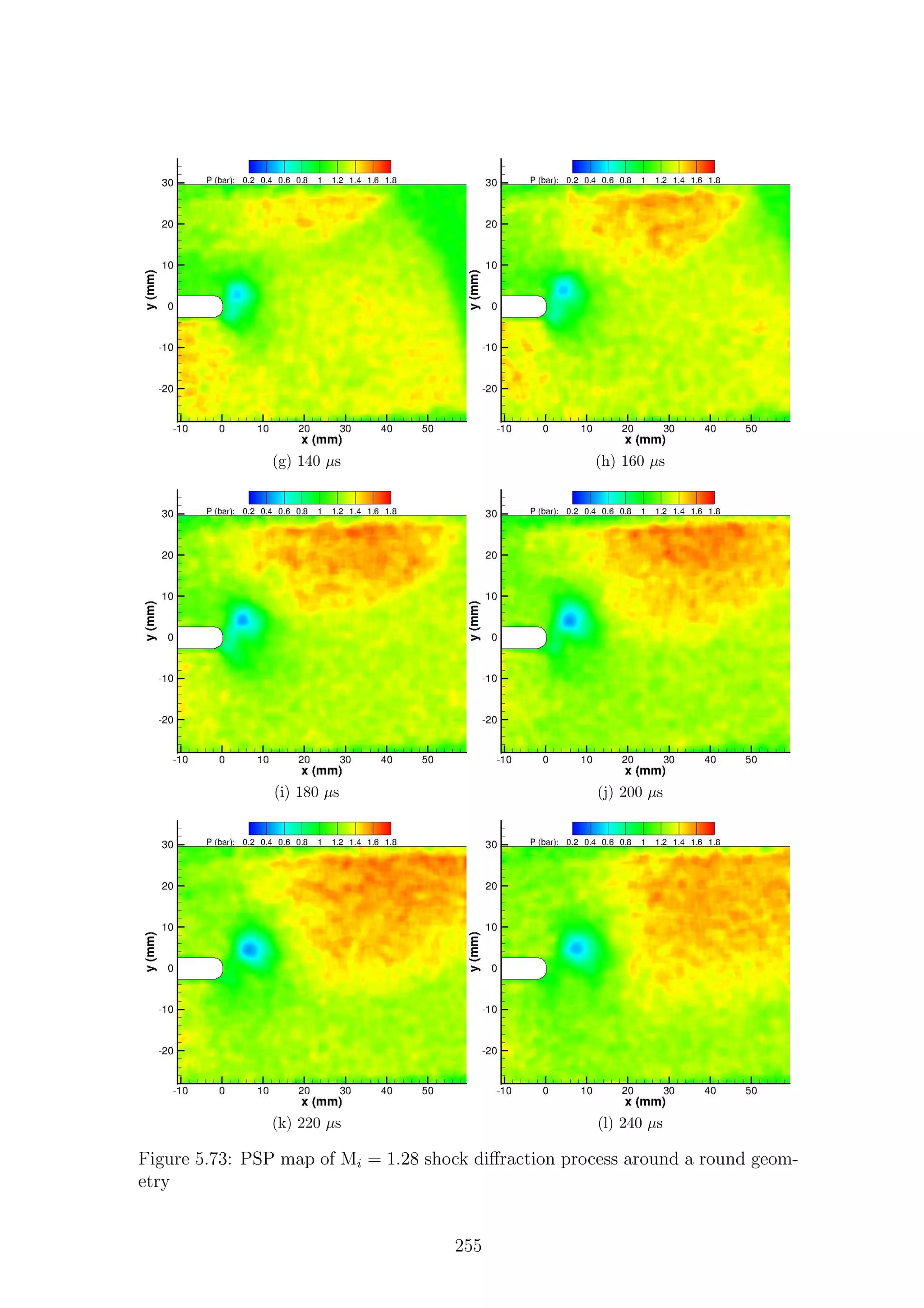
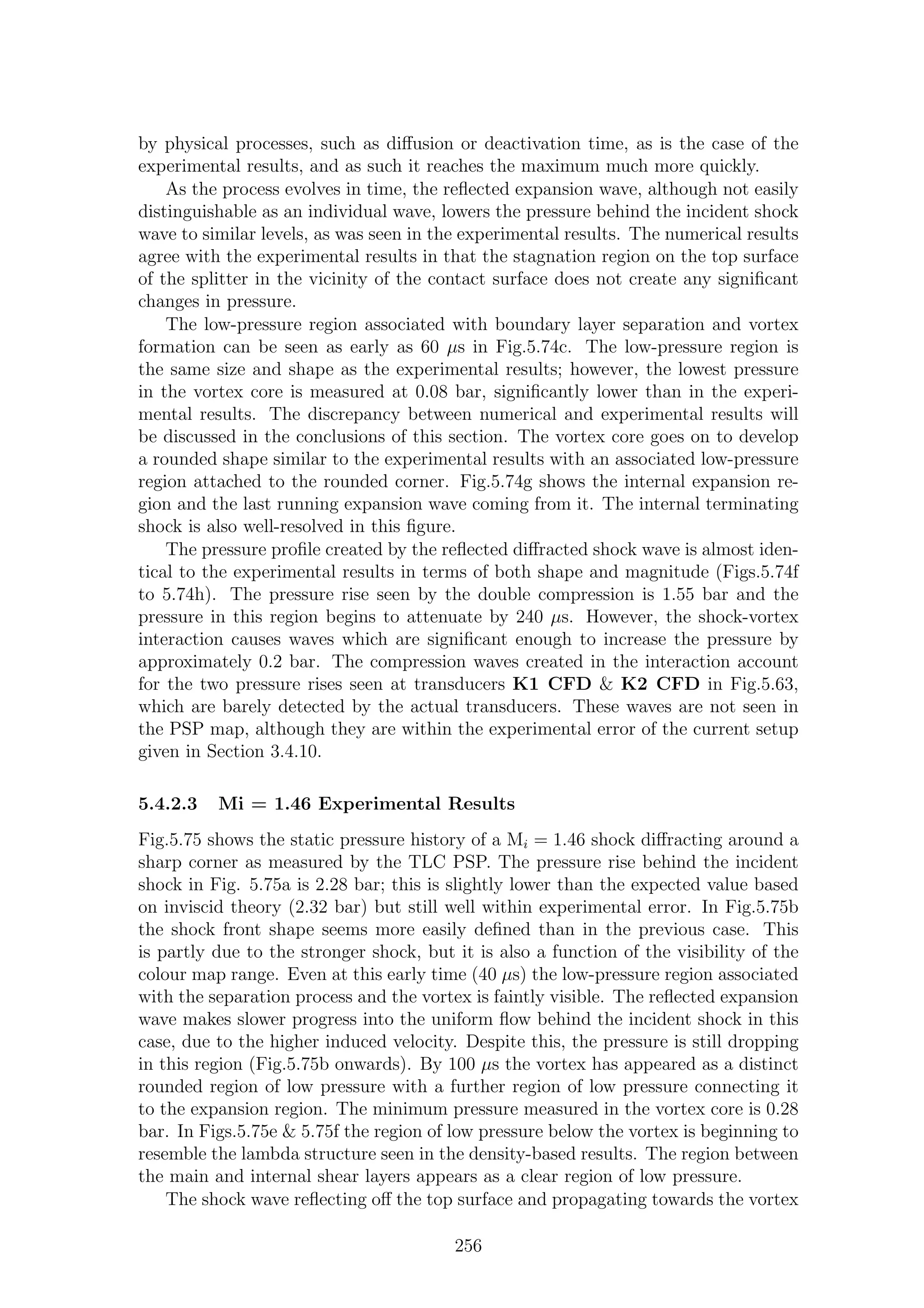
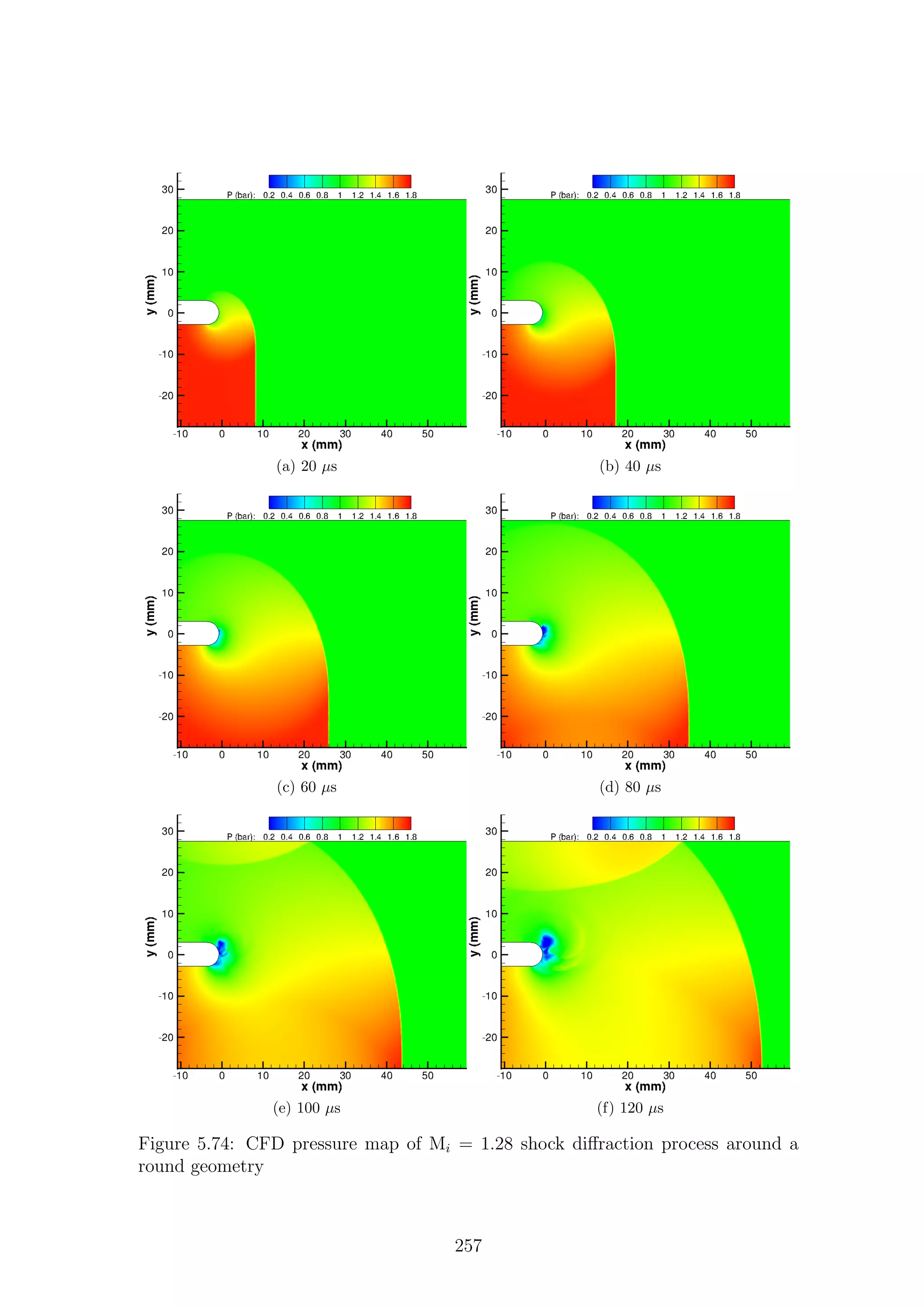
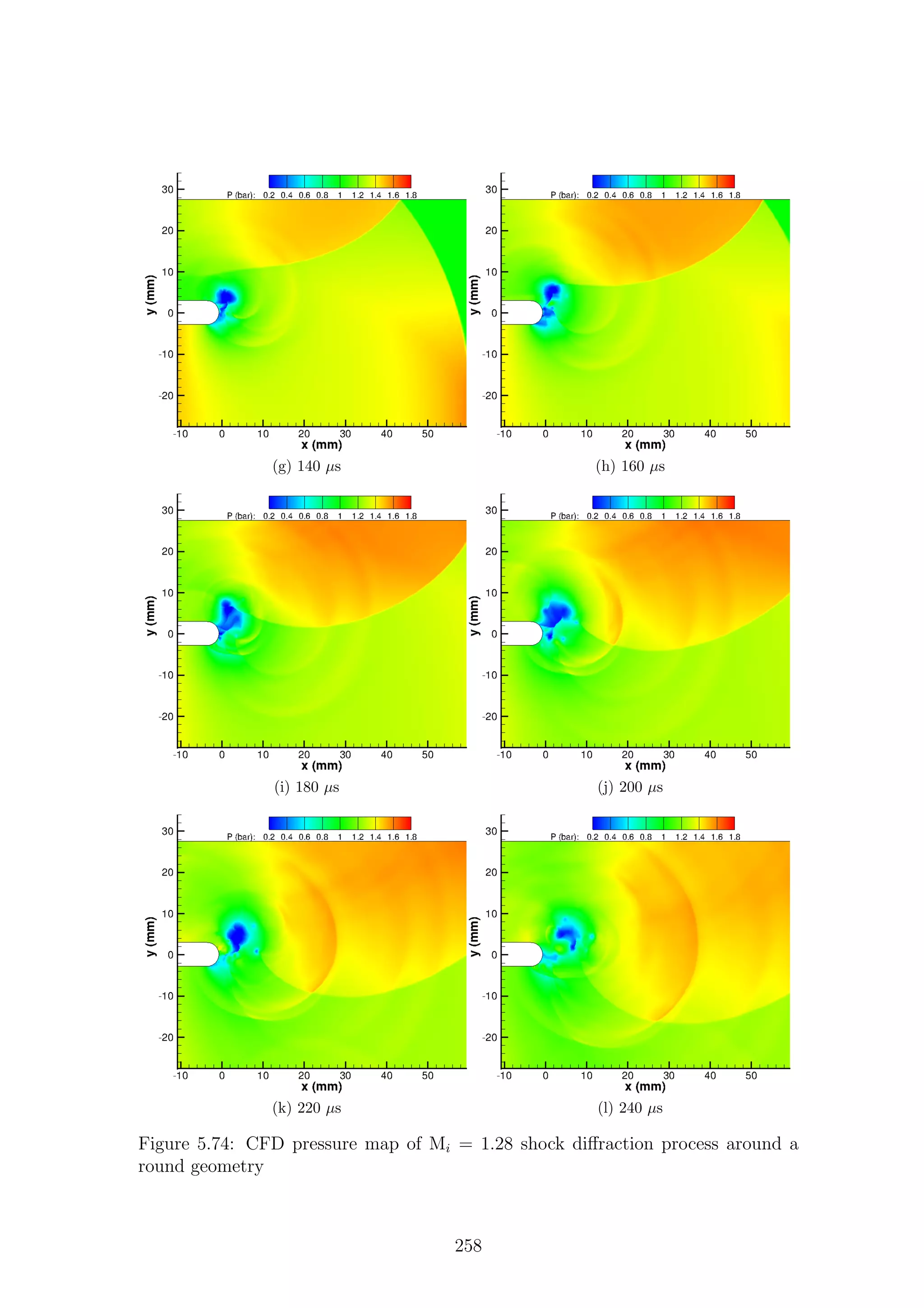
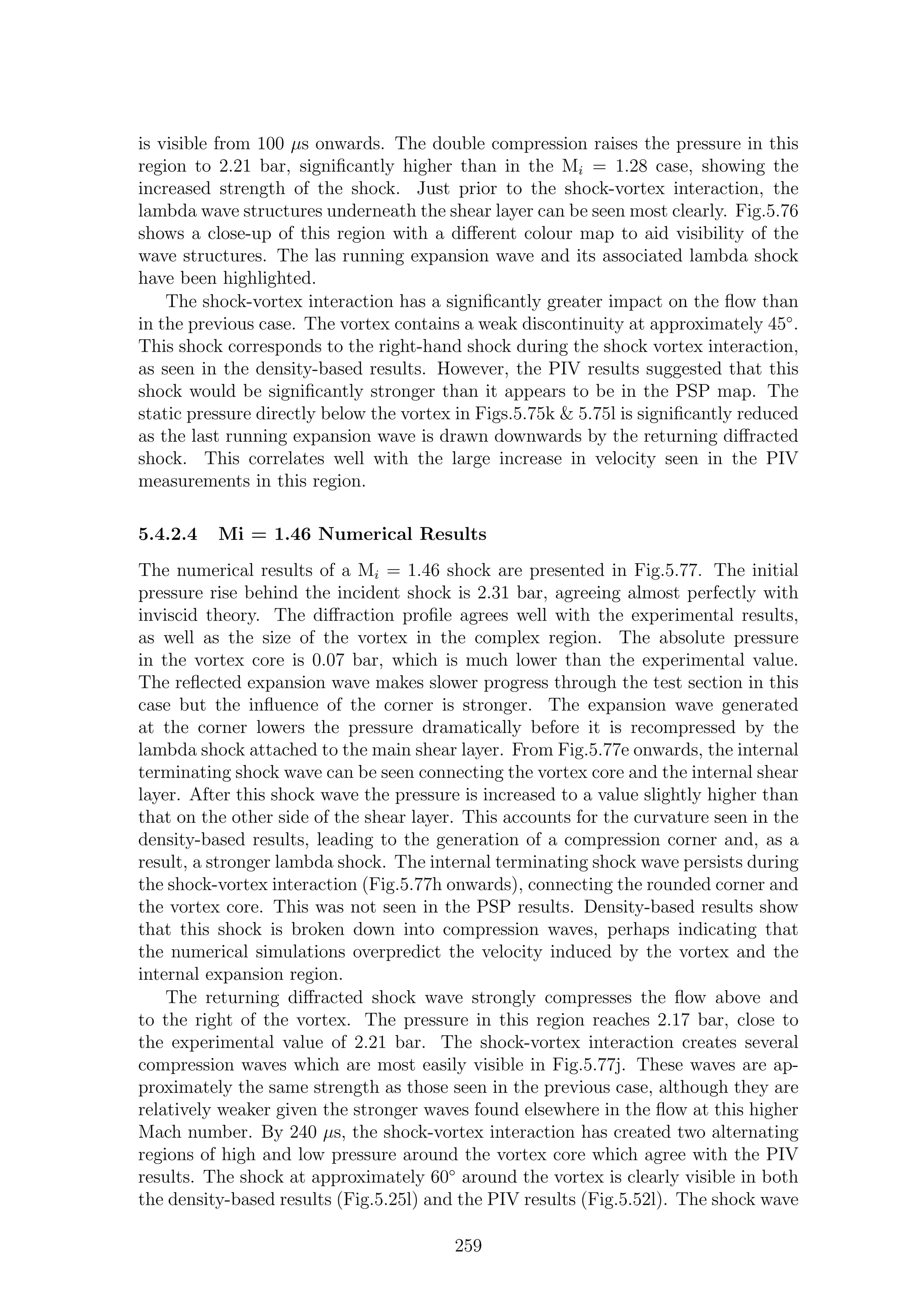
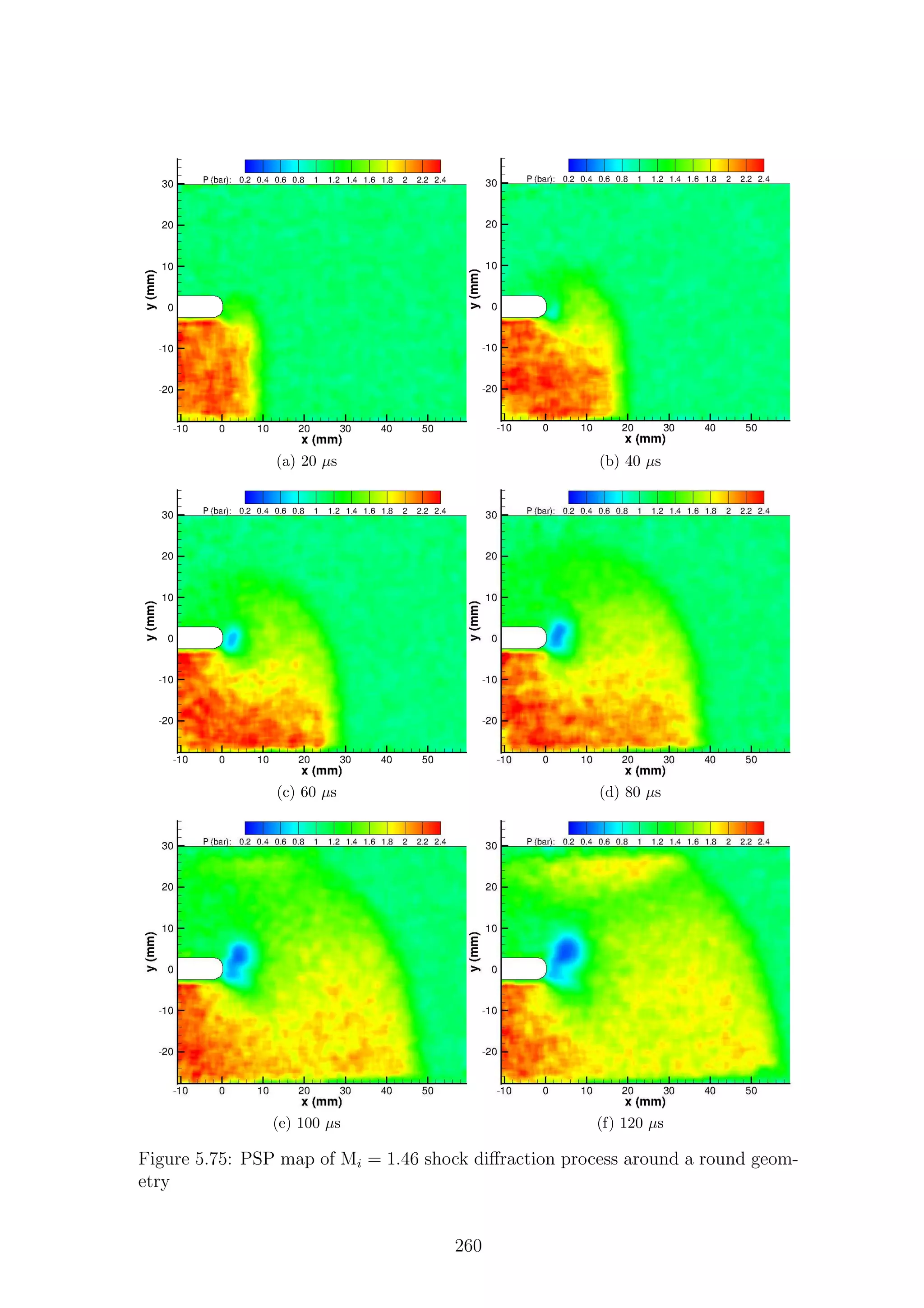
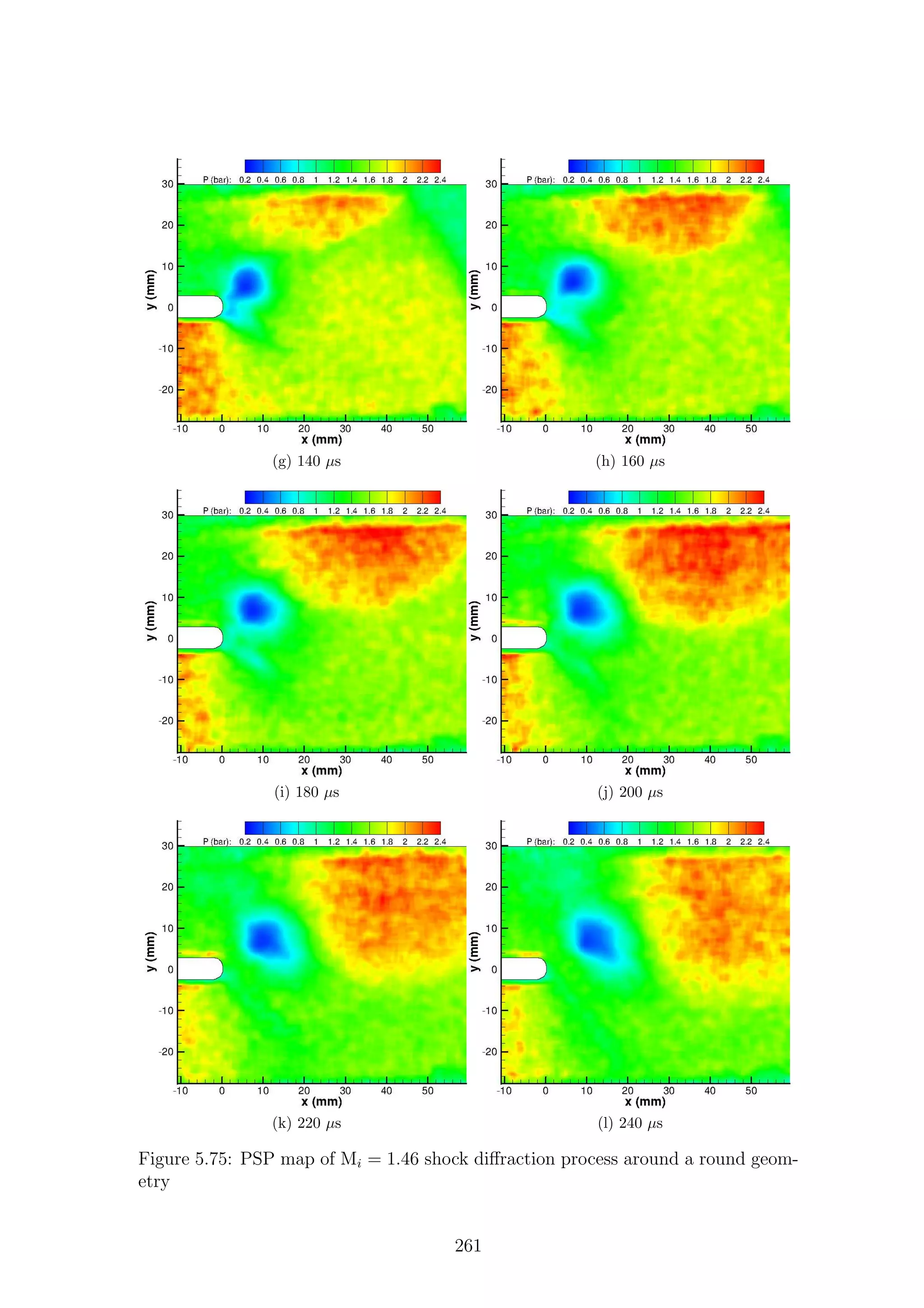
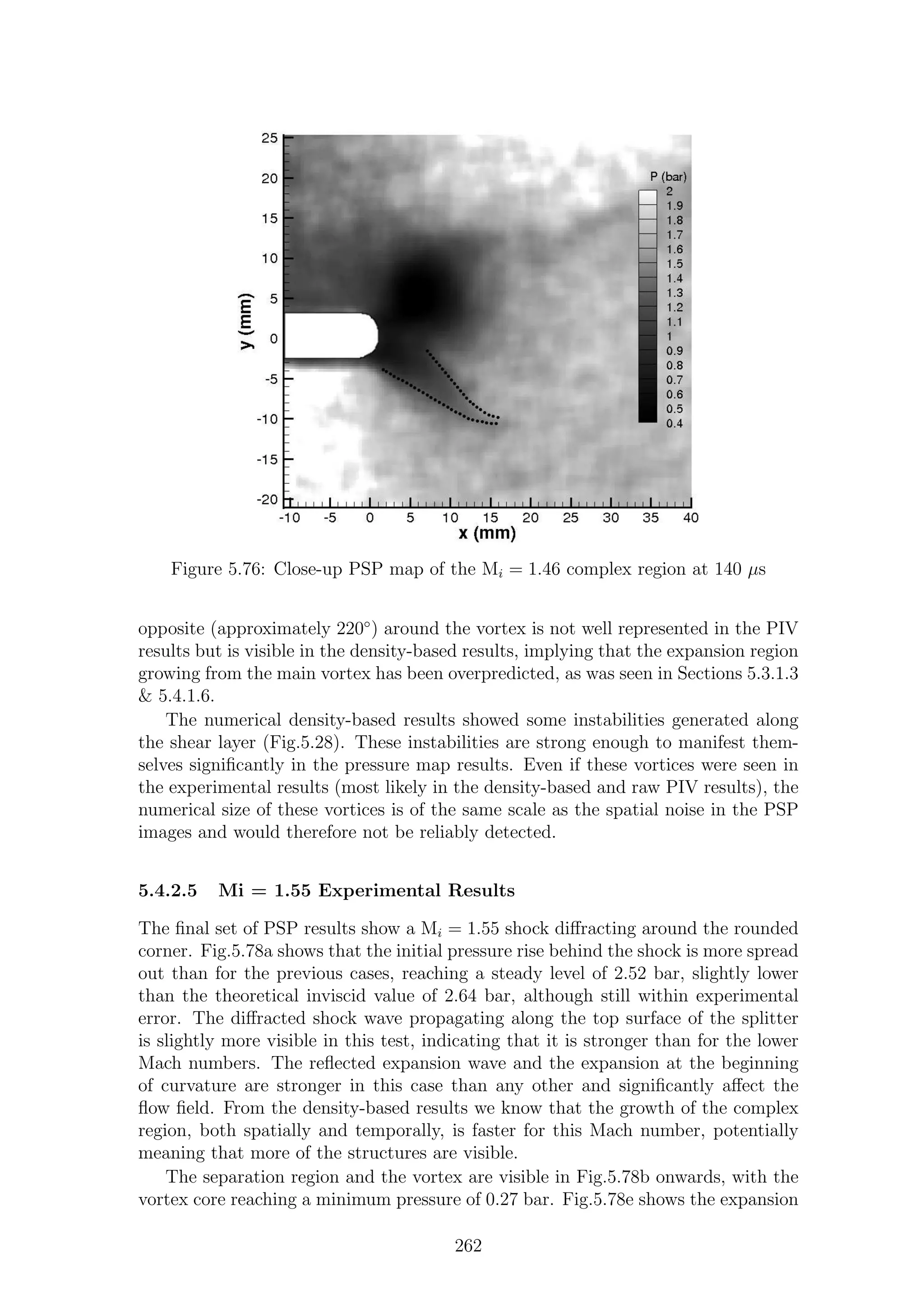
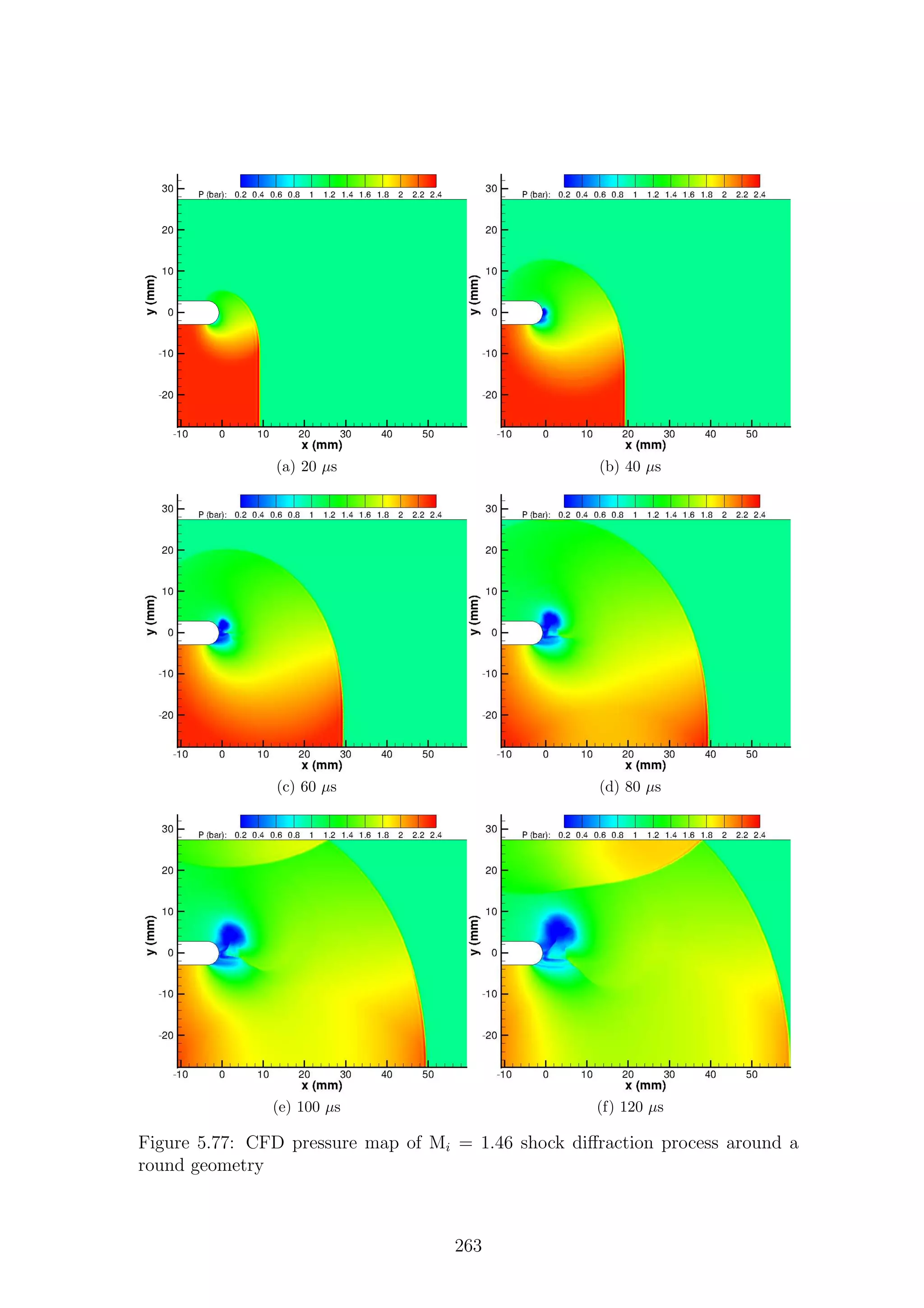

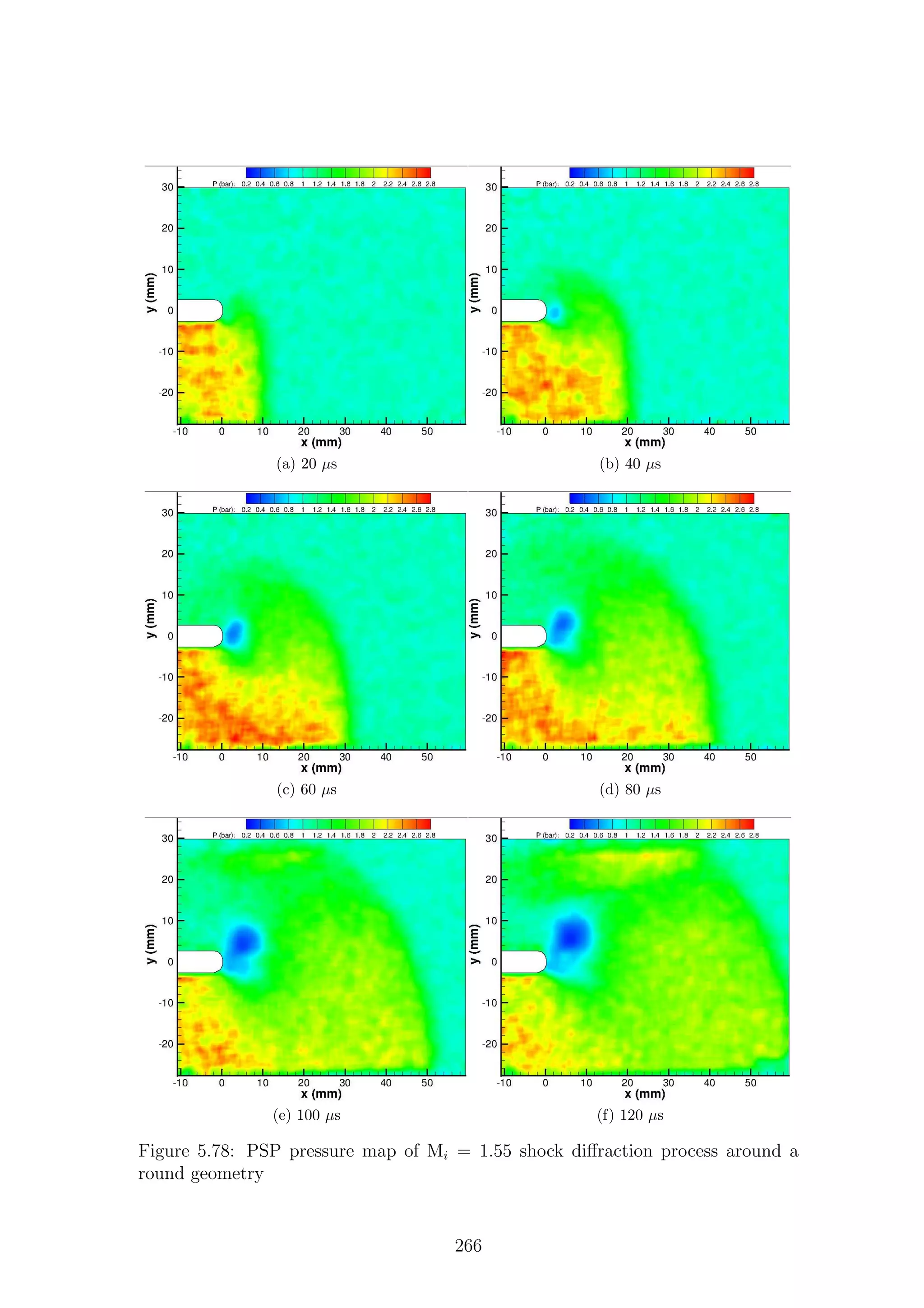
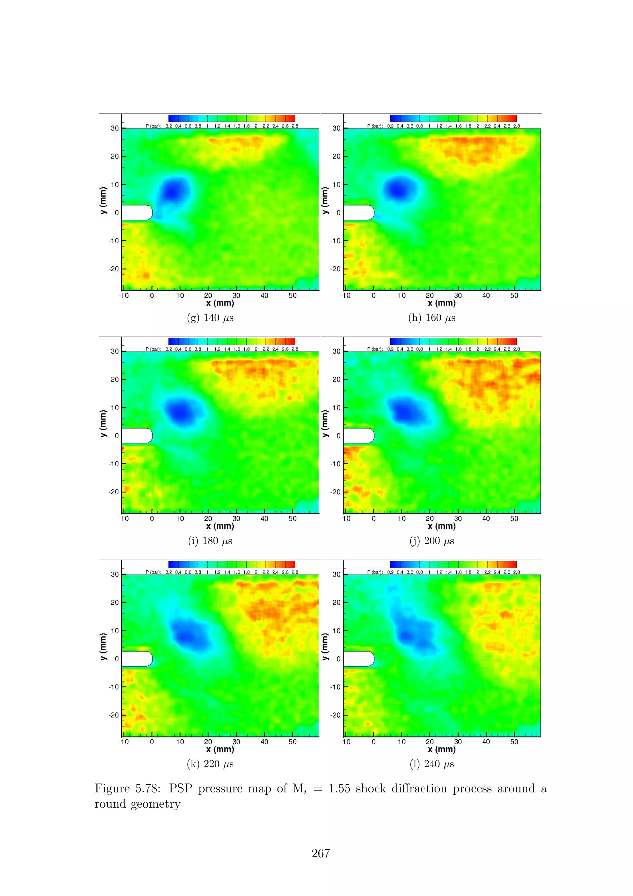
![Figure 5.79: Close-up PSP map of the Mi = 1.55 complex region at 140 µs
5.4.2.7 Conclusions
The conclusions presented in this section will not repeat conclusions already made
in Section 5.4.1.7 about the PSP technique and its limitations.
Pressure-sensitive paint has been applied to quantitatively measure the pressure
profile behind a shock wave diffracting around a rounded geometry. The complex
region behind a shock diffracting around a rounded corner is very difficult to mea-
sure, due to its slow spatial growth and given the already discussed spatial noise of
the high-speed TLC PSP technique used here.
Similarly to the sharp geometry, there is some disagreement between the experi-
mental and numerical results regarding the pressure in the vortex core. The pressure
in the vortex core is lower for the rounded geometry and the vortex is smaller in
size, especially for lower Mach numbers. However, initial shock wave profiles and
strengths agree well with the values from inviscid theory based on the experimental
Mach number measured from the density-based results, as do the values for the
secondary compression region caused by the diffracted shock reflecting off the top
wall.
The Mi = 1.55 case allows us to see some of the internal waves in the complex
region. The internal terminating shock wave can faintly be seen in the experimental
results and is easily visible in the numerical results.
It is interesting to note that the pressure in the expansion region under the main
shear layer is significantly lower than atmospheric (as was the case for the sharp
geometry). As the last running expansion wave has a larger turning angle (i.e. the
angle between horizontal and the main shear layer), the expansion is much stronger
than that of the sharp geometry; on a local level, this leads to much higher velocities
and stronger interactions. The theory of Sun & Takayama [36] predicts that, for the
Mi = 1.28 case, the pressure after the expansion wave must be 0.83 bar or lower for
268](https://image.slidesharecdn.com/4a6f74b5-6bbb-4ffd-b3f5-7486cdb057cd-150303082443-conversion-gate01/75/Mark-Quinn-Thesis-299-2048.jpg)
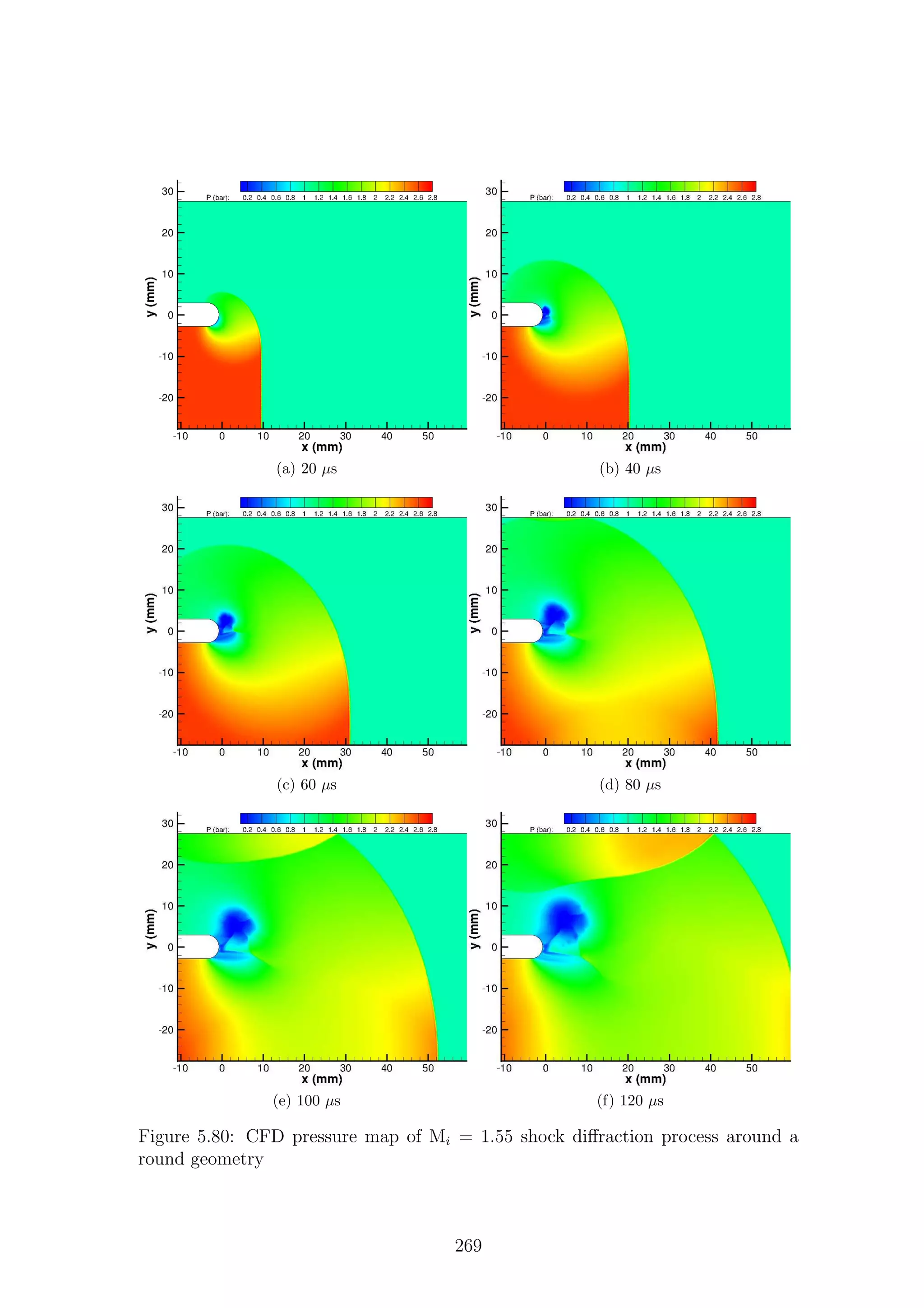
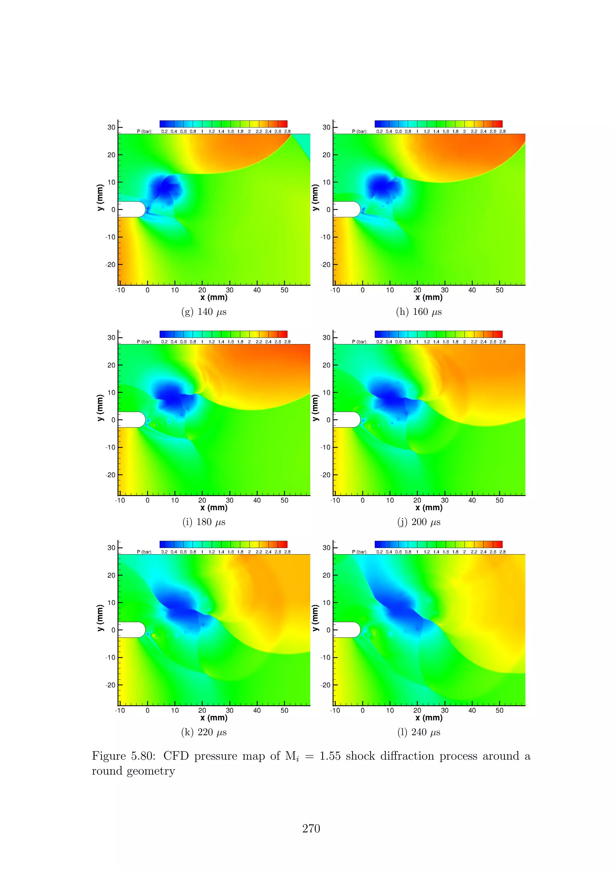


![7.2 Variation of Splitter Geometry
In order to ascertain the variation of flow parameters with apex angle, more inves-
tigations are needed with different corner geometries. Skews [32][34] has performed
numerous investigations on angles smaller than 90◦
; however, there is limited existing
work on angles greater than 90◦
. As we have shown, the flow can only be completely
understood by combining diagnostic techniques; therefore, the flow around different
sharp corner angles should be investigated using the combined approach presented
here.
The radius of the rounded corner appears to change the flow features by changing
the associated length scale [42][46]. The combined diagnostic approach should be
applied to different corner radii to investigate this effect. In order to do this, a
significantly larger shock tube test section would be needed to allow for the longer
development time.
Three-dimensional geometries have been briefly investigated during this project
(geometric details are given in Appendix A). Appendix B shows some of the density-
based results. Due to the three-dimensionality of the flow, two-dimensional PIV
measurements would not be suitable. Either a stereoscopic or volumetric approach
should be used. Further to this, numerical simulations of this flow would not be
possible using the version of Fluent available during this project, which was running
on a desktop PC and was limited to 450,000 cells.
7.3 Investigations of Shock Motion with Co-Flow
Density-based results were gathered on the diffraction process of shocks around the
two geometries presented so far (and the four mentioned above) with a subsonic and
supersonic co-flow. As these investigations were only possible using density-based
techniques (PSP is possible but was not performed due to time constraints of the
loaned equipment), they do not give a complete understanding of the flow. Despite
this, a portion of the preliminary results is presented in Appendix C.
7.4 Further Numerical Simulations
Numerical simulations performed in this project were limited by the computational
power and software available. This restricted the use of more modern turbulence
models and also limited the use of Reynolds stress models. Inviscid and laminar sim-
ulations performed well; however, these had a very strong grid dependency, which
required a very good understanding of the flow already to be able to tailor the numer-
ical viscosity to act as a damping function. Future work on the topic should consider
using a GPU enabled code, as the benefits of such high-performance computing can
be an increase in processing speed of up to 100 times.
7.5 PSP Chemical Composition Optimisation
Due to the scope of the experimental work performed during this project, it was
not possible to completely optimise the chemical composition of the PSP samples.
278](https://image.slidesharecdn.com/4a6f74b5-6bbb-4ffd-b3f5-7486cdb057cd-150303082443-conversion-gate01/75/Mark-Quinn-Thesis-309-2048.jpg)
![Ideally, a study similar to those performed by Sakaue et al. [185][196][170], where
each independent parameter such as solvent polarity or solution concentration is
varied across a wide range, would be conducted. This parametric variation could
allow for great increases in the PSP signal output and pressure sensitivity, and is
the logical extension of the paper published by the author in the Sensors Journal
[156].
Other luminophores were investigated during this project, namely PtTFPP (Plat-
inum tetrakis-pentafluorophenyl Porphyrin) and PBA (Pyrene Butyric Acid). The
luminescent lifetime of PtTFPP is too long to be of use in this research; however,
PBA has a lifetime of the order of nanoseconds. As this value represents the abso-
lute minimum response time, theoretically at least, PBA is capable of much faster
PSP measurements than the Ruthenium complex used. The disadvantage of PBA
is that its excitation wavelength is mid to high UV. Not only is this range of light
dangerous to work with, but it is also very difficult to find a light source with enough
power to give a meaningful signal. Filtering broadband light sources is not an op-
tion, as regular filters cannot withstand the light throughput; therefore, a UV solar
simulator, primarily used for biological applications, seems to be the only possible
option. However, these are prohibitively expensive and can be dangerous to operate.
Other possible alternatives include UV LED flash lamps, although these suffer from
cooling issues and are not always repeatable from flash to flash.
7.6 Pressure-/Temperature-Sensitive Velocimetry
The lifetime-based method uses the luminescent lifetime of the photo-active molecules
to calculate the surface pressure. The reduction of luminescent intensity after an
initial excitation follows an exponential decay, which is a function of the partial
pressure of oxygen (Fig.7.1). A simple derivation of the theory behind this is given
by Gregory et al. [143] and also by Lui & Sullivan [153]. A sample is exposed to
a known pressure and then excited by a short pulse of light, typically from a laser.
The emission from the excited sample decays at a certain rate, depending on the
pressure (and temperature) on the surface. The rate of this decay is directly related
to the pressure by the Stern-Volmer equation shown in Section 3.4.2.
Fig.7.1 shows a typical intensity decay rate for an excited luminophore. The
intensity is measured at various points during the decay in order to calculate the
decay rate. This is typically modelled by a single exponential, but can be modelled
by multiple exponentials [153].
The lifetime-based method has the advantages that it is insensitive to luminophore
and light non-uniformity and does not require a wind-off image. A possible appli-
cation of lifetime-based decay is a hybrid method of PSP and PIV, which will be
referred to as pressure-sensing velocimetry (PSV).
This method involves seeding atomised luminophores into the flow and using
them as the tracer particles for PIV measurements. The flow would be illuminated
as shown in Fig.3.18; however, the laser used would emit light in the absorption range
of the PSP spectra. The luminophore would then emit a certain amount of light
(dependent on the pressure at that point) and lifetime calculations can be made.
As the luminescent lifetime of most luminophores is extremely short (O 100ns s),
the flow would appear frozen in lifetime measurements. A second laser pulse would
279](https://image.slidesharecdn.com/4a6f74b5-6bbb-4ffd-b3f5-7486cdb057cd-150303082443-conversion-gate01/75/Mark-Quinn-Thesis-310-2048.jpg)
![Figure 7.1: Decay of intensity and camera gates
excite the flow again at time ∆T later so that PIV calculations can be made. This
concept has been tested with some success by Kimura et al. [201]. It was suggested
in this study that one of the largest sources of error in the PSP measurements was, as
usual, the temperature-induced effects. However, if a second luminophore could be
introduced into the tracer particle, as shown by Hradil et al. [180], the dual lifetime
method could allow for the measurement of pressure, temperature and velocity in
one single run. The combination of velocity and two independent thermodynamic
variables means that all of the flow parameters can be calculated.
The potential advantages of this technique are clear to see; however, the technical
difficulties associated with it are far from trivial. The selection of a carrier particle
for the luminophore(s) has conflicting requirements. The particle must be large
enough to carry a sufficient amount of luminophore to give a detectable signal while
still being small enough to follow the flow closely. The luminescent decay must be
fast enough to be considered stationary by the PIV measurements. Initial research
has been done in this area by Kimura et al. [202].
This hybrid method has been suggested by researchers Abe et al. [203], Song
et al. [204] and Kimura et al. [201], but has never been perfected or applied to an
actual flow. This is an interesting area of research and should be explored, as the
potential benefits could be revolutionary.
280](https://image.slidesharecdn.com/4a6f74b5-6bbb-4ffd-b3f5-7486cdb057cd-150303082443-conversion-gate01/75/Mark-Quinn-Thesis-311-2048.jpg)
![Bibliography
[1] J. W. Miles. On the disturbed motion of a plane vortex sheet. Journal of
Fluid Mechanics, 4(5):538–552, 1958.
[2] D. I. Pullin and A. E. Perry. Some flow visualization experiments on the
starting vortex. Journal of Fluid Mechanics, 97(02):239–255, 1980.
[3] J-P. Marat. Recherches physiques sur le feu. Jombert, Paris, 1780.
[4] Fluorophores.org Database of Fluorescent Dyes Properties and Applications.
[5] A. Price. The Spitfire Story. Jane’s Information Group Incorporated, 1982.
[6] F. Ma, J-Y. Choi, and V. Yang. Propulsive Performance of Airbreathing Pulse
Detonation Engines. Journal of Propulsion and Power, 22(6):1188–1203, 2006.
[7] I. I. Glass. Shock Waves & Man. University of Toronto Institute for Aerospace
Studies, Toronto, 1974.
[8] C. Chaussy and E. Schmiedt. Shock wave treatment for stones in the upper
urinary tract. The Urologic Clinics of North America, 10(4):743, 1983.
[9] N. Sultan-Bichat, J. Menard, G. Perceau, F. Staerman, P. Bernard, and
Z. Reguia. Treatment of calcinosis cutis by extracorporeal shock-wave
lithotripsy. Journal of the American Academy of Dermatology, 66(3):424–429,
2012.
[10] M. H. Anderson, B. P. Puranik, J. G. Oakley, P. W. Brooks, and R. Bonazza.
Shock tube investigation of hydrodynamic issues related to inertial confine-
ment fusion. Shock Waves, 10(5):377–387, 2000.
[11] Formula1.com. Virgin Racing reveal details of the VR-01.
[12] TotalF1.com. Virgin to rely on CFD again, 2010.
[13] J. Allen. Virgin moves shows Marussia’s statement of intent to move up the
grid, 2011.
[14] TotalF1.com. Virgin gives up on all-CFD approach to F1, 2011.
[15] J. K. Wright. Shock Tubes. Methuen’s Monographs On Physical Subjects.
Spottiswoode, London, 1961.
[16] J. D. Anderson. Modern Compressible Flow With Historical Perspective.
McGraw-Hill, 3 edition, 2004.
281](https://image.slidesharecdn.com/4a6f74b5-6bbb-4ffd-b3f5-7486cdb057cd-150303082443-conversion-gate01/75/Mark-Quinn-Thesis-312-2048.jpg)
![[17] S. C. Lin. Rate of Ionization Behind Shock Waves in Air. Planetary and Space
Science, 6:94–99, 1961.
[18] R. Mariani. Experimental Studies on Compressible Vortex Loops. PhD thesis,
Manchester, 2012.
[19] H. Zare-Behtash, N. Gongora-Orozco, and K. Kontis. Global Visualization
and Quantification of Compressible Vortex Loops. Journal of Visualization,
12(3):233–240, 2009.
[20] I. I. Glass, W. Martin, and G. N. Patterson. A Theoretical and Experimental
Study of The Shock Tube, 1953.
[21] G. Ben-Dor. Shock Wave Reflection Phenomena. Springer, New-York, 1991.
[22] G. Ben-Dor. A State-of-the-Knowledge Review on Pseudo-Steady Shock-Wave
Reflections and their Transition Criteria. Shock Waves, 15(3):277–294, 2006.
[23] B. W. Skews and J. T. Ashworth. The Physical Nature of Weak Shock Wave
Reflection. Journal of Fluid Mechanics, 542:105–114, 2005.
[24] T. V. Bazhenova, L. G. Gvozdeva, and M. A. Nettleton. Unsteady interactions
of shock waves. Progress in Aerospace Sciences, 21(0):249–331, 1984. doi:
10.1016/0376-0421(84)90007-1.
[25] G. B. Whitham. A New Approach to Problems of Shock Dynamics Part 1:
Two-Dimensional Problems. Journal of Fluid Mechanics, 2:145–171, 1957.
[26] G. B. Whitham. A new approach to problems of shock dynamics Part 2: Three-
dimensional problems. Journal of Fluid Mechanics, 5(03):369–386, 1959.
[27] Z. Han and X. Yin. Shock Dynamics. Kluwer Academic, Dordrecht, 1993.
[28] B. W. Skews. The Shape of a Diffracting Shock Wave. Journal of Fluid
Mechanics, 29(2):297–304, 1967.
[29] K. Oshima, K. Sugaya, M. Yamamoto, and T. Totoki. Diffraction of a Plane
Shock Wave Around a Corner. ISAS report, 30(2):51–82, 1965.
[30] J. Rosciszewski. Propagation of waves of finite amplitude along a duct of
non-uniform cross-section. Journal of Fluid Mechanics, 8(04):625–633, 1960.
[31] R. F. Chisnell. The motion of a shock wave in a channel, with applications to
cylindrical and spherical shock waves. Journal of Fluid Mechanics, 2(03):286–
298, 1957.
[32] B. W. Skews. The Perturbed Region Behind a Diffracting Shock Wave. Journal
of Fluid Mechanics, 29(4):705–719, 1967.
[33] B. W. Skews, C. Law, A. Muritala, and S. Bode. Shear layer behavior resulting
from shock wave diffraction. Experiments in Fluids, 52(2):417–424, 2012.
282](https://image.slidesharecdn.com/4a6f74b5-6bbb-4ffd-b3f5-7486cdb057cd-150303082443-conversion-gate01/75/Mark-Quinn-Thesis-313-2048.jpg)
![[34] B. W. Skews, C. Law, A. Muritala, and S. Bode. Shear Layer Evolution in
Shock Wave Diffraction. In K Kontis, editor, 28th International Symposium
on Shock Waves, Manchester, UK, 2011. Springer.
[35] T. V. Bazhenova, L. G. Gvozdeva, V. S. Komarov, and B. G. Sukhov. Diffrac-
tion of strong shock waves by convex corners. Fluid Dynamics, 8(4):611–619,
1973.
[36] M. Sun and K. Takayama. The Formation of a Secondary Wave Behind a
Shock Wave Diffracting at a Convex Corner. Shock Waves, 7:287–295, 1997.
[37] H. Kleine, E. Ritzerfeld, and H. Groenig. Shock wave diffraction: new aspects
on an old problem. In R Brun and L Z Dumitrescu, editors, 19th International
Symposium on Shock Waves, Marseille, France, 1995. Springer.
[38] R. Hillier. Computation of Shock Wave Diffraction at a Ninety Degrees Corner.
Shock Waves, 1:89–98, 1991.
[39] T. V. Bazhenova, S. B. Bazarov, O. V. Bulat, V. V. Golub, and A. M.
Schul’meister. Experimental and numerical study of shock wave attenuation
at the outlet of two-dimensional and axisymmetric ducts. Fluid Dynamics,
28(4):590–593, 1993.
[40] S-M. Chang, K-S. Chang, and S. Lee. Reflection and Penetration
of a Shock Wave Interacting with a Starting Vortex. 42(4):796–805,
2004. Korea Advanced Institute of Science and Technology (KAIST)
[http://koasas.kaist.ac.kr/dspace-oai/request] (Korea, Republic of) ER.
[41] N. Gongora-Orozco, H. Zare-Behtash, K. Kontis, and C. Hale. Particle Image
Velocimetry Studies on Shock Wave Diffraction with Co-Flow Jet. In K C Kim
and S J Lee, editors, 14th International Symposium on Flow Visualization,
Daegu, Korea, 2010.
[42] B. W. Skews. Shock Diffraction on Rounded Corners. In Thrid Australasian
conference on Hydraulics and Fluid Mechanics, Sydney, Australia, 1968.
[43] Y. P. Lagutov. Shape of a shock wave diffracted by a rounded corner. Fluid
Dynamics, 18(3):484–487, 1983.
[44] C. Law, S. Menon, and B. W. Skews. Near-wall features in transient com-
pressible flow on convex walls. In G Jagadeesh, editor, 25th International
Symposium on Shock Waves, Bangalore, India, 2005.
[45] M. Sun and K. Takayama. Vorticity Production in Shock Diffraction. Journal
of Fluid Mechanics, 478:237–256, 2003.
[46] A. Muritala, C. Law, and B. W. Skews. Shock wave diffraction on convex
curved walls. In K Kontis, editor, 28th International Symposium on Shock
Waves, Manchester, UK, 2011. Springer.
283](https://image.slidesharecdn.com/4a6f74b5-6bbb-4ffd-b3f5-7486cdb057cd-150303082443-conversion-gate01/75/Mark-Quinn-Thesis-314-2048.jpg)
![[47] H. Hasegawa, M. Fujimoto, T-D. Phan, H. Reme, A. Balogh, M. W. Dunlop,
C. Hashimoto, and R. TanDokoro. Transport of solar wind into Earth’s mag-
netosphere through rolled-up Kelvin-Helmholtz vortices. Nature, 430:755–758,
2004.
[48] P. G. Drazin and W. H. Reid. Hydrodynamic Stability. Cambridge Monographs
on Mechanics. Cambridge University Press, Cambridge, 1982.
[49] R. Betchov and Criminale W. O. Stability of Parallel Flows. Academic Press,
New York, 1967.
[50] E. M. Greitzer, C. S. Tan, and M. B. Graf. Internal Flow: Concepts and
Applications. Cambridge University Press, New York, 2004.
[51] R. F. Davey and A. Roshko. The effect of density difference on shear-layer
instability. Journal of Fluid Mechanics, 53(3):523–543, 1972.
[52] D. Papamoschou and A. Roshko. The Compressible Turbulent Shear Layer:
An Experimental Study. Journal of Fluid Mechanics, 197:453–477, 1988.
[53] P. A. Monkewitz and P. Huerre. Influence of the velocity ratio on the spatial
instability of mixing layers. Physics of Fluids, 25(7):1137–1143, 1982.
[54] J. Abraham and V. Magi. Exploring Velocity and Density Ratio Effects in
a Mixing Layer Using DNS. International Journal of Computational Fluid
Dynamics, 8(2):147–151, 1997. doi: 10.1080/10618569708940801.
[55] Lord Rayleigh. On the Dynamics of Revolving Fluids. Proceedings of the
Royal Society of London. Series A, Containing Papers of a Mathematical and
Physical Character, 93(648):148–154, 1880.
[56] G. L. Brown and A. Roshko. On Density Effects and Large Structure in Turbu-
lent Mixing Layers. Journal of Fluid Mechanics Digital Archive, 64(04):775–
816, 1974.
[57] A. Roshko. Structure of Turbulent Shear Flows: A New Look. AIAA Journal,
14(10):1349–1357, 1976.
[58] D. W. Bogdanoff. Compressibility Effects in Turbulent Shear layers. AIAA
Journal, 21(6):926–927, 1983.
[59] G. S. Elliott and M. Samimy. Compressibility Effects in Free Shear Layers.
Physics of Fluids, 2(7):1231–1240, 1990.
[60] W. W. Liou. Linear instability of curved free shear layers. Physics of Fluids,
6(2):541–549, 1993.
[61] L. Prandtl and O. G. Tietjens. Applied hydro-and aeromechanics, volume 2.
Dover publications, 1957.
[62] Q. Lian and Z. Huang. Starting flow and structures of the starting vortex
behind bluff bodies with sharp edges. Experiments in Fluids, 8(1):95–103,
1989.
284](https://image.slidesharecdn.com/4a6f74b5-6bbb-4ffd-b3f5-7486cdb057cd-150303082443-conversion-gate01/75/Mark-Quinn-Thesis-315-2048.jpg)
![[63] D. W. Moore. A numerical study of the roll-up of a finite vortex sheet. Journal
of Fluid Mechanics, 63(02):225–235, 1974.
[64] H. Kaden. Aufwicklung einer unstabilen Unstetigkeitsflache. PhD thesis, 1931.
[65] D. S. Dosanjh and T. M. Weeks. Interaction of a Starting Vortex as Well as
a Vortex Street with a Travelling Shock Wave. AIAA Journal, 3(2):216–223,
1965.
[66] J. L. Ellzey, M. R. Henneke, J. M. Picone, and E. S. Oran. The Interaction
of a Shock with a Vortex: Shock Distortion and the Production of Acoustic
Waves. Physics of Fluids, 7(1):172–184, 1995.
[67] F. Grasso and S. Pirozzoli. Shock-Wave-Vortex Interactions: Shock and Vortex
Deformations, and Sound Production. Theoretical and Computational Fluid
Dynamics, 13:421–456, 2000.
[68] K-S. Chang and S-M. Chang. Scattering of Shock into Acoustic Waves in
Shock-Vortex Interaction. Materials Science Forum, pages 131–138, 2004.
[69] K-S. Chang, H. Barik, and S-M. Chang. The Shock-Vortex Interaction Pat-
terns Affected by Vortex Flow Regime and Vortex Models. Shock Waves,
19:349–360, 2009.
[70] A. Chatterjee and S. Vijayaraj. Multiple Sound Generation in Interaction of
Shock Wave with Strong Vortex. AIAA Journal, 46(10):2558–2567, 2008.
[71] B. W. Skews. Curved shock wave interaction with a spiral vortex. In Z Jiang,
editor, 24th International Symposium on Shock Waves, volume 2, pages 1317–
1322, Beijing, China, 2004. Springer.
[72] S-M. Chang and K-S. Chang. Successive Interactions of a Shock Wave with
Serially Arranged Vortices. KSME International Journal, 18(4):664–670, 2004.
[73] F. J. Barbosa and B. W. Skews. Shock wave interaction with a spiral vortex.
Physics of Fluids, 13(10):3049–3060, 2001.
[74] B. Strurtevant and V. A. Kulkarny. The focusing of weak shock waves. Journal
of Fluid Mechanics, 73(4):651–671, 1976.
[75] G. A. Sod. A survey of several finite difference methods for systems of nonlinear
hyperbolic conservation laws. Journal of Computational Physics, 27(1):1–31,
1978. doi: 10.1016/0021-9991(78)90023-2.
[76] K. Takayama and Y. Inoue. Shock Wave Diffraction over a 90 degree Sharp
Corner. Shock Waves, 1:301–312, 1991.
[77] J. H. Ferziger and M. Peric. Computation Methods for Fluid Dynamics.
Springer, Berlin, 3rd edition, 2002.
[78] M. Sun and K. Takayama. A Note on Numerical Simulation of Vortical Struc-
tures in Shock Diffraction. Shock Waves, 13:25–32, 2003.
285](https://image.slidesharecdn.com/4a6f74b5-6bbb-4ffd-b3f5-7486cdb057cd-150303082443-conversion-gate01/75/Mark-Quinn-Thesis-316-2048.jpg)
![[79] G. Abate and W. Shyy. Dynamic Structure of Confined Shocks Undergoing
Sudden Expansion. Progress in Aerospaces Sciences, 38, 2002.
[80] S. M. Liang, W. T. Chung, H. Chen, and S-H. Shyu. Numerical Investigation
of Reflected Shock Vortex Interaction Near an Open Ended Duct. AIAA
Journal, 43(2):349–356, 2005.
[81] T. I. Tseng and R. J. Yang. Numerical Simulation of Vorticity Production in
Shock Diffraction. AIAA Journal, 44(5):1040–1047, 2006.
[82] S. De and M. Thangadurai. Numerical Simulation of Shock Tube Generated
Vortex Effect of Numerics. International Journal of Computational Fluid Dy-
namics, 25(6):345–354, 2011.
[83] N. Uchiyama and O. Inoue. Shock Wave/ Vortex Interaction in a Flow over a
90-deg Sharp Corner. AIAA Journal, 33(9):1740–1743, 1995.
[84] Z. Jiang, K. Takayama, H. Babinsky, and T. Meguro. Transient Shock Wave
Flows in Tube with Sudden Change in Cross Section. Shock Waves, 7, 1997.
[85] K. D. Jensen. Flow Measurements. Journal of the Brazilian Society of Me-
chanical Sciences and Engineering, 26:400–419, 2004.
[86] H. Kleine, H. Groenig, and K. Takayama. Simultaneous Shadow, Schlieren
and Interferometric Visualization of Compressible Flows. Optics and Lasers
in Engineering, 44:170–189, 2006.
[87] J. Rienitz. Optical inhomogeneities: schlieren and shadowgraph methods in
the seventeenth and eighteenth centuries. Endeavour, 21(2):77–81, 1997.
[88] R. Hooke. Micrographia: or some Physiological Descriptions of Minute Bodies
made by Magnifying Glasses with Observations and Inquiries thereupon. 1667.
[89] T. Birch. The history of the Royal Society of London for improving of natural
knowledge from its first rise, in which the most considerable of those papers
communicated to the Society, which have hitherto not been published, are in-
serted as a supplement to the Philosophical Transactions, volume 3. Printed
for A. Millar in the Strand, London, 1757. v. 3.
[90] M. Burgan. Robert Hooke: Natural Philosopher and Scientific Explorer. Com-
pass Point Books, 2008.
[91] J. Rienitz. Schlieren experiment 300 years ago. Nature, 254:293–295, 1975.
[92] P. Heering. Public Experiments and their Analysis with the Replication
Method. Science & Education, 2006.
[93] O. Reynolds. An Experimental Investigation of the Circumstances which de-
termine whether the Motion of Water shall be Direct or Sinuous, and the Law
of Resistance in Parallel Channels. Philosophical Transactions of the Royal
Society, 174:935–982, 1883.
[94] J. Darius. Visions of sound. New Scientist, 16 May 1974 1974.
286](https://image.slidesharecdn.com/4a6f74b5-6bbb-4ffd-b3f5-7486cdb057cd-150303082443-conversion-gate01/75/Mark-Quinn-Thesis-317-2048.jpg)
![[95] L. Foucault. Memoire sur la construction des telescopes en verre argente.
Annales de l’Observatoire de Paris, 5:197–237, 1859.
[96] P. Krehl and S. Engemann. August Toepler - the first who visualized shock
waves. Shock Waves, 5:1–18, 1995.
[97] A. J. I. Toepler and A. Witting. Beobachtungen nach einer neuen optischen
methode: Ein beitrag experimentalphysik. W. Engelmann, 1906.
[98] H. G. Taylor and J. M. Waldram. Improvements in the Schlieren method.
Journal of Scientific Instruments, 10(12):378–389, 1933.
[99] T. Smith. Foucault or Toepler? Journal of Scientific Instruments, 11(32):32–
33, 1934.
[100] H. Kleine and G. S. Settles. The art of shock waves and their flowfields. Shock
Waves, 17:291–307, 2008.
[101] H. Kleine. Filming the invisible - time-resolved visualization of compressible
flows. The European Physical Journal Special Topics, 180:3–34, 2010.
[102] G. E. A. Meier. Hintergrund Schlierenverfahren, 1999.
[103] M. Raffel, H. Richard, and G. E. A. Meier. On the applicability of background
oriented optical tomography for large scale aerodynamic investigations. Ex-
periments in Fluids, 28:477–481, 2000.
[104] G. E. A. Meier. Computerized background-oriented schlieren. Experiments in
Fluids, 33:181–187, 2002.
[105] F. Leopold, D. Klatt, F. Jagusinski, and C. Demeautis. Error estimation
for the colored background oriented schlieren techniques (CBOS). In 8th Pa-
cific Symposium on flow Visualization and Image Processing, Moscow, Russia,
2011.
[106] D. Papamoschou. A Two-Spark Schlieren System for Very-High Velocity Mea-
surements. Experiments in Fluids, 7:354–356, 1989.
[107] G. S. Settles. Schlieren and Shadowgraph Techniques. Experimental fluid
Mechanics. Springer, Berlin, 2001.
[108] W. Merzkirch. Flow Visualization. Academic Press Inc., Florida, second
edition, 1987.
[109] M. M. Biss, G. S. Settles, M. J. Hargather, L. J. Dodson, and J. D. Miller.
High-speed digital shadowgraphy of shock waves from explosions and gun-
shots. In Klaus Hannemann and Friedrich Seiler, editors, 26th International
Symposium on Shock Waves, Gottingen, Germany, 2007.
[110] R. J. Goldstein. Fluid Mechanics Measurements. Taylor & Francis, Washing-
ton DC, 2nd edition, 1996.
287](https://image.slidesharecdn.com/4a6f74b5-6bbb-4ffd-b3f5-7486cdb057cd-150303082443-conversion-gate01/75/Mark-Quinn-Thesis-318-2048.jpg)
![[111] G. S. Speak and D. J. Walters. Optical Considerations and Limitations of the
Schlieren Method. Technical report, Aeronautical Research Council, 1954.
[112] C. M. Vest. Holographic Interferometry. John Wiley & Sons, New York, 1979.
[113] T. Kreis. Handbook of Holographic Interferometry - Optical and Digital Meth-
ods. Wiley-VCH, Weinheim, 2005.
[114] M. J. Hargather, G. S. Settles, and M. J. Madalis. Schlieren imaging of loud
sounds and weak shock waves in air near the limit of visibility. Shock Waves,
20:9–17, 2010.
[115] H. Kleine and H. Groenig. Color schlieren methods in shock wave research.
Shock Waves, 1:51–63, 1991.
[116] W. L. Howes. Rainbow schlieren and its applications. Applied Optics,
23(14):2449–2460, 1984.
[117] D. Pierce. Photographic evidence of the formation and growth of vorticity
behind plates accelerated from rest in still air. Journal of Fluid Mechanics,
11(03):460–464, 1961.
[118] A. R. Greenleaf. Photographic Optics. The MacMillan Company, New York,
1950.
[119] L. Prandtl. Uber Flussigkeitsbewegung Bei Sehr Kleiner Reibung. In verh iii
Int. math. Kongr., Heidelberg, pages 484–491, 1905.
[120] R. J. Adrian. Twenty years of particle image velocimetry. Experiments in
Fluids, 39:159–169, 2005.
[121] G. E. Elsinga, B. Wieneke, F. Scarano, and A. Schroeder. Tomographic 3D-
PIV and Applications. In A Schroeder and C E Willert, editors, Particle Image
Velocimetry: New Developments and Recent Applications. Springer, Berlin,
2008.
[122] F. F. J. Schrijer, F. Scarano, and B. W. van Oudheusden. Application of PIV
in a Mach 7 Double-Ramp Flow. Experiments in Fluids, 41:353–363, 2006.
[123] R. Theunissen, F. Scarano, and M. L. Tiethmuller. An Adaptive Sampling and
Windowing Interrogation Method in PIV. Measurement Science and Technol-
ogy, 18:275–287, 2007.
[124] M. Havermann, J. Haertig, C. Rey, and A. George. PIV Measurements in
Shock Tunnels and Shock Tubes. In A Schroeder and C E Willert, edi-
tors, Particle Image Velocimetry: New Developments and Recent Applications.
Springer, 2008.
[125] M. J. Molezzi and J. C. Dutton. Application of Particle Image Velocimetry in
high-Speed Separated Flows. AIAA Journal, 31(3):439–446, 1993.
[126] M. Raffel, C. E. Willert, S. T. Wereley, and J. Kompenhans. Particle Image
Velocimetry: A Practical Guide. Springer, Berlin, 2007.
288](https://image.slidesharecdn.com/4a6f74b5-6bbb-4ffd-b3f5-7486cdb057cd-150303082443-conversion-gate01/75/Mark-Quinn-Thesis-319-2048.jpg)
![[127] H. Ounis, G. Ahmadi, and J. B. McLaughlin. Brownian diffusion of submi-
crometer particles in the viscous sublayer. Journal of Colloid and Interface
Science, 143(1):266–277, 1991. doi: 10.1016/0021-9797(91)90458-K.
[128] S. G. Jennings. The mean free path in air. Journal of Aerosol Science,
19(2):159–166, 1988. doi: 10.1016/0021-8502(88)90219-4.
[129] A. Melling. Tracer Particles and Seeding for Particle Image Velocimetry. Mea-
surement Science and Technology, 8:1406–1416, 1997.
[130] M. Samimy and S. K. Lele. Motion of Particles with Inertia in a Compressible
Free Shear Layer. Physics of Fluids, 3(8), 1991.
[131] D. Ragni, F. Schrijer, B. van Oudheusden, and F. Scarano. Particle tracer
response across shocks measured by PIV. Experiments in Fluids, 50(1):53–64,
2011.
[132] S. Ghaemi, A. Schmidt-Ott, and F. Scarano. Nanostructured tracers for laser-
based diagnostics in high-speed flows. Measurement Science and Technology,
21(10):105403, 2010.
[133] F. Scarano. Overview of PIV in Supersonic Flows. In A Schroeder and C E
Willert, editors, Particle Image Velocimetry: New Developments and Recent
Applications. Springer, 2008.
[134] C. Hale, R. Efrani, and K. Kontis. Plasma Actuators with Multiple Encapsu-
lated Electrodes to Influence the Induced Velocity. In 48th AIAA Aerospace
Sciences Meeting, Orlando, Florida, 2010. AIAA.
[135] C. Hale, R. Efrani, and K. Kontis. Plasma Actuators with Multiple Encapsu-
lated Electrodes to Influence the Induced Velocity: Further Configurations. In
40th AIAA Fluid Dynamics Conference and Exhibit, Chicago, Illinois, 2010.
AIAA.
[136] D. Ragni, A. Ashok, B. W. van Oudheusden, and F. Scarano. Surface Pres-
sure and Aerodynamic Loads Determination of a Transonic Airfoil Based on
Particle Image Velocimetry. Measurement Science and Technology, 20, 2009.
[137] J. Haertig, M. Havermann, C. Rey, and A. George. Particle Image Velocimetry
in Mach 3.5 and 4.5 Shock-Tunnel Flows. AIAA Journal, 40(6):1056–1060,
2002.
[138] F. F. J. Schrijer, R. Caljouw, F. Scarano, and B. W. van Oudheusden. Three
Dimensional Experimental Investigation of a Hypersonic Double-Ramp Flow.
In A. Schroeder and C. E. Willert, editors, Particle Image Velocimetry: New
Developments and Recent Applications, pages 719–724. Springer, 2008.
[139] R. A. Humble, F. Scarano, and B. W. van Oudheusden. Particle Image Ve-
locimetry Measurements of a Shock Wave/Turbulent Coundary Layer Inter-
action. Experiments in Fluids, 43:173–183, 2007.
289](https://image.slidesharecdn.com/4a6f74b5-6bbb-4ffd-b3f5-7486cdb057cd-150303082443-conversion-gate01/75/Mark-Quinn-Thesis-320-2048.jpg)
![[140] R. A. Humble, G. E. Elsinga, F. Scarano, and B. W. van Oudheusden. Investi-
gation of the Instantaneous 3D Flow Organization of a Shock Wave/Turbulent
Bouldanr Layer Interaction using Tomographic PIV. In 37th AIAA Fluid Dy-
namics Conference and Exhibit, Miami, Florida, 2007. AIAA.
[141] various. Particle Image Velocimetry. In C. Tropea, A. Yarin, and J. F. Foss,
editors, Springer Handbook of Experimental Fluid Dynamics, pages 309–342.
Springer, Berlin, 2007.
[142] G. E. Elsinga, B. W. van Oudheusden, and F. Scarano. Evaluation of Aero-
Optical Distortion Effects in PIV. Experiments in Fluids, 39, 2005.
[143] J. W. Gregory, K. Asai, M. Kameda, T. Lui, and J. P. Sullivan. A Review of
Pressure-Sensitive Paint for High Speed and Unsteady Aerodynamics. Proceed-
ings of the Institution of Mechanical Engineers, Part G: Journal of Aerospace
Engineering, 222(2):249–290, 2008.
[144] O. Stern and M. Volmer. On the quenching-time of fluorescence. Physik
Zeitschr, 20:183–188, 1919.
[145] H. Kautsky and H. Hirsch. Detection of minutest amounts of oxygen by ex-
tinction of phosphorescence. Z. Anorg. Allg. Chem, 222:126, 1935.
[146] J. P. Crowder. Fluorescent Minitufts. In W-J. Yang, editor, Handbook of Flow
Visualization. Taylor-Francis, 1989.
[147] B. G. McLachlan, J. L. Kavandi, J. B. Callis, M. Gouterman, E. Green,
G. Khalil, and D. Burns. Surface Pressure Mapping Using Luminescent Coat-
ings. Experiments in Fluids, 14:33–41, 1993.
[148] J. L. Kavandi, J. B. Callis, M. Gouterman, G. Khalil, D. Wright, E. Green,
D. Burns, and B. G. McLachlan. Luminescent barometry in wind tunnels.
Review of Scientific Instruments, 61(11):3340–3347, 1990.
[149] I. A. Zakharov, V. B. Aleskovsky, and T. I. Grishaeva. Phosphorescence of
trypaflavin on silica and its quenching by oxygen. Journal of Applied Spec-
troscopy, 1964.
[150] M. M. Ardasheva, L. B. Nevskii, and G. E. Pervushin. Measurement of pres-
sure distribution by means of indicator coatings. Journal of Applied Mechanics
and Technical Physics, 26(4):469–474, 1985.
[151] C. M. McGraw, J. H. Bell, G. Khalil, and J. B. Callis. Dynamic Surface
Pressure Measurements on a Square Cylinder with Pressure Sensitive Paint.
Experiments in Fluids, 40:203–211, 2005.
[152] J. W. Gregory, H. Sakaue, J. P. Sullivan, and S. Raghu. Characterization
of miniature fluidic oscillator flowfields using porous pressure sensitive paint.
In ASME Fluids Engineering Division Summer Meeting, New Orleans, USA,
2001.
290](https://image.slidesharecdn.com/4a6f74b5-6bbb-4ffd-b3f5-7486cdb057cd-150303082443-conversion-gate01/75/Mark-Quinn-Thesis-321-2048.jpg)
![[153] T. Liu and J. P. Sullivan. Pressure and Temperature Sensitive Paints. Springer-
Verlag, Berlin, 2005.
[154] J. H. Bell, E. T. Schairer, L. A. Hand, and R. D. Mehta. Surface Pressure Mea-
surements Using Luminescent Coatings. Annual Review of Fluid Mechanics,
33:155–206, 2001.
[155] H. Sakaue. Anodized Aluminum Pressure Sensitive Paint for Unsteady Aero-
dynamic Applications. PhD thesis, Purdue University, 2003.
[156] M. K. Quinn, L. Yang, and K. Kontis. Pressure-Sensitive Paint: Effect of
Substrate. Sensors, 11(12):11649–11663, 2011.
[157] H. Zare-Behtash. Experimental Studies on Compressible Vortical Flows, Phe-
nomena and Interactions. PhD thesis, University of Manchester, 2009.
[158] B. J. Basu. Optical Oxygen Sensing Based on Luminescence Quenching of
Platinum Porphyrin Dyes Doped in Ormosil Coatings. Sensors and Actuators
B, 123:568/577, 2007.
[159] B. D. MacCraith and C. McDonagh. Enhanced Fluorescence Sensing Using
Sol-Gel Materials. Journal of Fluorescence, 12(3/4):333–342, 2002.
[160] A. E. Baron, J. D. Danielson, M. Gouterman, J. R. Wan, J. B. Callis, and
M. Blair. Submillisecond Response Times of Oxygen-Quenched Luminescent
Coatings. Review of Scientific Instruments, 64(12):3394–3402, 1993.
[161] Y. Sakamura, M. Mamtsumoto, and T. Suzuki. High Frame-Rate Imaging of
Surface Pressure Distribution Using a Porous Pressure-Sensitive Paint. Mea-
surement Science and Technology, 16:759–765, 2005.
[162] N. Gongora-Orozco. Experimental Studies on Internal Shock Wave Phe-
nomenon and Interactions. PhD thesis, University of Manchester, 2010.
[163] V. E. Mosharov, V. Radchenko, and S. Fonov. Luminescent Pressure Sen-
sors in Aerodynamic Experiments. Central Aerodynamic Institute (TsAGI),
Moscow, Russia, 1997.
[164] H. Sakaue and J. P. Sullivan. Time Response of Anodized Aluminium Pressure-
Sensitive Paint. AIAA Journal, 39(10):1944–1949, 2001.
[165] M. Kameda, N. Tezuka, T. Hangai, K. Asai, K. Nakakita, and Y. Amao. Ad-
sorptive Pressure-Sensitive Coatings on Porous Anodized Aluminium. Mea-
surement Science and Technology, 15(3):489–500, 2004.
[166] T. Hangai, M. Kameda, K. Nakakita, and K. Asai. Time Response characteris-
tics of Pyrene-Based Pressure-Sensitive Coatings on Anodic Porous Alumina.
In Proceedings of the 10th International Symposium on Flow Visualization,
volume 5, pages 1727–1738, Kyoto, Japan, 2002.
[167] S. Fang. Application of Fast-Responding Pressure-Sensitive Paint to a Hemi-
spherical Dome in Unsteady Transonic Flow. PhD thesis, Ohio State Univer-
sity, 2010.
291](https://image.slidesharecdn.com/4a6f74b5-6bbb-4ffd-b3f5-7486cdb057cd-150303082443-conversion-gate01/75/Mark-Quinn-Thesis-322-2048.jpg)
![[168] M. Pastuhoff, N. Tillmark, and P. H. Alfredsson. Dynamic Calibration of
Polymer/Ceramic Pressure Sensitive Paint Using a Shock Tube. In Seventh In-
ternational Conference on Flow Dynamics : Proceedings, KTH Sweden, 2010.
[169] T. Hayashi, H. Ishikawa, and H. Sakaue. Development of Polymer-Ceramic
Pressure-Sensitive Paint and Its Application to Supersonic Flow Field. In
K Kontis, editor, 28th International Symposium on Shock Waves, pages 607–
613, Manchester, UK, 2011. Springer Berlin Heidelberg.
[170] H. Sakaue, T. Kakisako, and H. Ishikawa. Characterization and Optimization
of Polymer-Ceramic Pressure-Sensitive Paint by Controlling Polymer Content.
Sensors, 11(7):6967–6977, 2011.
[171] H. Sakaue. Luminophore Application Method of Anodized Aluminum Pres-
sure Sensitive Paint as a Fast Responding Global Pressure Sensor. Review of
Scientific Instruments, 76, 2005.
[172] H. Sakaue, T. Tabei, and M. Kameda. Hydrophobic monolayer coating on an-
odized aluminum pressure-sensitive paint. Sensors and Actuators B: Chemical,
119(2):504–511, 2006. doi: 10.1016/j.snb.2006.01.010.
[173] B. F. Carroll, J. D. Abbitt, and E. W. Lukas. Step Response of Pressure-
Sensitive Paints. AIAA Journal, 34(3):521–526, 1996.
[174] J. P. Hubner, B. F. Carroll, K. S. Schanze, and H. F. Ji. Pressure-sensitive
paint measurements in a shock tube. Experiments in Fluids, 28(1):21–28, 2000.
Experiments in Fluids.
[175] C. McDonagh, P. Bowe, K. Mongey, and B. D. MacCraith. Characterisation
of porosity and sensor response times of sol-gel-derived thin films for oxygen
sensor applications. Journal of Non-Crystalline Solids, 306(2):138–148, 2002.
doi:10.1016/S0022-3093(02)01154-7.
[176] M. Kameda, T. Tabei, K. Nakakita, H. Sakaue, and K. Asai. Image
measurements of unsteady pressure fluctuation by a pressure-sensitive coat-
ing on porous anodized aluminium. Measurement Science and Technology,
16(12):2517, 2005.
[177] Y. Takeuchi, Y. Amao, G. Orellana, and M. Moreno-Bondi. Materials for
Luminescent Pressure-Sensitive Paint. In Frontiers in Chemical Sensors, vol-
ume 3 of Springer Series on Chemical Sensors and Biosensors, pages 303–322.
Springer Berlin Heidelberg, 2005.
[178] Y. Egami and K. Asai. Effect of antioxidants on photodegradation of porous
pressure-sensitive paint. In 22nd AIAA Aerodynamic Measurement Technology
and Ground Testing Conference, St Louis, USA, 2002. AIAA.
[179] J. R. Lakowicz. Principles of fluorescence spectroscopy. Springer Science and
Business Media, New York, 2010.
292](https://image.slidesharecdn.com/4a6f74b5-6bbb-4ffd-b3f5-7486cdb057cd-150303082443-conversion-gate01/75/Mark-Quinn-Thesis-323-2048.jpg)
![[180] J. Hradil, C. Davis, K. Mongey, C. McDonagh, and B. D. MacCraith.
Temperature-Corrected Pressure-Sensitive Paint Measurements Using a Single
Camera and A Dual-Lifetime Approach. Measurement Science and Technol-
ogy, 13:1552–1557, 2002.
[181] M. K. Quinn, N. Gongora-Orozco, K. Kontis, and P. Ireland. Application of
pressure-sensitive paint to low-speed flow around a u-bend of strong curva-
ture. In 8th Pacific Symposium on Flow Visualization and Image Processing,
Moscow, Russia, 2011.
[182] M. K. Quinn, N. Gongora-Orozco, K. Kontis, and P. Ireland. Application
of Pressure-Sensitive Paint to Low-Speed Flow around a U-Bend of Strong
Curvature. Experimental Thermal and Fluid Science, 2013.
[183] B. G. McLachlan, J. H. Bell, H. Park, R. A. Kennelly, J .A. Schreiner, S. C.
Smith, J. M. Strong, J. Gallery, and M. Gouterman. Pressure-Sensitive Paint
Measurements on a Supersonic High-Sweep Oblique Wing Model. Journal of
Aircraft, 32(2):217–227, 1995.
[184] J. W. Gregory, J. P. Sullivan, K. Asai, B. Carroll, W. Ruyten, H. Sakaue,
and J. Bell. Effect of Quenching Kinetics on Unsteady Response of Pressure-
Sensitive Paint. AIAA Journal, 44(3):634–645, 2006.
[185] H. Sakaue and K. Ishii. Optimization of Anodized-Aluminum Pressure-
Sensitive Paint by Controlling Luminophore Concentration. Sensors,
10(7):6836–6847, 2010.
[186] R. H. Engler, C. Klein, and O. Trinks. Pressure Sensitive Paint Systems for
Pressure Distribution Measurements in Wind Tunnels and Turbomachines.
Measurement Science and Technology, 11:1077–1085, 2000.
[187] C. M. McGraw, H. Shroff, G. Khalil, and J. B. Callis. The Phosphorescence
Microphone: A Device for Testing Oxygen Sensors and Films. Review of
Scientific Instruments, 74(12):5260–5266, 2003.
[188] K. Nakakita. Unsteady Pressure Distribution Measurement around 2D-
Cylinders Using Pressure-Sensitive Paint. In 25th AIAA Applied Aerodynamics
Conference, Miami, FL, 2007. AIAA.
[189] U. Henne. Application of the PSP Technique in Low Speed Wind Tunnels. In
H-J. Rath, C. Holze, H-J. Heinemann, R. Henke, and H. Honlinger, editors,
New Results in Numerical and Experimental Fluid Mechanics V, pages 41–49.
Springer Berlin / Heidelberg, Berlin, 2006.
[190] H. Sakaue, J. P. Sullivan, Y. Egami, Y. Iijima, K. Asai, R. H. Engler, U. Bei-
fuss, and F. Doring. Open-System Pressure Sensitive Paint for Surface Pres-
sure Measurements in a Crogenic Wind Tunnel. In 19th International congress
on instrumentation in aerospace simulation facilities, Cleveland, USA, 2001.
DLR Electronic Library [http://elib.dlr.de/perl/oai2] (Germany) ER.
293](https://image.slidesharecdn.com/4a6f74b5-6bbb-4ffd-b3f5-7486cdb057cd-150303082443-conversion-gate01/75/Mark-Quinn-Thesis-324-2048.jpg)
![[191] C. Klein, R. H. Engler, and U. Henne. Application of Pressure Sensitive Paint
for Determination of the Pressure Field and Calculation of the Forces and
Moments of Models in a Wind Tunnel. Experiments in Fluids, 39:475–483,
2005.
[192] H. Zare-Behtash, N. Gongora-Orozco, and K. Kontis. PSP Visualization Stud-
ies on a Convergent Nozzle with an Ejector System. Journal of Visualization,
12(2):157–163, 2009.
[193] R. H. Engler, M-C. Mrienne, C. Klein, and Y. Le Sant. Applications of PSP
in Low Speed Flows. Aerospace Science and Technology, 6:313–322, 2002.
[194] Y. Sakamura and T. Suzuki. Surface Pressure Distribution Imaging at Frame
Rates Over 1kHz Using Porous Pressure-Sensitive Paint. In 20th International
Congress on Instrumentation in Aerospace Simulation Facilities, pages 363–
371, Gottingen, Germany, 2003.
[195] A. Mills. Optical Oxygen Sensors: Utilising the Luminescence of Platinum
Metals Complexes. Platinum Metals Review, 41(3):115–127, 1997.
[196] H. Sakaue and K. Ishii. A Dipping Duration Study for Optimization of
Anodized-Aluminum Pressure-Sensitive Paint. Sensors, 10(11):9799–9807,
2010.
[197] N. Gongora-Orozco, H. Zare-Behtash, and K. Kontis. Global Unsteady
Pressure-Sensitive Paint Measurements of a Moving Shock Wave Using Thin-
Layer Chromatography. Measurement, 43(1):152–155, 2009.
[198] H. Mori, T. Yoshimoto, J-K. Moon, and Y. Inoue. A Priori Calibration Of
Pressure Sensitive Paint for Low-Speed Flows. In 14th International Sympo-
sium on Flow Visualization, EXCO Daegu, Korea, 2010.
[199] T. Craft. Personal Communication, 2012.
[200] R. J. Adrian, C. D. Meinhart, and C. D. Tomkins. Vortex organization in
the outer region of the turbulent boundary layer. Journal of Fluid Mechanics,
422:1–54, 2000.
[201] F. Kimura, J. McCann, G. Khalil, D. Dabiri, Y. Xia, and J. B. Callis. Simulta-
neous Velocity and Pressure Measurements using Luminescent Microspheres.
Review of Scientific Instruments, 81, 2010.
[202] F. Kimura, M. Rodriguez, J. McCann, B. Carlson, D. Dabiri, G. Khalil, J. B.
Callis, Y. Xia, and M. Gouterman. Development and Characterization of Fast
Responding Pressure Sensitive Microspheres. Review of Scientific Instruments,
79, 2008.
[203] S. Abe, K. Okamoto, and H. Madarame. The Development of PIV-PSP Hy-
brid System Using Pressure Sensitive Particles. Measurement Science and
Technology, 15:1153–1157, 2004.
294](https://image.slidesharecdn.com/4a6f74b5-6bbb-4ffd-b3f5-7486cdb057cd-150303082443-conversion-gate01/75/Mark-Quinn-Thesis-325-2048.jpg)
![[204] D. H. Song, H. D. Kim, S. Someya, and K. C. Kim. Development of Micro
PSP-PIV System For Simultaneous Measurement of Oxygen Concentration
and Velocity Fields. In 14th International Symposium on Flow Visualization,
Daegu, Korea, 2010.
295](https://image.slidesharecdn.com/4a6f74b5-6bbb-4ffd-b3f5-7486cdb057cd-150303082443-conversion-gate01/75/Mark-Quinn-Thesis-326-2048.jpg)

![Appendix A
Designs
A.1 Co-flow Nozzle
The nozzle was used for supersonic co-flow measurements (results shown in Appendix
C) and was designed using a code written by the author based on the method
of characteristics as presented by Anderson [16]. Only a half nozzle was used in
order to reduce manufacturing time and also to avoid heavy modifications to the
existing experimental setup. Viscous effects were considered in the design of the
nozzle; however, it was discovered that the boundary layer would be smaller than the
machining tolerances possible using in-house equipment and so they were neglected.
In order to help maintain the validity of this assumption, the nozzle length was kept
to be as short as possible as, the boundary layer mainly grows in the divergent part
of the nozzle. The nozzle contour was numerically tested using the CFD program
Fluent and produced uniformly expanded isentriopic Mach 1.5 flow.
The nozzle fits over a removed section of the existing pipework and is cut at
angles in order to remove any freestanding faces which would be extremely difficult
to seal.
A.2 Splitter Designs
This section contains the geometry of the splitters relevant to the results in Appendix
B.
297](https://image.slidesharecdn.com/4a6f74b5-6bbb-4ffd-b3f5-7486cdb057cd-150303082443-conversion-gate01/75/Mark-Quinn-Thesis-328-2048.jpg)